Voltage Distribution–Based Fault Location for Half-Wavelength Transmission Line with Large-Scale Wind Power Integration in China

Abstract

Large-scale wind farms are generally far away from load centers, hence there is an urgent need for a large-capacity power transmission scheme for extremely long distances, such as half-wavelength transmission lines (HWTLs), which can usually span thousands of kilometers from large-scale wind farms to load centers. An accurate fault location method for HWTLs is needed to ensure safe and reliable operation. This paper presents the design of a modal voltage distribution–based asynchronous double-end fault location (MVD-ADFL) scheme, in which the phase voltages and currents are transformed to modal components through a Karenbauer transformation matrix. Then, the modal voltage distributions along transmission lines are calculated by voltage and current from double ends. Moreover, the minimums and intersection points of calculated modal voltages from double ends are defined as the fault location estimation. In order to identify incorrect fault location results and reduce calculation errors for the correct ones, air modal and earth modal voltage distributions are applied in the fault location estimations. Simulation results verify the effectiveness of the proposed approach under different fault resistances, distances, and types. Lastly, a real-time digital simulator (RTDS)–based hardware-in-the-loop (HIL) test is undertaken to validate the feasibility of implementing the proposed approach.

1. Introduction

Due to unprecedented worldwide population expansion and rapid economic growth in the past decade, an ever-increasing demand for electrical power is inevitable. Traditional fossil fuels, which supply more than one-quarter of global electricity power, are widely believed to be the main cause of severe global warming, and sustainable energy, such as wind, solar, biomass, tidal, and geothermal, has become a promising solution for continuous fossil fuel depletion [1,2,3,4]. Nowadays, the cost of renewable energy power generation has decreased with the development of manufacturing and materials technology [5,6,7]. In China, the installed capacity of wind power was more than 168 GW in 2016, which was an increase of 13.8% over the previous year [8]. However, large-scale wind farms require strict climatic and geographic conditions, i.e., appropriate wind speed and annually stable and consistently abundant winds [9]. In reality, such areas are often far away from the load centers [10]. 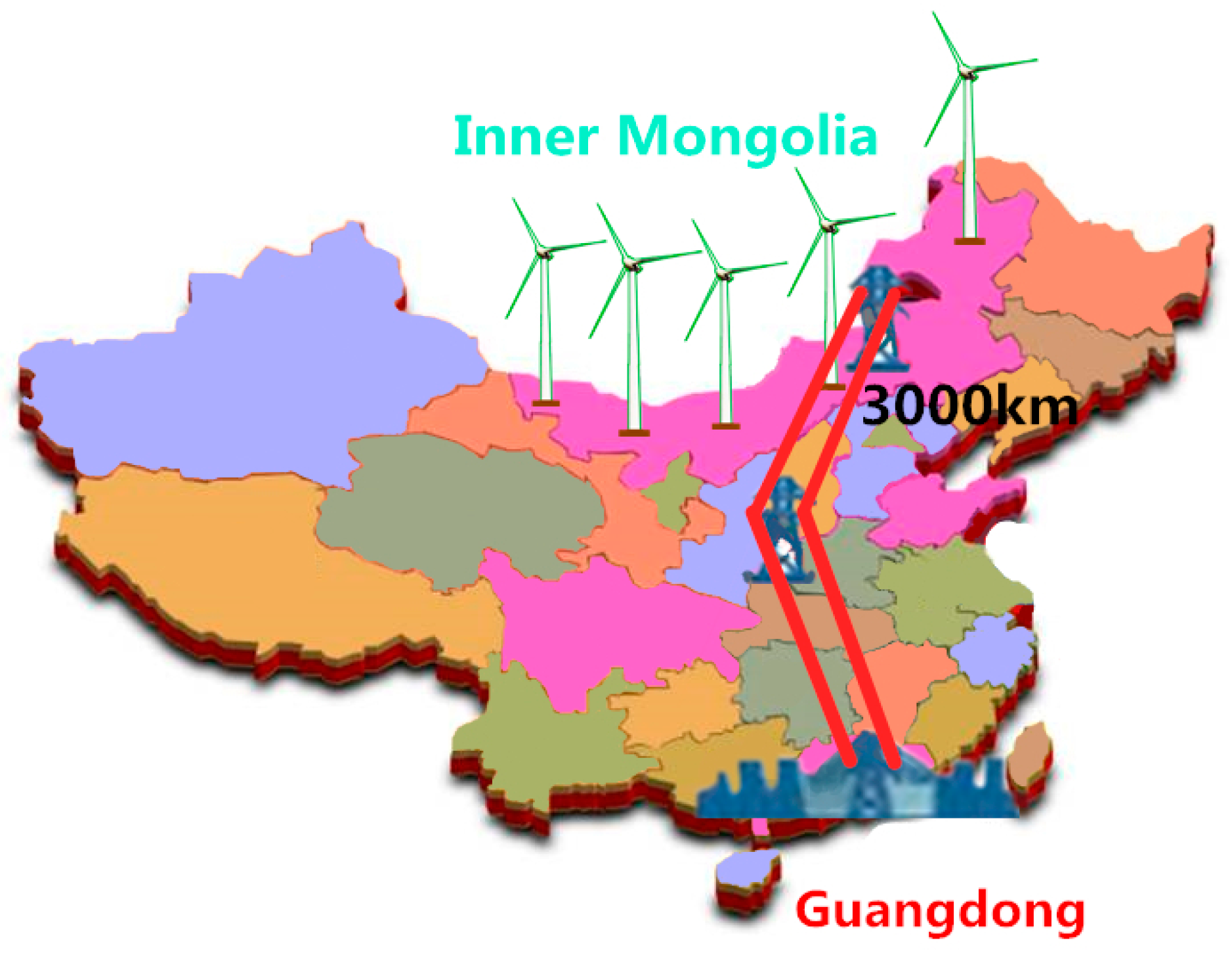The high-voltage direct current (HVDC) transmission system is believed to be a plausible method for bulk power transmission over long distances [11], but the extremely high cost of ultra-high voltage power electronic devices is the main obstacle to wide application of HVDC. Furthermore, the distance between the large-scale wind farms and load centers in China is usually thousands of kilometers [12], thus the half-wavelength transmission line (HWTL) without reactive power compensation or intermediate substations has been considered as a promising alternative for long-distance transmission of bulk renewable energy [13].

Although the concept of natural half-wavelength power transmission has been proposed since 1939 [14], the overvoltage, power demands, and other technical problems in modern power systems are very different from the past. Due to the constant fundamental frequency of 50 Hz or 60 Hz, the length of HWTL is fixed at about 3000 km or 2500 km [15], which restricts its practical application. Consequently, a compensation algorithm was proposed in [16] to transform a transmission line shorter than half-wavelength to the tuned HWTL with lumped compensation circuit by inductance and capacitance. In addition, ref. [17] analyzed the differences in overvoltage, voltage distribution, and current distribution between tuned HWTL and natural HWTL. In order to reduce the differences between natural HWTL and tuned HWTL, a lumped compensation circuit was divided into a series of sections and the effects of different sections were thoroughly compared in [18]. Moreover, ref. [19] attempted to generate high frequency from 180 Hz to 360 Hz to make half-wavelength lines suitable for short-distance transmission, in which an AC-AC or AC-DC-AC conversion is required to transform high-frequency power to a 50 Hz or 60 Hz component for traditional fundamental frequency loads.

Generally speaking, HWTL can be adversely affected by extreme environmental conditions, e.g., storms [20], lightning [21], forest fires [22], and ice shedding [23]; such conditions can significantly reduce the air gaps between transmission lines or easily exceed the threshold of insulators, so that a breakdown of transmission line insulation might occur. For the purpose of quickly locating the fault point, several fault location algorithms have been proposed and developed over the past decades, which can be generally classified into the following three groups: (a) fundamental frequency–based method [24], (b) transmission line differential equations [25], and (c) travelling wave method [26]. In particular, they are suitable for different fault types and causes. The first one only needs a low-frequency sampling rate (around 6.4 kHz) but a long time window of voltage and current (>20 ms) [27]; the second one requires accurate transmission line impedance and a high-frequency sampling rate (around 10 kHz) of voltage and current [25]; the third one requires an ultra-high-frequency sampling rate (>500 kHz) and a short time window (<5 ms) of current or voltage, in which the signal magnitude will be inevitably decayed in HWTL [28].

In fact, the above three approaches are all based on the following two techniques: (1) single-end data–based fault location [29] and (2) double-end data–based fault location [30]. Normally, the fault location accuracy of the former can be considerably degraded as the distance of transmission line increases. Although the fault location accuracy of the latter is insensitive to transmission line distance, it requires accurate synchronous voltages and currents of double ends, which are hard to obtain in HWTL. To handle this challenge, this paper proposes a modal voltage distribution–based asynchronous double-end fault location (MVD-ADFL) method that does not require synchronous voltages and currents. It merely needs a low-frequency sampling rate (around 6.4 kHz) and a long time window of voltage and current (around 20 ms). At first, the modal voltages and currents are calculated from three asynchronous phases by applying phase-modal transformation matrix. Then, the voltages distributed along the modal circuit are calculated from double ends independently. Finally, the fault point is chosen from the interconnection points of modal voltages distributed along transmission lines or the minimum of particular air modal voltage distributions along transmission lines.

The rest of this paper is organized as follows: Section 2 is devoted to modelling of parallel multiconductor transmission lines, and Section 3 develops the wavelength calculations of different modes in HWTL. Section 4 presents the design of the MVD-ADFL method for HWTL. In Section 5, simulation and real-time digital simulator (RTDS)–based hardware-in-the-loop (HIL) test results on different fault types, distances, resistances, and wind generator capacities are presented to verify the effectiveness of MVD-ADFL. Section 6 presents a discussion of the adaptivity of MVD-ADFL and the influence of generator types. Finally, some conclusions and possible future studies are summarized in Section 7.

2. Modelling of Parallel Multiconductor Transmission Lines

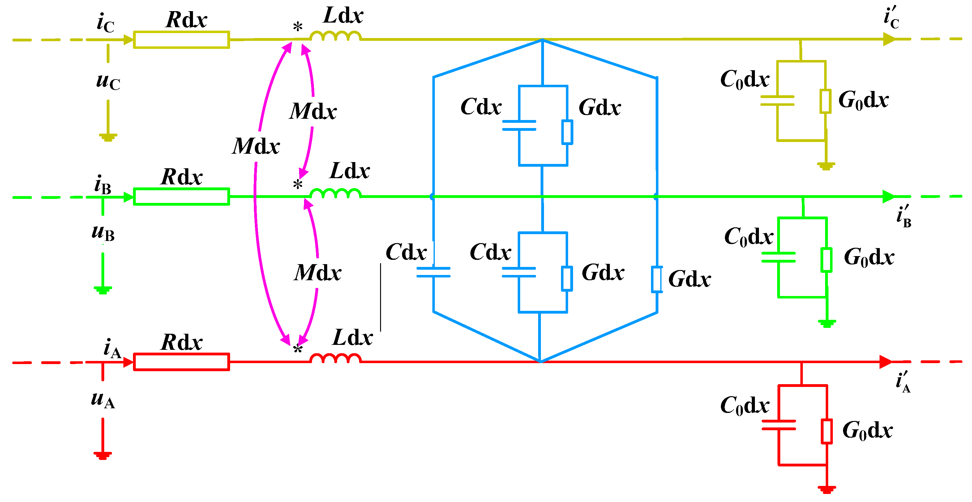
Three-phase transmission lines can be approximated by aggregating equivalent circuit segments distributed along the lines. A line segment with length dx can be represented by an equivalent resistor, inductor and capacitor (RLC) circuit, as illustrated in Figure 1, in which the parameters of three lines are assumed to be identical in this paper.

The equations of lossy three-phase transmission lines with constant parameters can be written as

$$\{\begin{array}{c}-\frac{\partial i_{\mathrm{A}}}{\partial x}=(G_0+2G)u_{\mathrm{A}}+(C_0+2C)\frac{\partial u_{\mathrm{A}}}{\partial t}-G(u_{\mathrm{B}}+u_{\mathrm{C}})-C(\frac{\partial u_{\mathrm{B}}}{\partial t}+\frac{\partial u_{\mathrm{C}}}{\partial t})\\ -\frac{\partial i_{\mathrm{B}}}{\partial x}=(G_0+2G)u_{\mathrm{B}}+(C_0+2C)\frac{\partial u_{\mathrm{B}}}{\partial t}-G(u_{\mathrm{A}}+u_{\mathrm{C}})-C(\frac{\partial u_{\mathrm{A}}}{\partial t}+\frac{\partial u_{\mathrm{C}}}{\partial t})\\ -\frac{\partial i_{\mathrm{C}}}{\partial x}=(G_0+2G)u_{\mathrm{C}}+(C_0+2C)\frac{\partial u_{\mathrm{C}}}{\partial t}-G(u_{\mathrm{A}}+u_{\mathrm{B}})-C(\frac{\partial u_{\mathrm{A}}}{\partial t}+\frac{\partial u_{\mathrm{B}}}{\partial t})\end{array},$$

(1)

$$\{\begin{array}{c}-\frac{\partial u_{\mathrm{A}}}{\partial x}=R{i}_{\mathrm{A}}+L\frac{\partial i_{\mathrm{A}}}{\partial t}+M(\frac{\partial i_{\mathrm{B}}}{\partial t}+\frac{\partial i_{\mathrm{C}}}{\partial t})\\ -\frac{\partial u_{\mathrm{B}}}{\partial x}=R{i}_{\mathrm{B}}+L\frac{\partial i_{\mathrm{B}}}{\partial t}+M(\frac{\partial i_{\mathrm{A}}}{\partial t}+\frac{\partial i_{\mathrm{C}}}{\partial t})\\ -\frac{\partial u_{\mathrm{C}}}{\partial x}=R{i}_{\mathrm{C}}+L\frac{\partial i_{\mathrm{C}}}{\partial t}+M(\frac{\partial i_{\mathrm{A}}}{\partial t}+\frac{\partial i_{\mathrm{B}}}{\partial t})\end{array},$$

(2)

where u_μ and i_μ are the voltage and current of phase μ (μ = A, B, and C), respectively; G₀ and C₀ are the conductance and capacitance per unit (p.u.) length between line and earth, respectively; G, C, and M are the conductance, capacitance, and mutual inductance between line and line in p.u., respectively; and R and L are the line resistance and inductance in p.u., respectively.

If only one frequency component needs to be analyzed in voltage and current, the time-domain Equations (1) and (2) can be transformed to the following frequency-domain equation:

$$\{\begin{array}{c}-\frac{\mathrm{d}{\stackrel{⌢}{I}}_{\mathrm{A}}}{\mathrm{d}x}=(G_0+2G){\stackrel{⌢}{U}}_{\mathrm{A}}+j\omega (C_0+2C){\stackrel{⌢}{U}}_{\mathrm{A}}-G({\stackrel{⌢}{U}}_{\mathrm{B}}+{\stackrel{⌢}{U}}_{\mathrm{C}})-j\omega C({\stackrel{⌢}{U}}_{\mathrm{B}}+{\stackrel{⌢}{U}}_{\mathrm{C}})\\ -\frac{\mathrm{d}{\stackrel{⌢}{I}}_{\mathrm{B}}}{\mathrm{d}x}=(G_0+2G){\stackrel{⌢}{U}}_{\mathrm{B}}+j\omega (C_0+2C){\stackrel{⌢}{U}}_{\mathrm{B}}-G({\stackrel{⌢}{U}}_{\mathrm{A}}+{\stackrel{⌢}{U}}_{\mathrm{C}})-j\omega C({\stackrel{⌢}{U}}_{\mathrm{A}}+{\stackrel{⌢}{U}}_{\mathrm{C}})\\ -\frac{\mathrm{d}{\stackrel{⌢}{I}}_{\mathrm{C}}}{\mathrm{d}x}=(G_0+2G){\stackrel{⌢}{U}}_{\mathrm{C}}+j\omega (C_0+2C){\stackrel{⌢}{U}}_{\mathrm{C}}-G({\stackrel{⌢}{U}}_{\mathrm{A}}+{\stackrel{⌢}{U}}_{\mathrm{B}})-j\omega C({\stackrel{⌢}{U}}_{\mathrm{A}}+{\stackrel{⌢}{U}}_{\mathrm{B}})\end{array},$$

(3)

$$\{\begin{array}{c}-\frac{\mathrm{d}{\stackrel{⌢}{U}}_{\mathrm{A}}}{\mathrm{d}x}=R{\stackrel{⌢}{I}}_{\mathrm{A}}+j\omega L{\stackrel{⌢}{I}}_{\mathrm{A}}+j\omega M({\stackrel{⌢}{I}}_{\mathrm{B}}+{\stackrel{⌢}{I}}_{\mathrm{C}})\\ -\frac{\mathrm{d}{\stackrel{⌢}{U}}_{\mathrm{B}}}{\mathrm{d}x}=R{\stackrel{⌢}{I}}_{\mathrm{B}}+j\omega L{\stackrel{⌢}{I}}_{\mathrm{B}}+j\omega M({\stackrel{⌢}{I}}_{\mathrm{A}}+{\stackrel{⌢}{I}}_{\mathrm{C}})\\ -\frac{\mathrm{d}{\stackrel{⌢}{U}}_{\mathrm{C}}}{\mathrm{d}x}=R{\stackrel{⌢}{I}}_{\mathrm{C}}+j\omega L{\stackrel{⌢}{I}}_{\mathrm{C}}+j\omega M({\stackrel{⌢}{I}}_{\mathrm{A}}+{\stackrel{⌢}{I}}_{\mathrm{B}})\end{array},$$

(4)

where the angular frequency ω = 2πf; ${\stackrel{⌢}{U}}_{\mu }$ and ${\stackrel{⌢}{I}}_{\mu }$ are the voltage and current of phase μ in the frequency domain, f is the fundamental frequency, and j is the imaginary unit. Equations (3) and (4) are the three-phase wave equations.

The wave equations can be obtained from Equations (3) and (4) as

$$\{\begin{array}{c}-\frac{{\mathrm{d}}^2{\stackrel{⌢}{U}}_{\mathrm{A}}}{\mathrm{d}{x}^2}=(R+j\omega L)\frac{\mathrm{d}{\stackrel{⌢}{I}}_{\mathrm{A}}}{\mathrm{d}x}+j\omega M(\frac{\mathrm{d}{\stackrel{⌢}{I}}_{\mathrm{B}}}{\mathrm{d}x}+\frac{\mathrm{d}{\stackrel{⌢}{I}}_{\mathrm{C}}}{\mathrm{d}x})\\ -\frac{{\mathrm{d}}^2{\stackrel{⌢}{U}}_{\mathrm{B}}}{\mathrm{d}{x}^2}=(R+j\omega L)\frac{\mathrm{d}{\stackrel{⌢}{I}}_{\mathrm{B}}}{\mathrm{d}x}+j\omega M(\frac{\mathrm{d}{\stackrel{⌢}{I}}_{\mathrm{A}}}{\mathrm{d}x}+\frac{\mathrm{d}{\stackrel{⌢}{I}}_{\mathrm{C}}}{\mathrm{d}x})\\ -\frac{{\mathrm{d}}^2{\stackrel{⌢}{U}}_{\mathrm{C}}}{\mathrm{d}{x}^2}=(R+j\omega L)\frac{\mathrm{d}{\stackrel{⌢}{I}}_{\mathrm{C}}}{\mathrm{d}x}+j\omega M(\frac{\mathrm{d}{\stackrel{⌢}{I}}_{\mathrm{B}}}{\mathrm{d}x}+\frac{\mathrm{d}{\stackrel{⌢}{I}}_{\mathrm{A}}}{\mathrm{d}x})\end{array},$$

(5)

$$\{\begin{array}{c}-\frac{{\mathrm{d}}^2{\stackrel{⌢}{I}}_{\mathrm{A}}}{\mathrm{d}{x}^2}=(G_0+2G+j\omega C_0+2j\omega C)\frac{\mathrm{d}{\stackrel{⌢}{U}}_{\mathrm{A}}}{\mathrm{d}x}+-(G+j\omega C)(\frac{\mathrm{d}{\stackrel{⌢}{U}}_{\mathrm{B}}}{\mathrm{d}x}+\frac{\mathrm{d}{\stackrel{⌢}{U}}_{\mathrm{C}}}{\mathrm{d}x})\\ -\frac{{\mathrm{d}}^2{\stackrel{⌢}{I}}_{\mathrm{B}}}{\mathrm{d}{x}^2}=(G_0+2G+j\omega C_0+2j\omega C)\frac{\mathrm{d}{\stackrel{⌢}{U}}_{\mathrm{B}}}{\mathrm{d}x}+-(G+j\omega C)(\frac{\mathrm{d}{\stackrel{⌢}{U}}_{\mathrm{A}}}{\mathrm{d}x}+\frac{\mathrm{d}{\stackrel{⌢}{U}}_{\mathrm{C}}}{\mathrm{d}x})\\ -\frac{{\mathrm{d}}^2{\stackrel{⌢}{I}}_{\mathrm{C}}}{\mathrm{d}{x}^2}=(G_0+2G+j\omega C_0+2j\omega C)\frac{\mathrm{d}{\stackrel{⌢}{U}}_{\mathrm{C}}}{\mathrm{d}x}+-(G+j\omega C)(\frac{\mathrm{d}{\stackrel{⌢}{U}}_{\mathrm{B}}}{\mathrm{d}x}+\frac{\mathrm{d}{\stackrel{⌢}{U}}_{\mathrm{A}}}{\mathrm{d}x})\end{array},$$

(6)

In order to reduce the complexity of the equation, phase A is taken as an example. The relationship between $\frac{{\mathrm{d}}^2{\stackrel{⌢}{U}}_{\mathrm{A}}}{\mathrm{d}{x}^2}$ and ${\stackrel{⌢}{U}}_{\mathrm{A}}$, $\frac{{\mathrm{d}}^2{\stackrel{⌢}{I}}_{\mathrm{A}}}{\mathrm{d}{x}^2}$ and ${\stackrel{⌢}{I}}_{\mathrm{A}}$ can be written as

$$\begin{array}{lll}\frac{{\mathrm{d}}^2{\stackrel{⌢}{U}}_{\mathrm{A}}}{\mathrm{d}{x}^2}& =& (R+j\omega L)[(G_0+2G+j\omega C_0+2j\omega C){\stackrel{⌢}{U}}_{\mathrm{A}}-(G+j\omega C)({\stackrel{⌢}{U}}_{\mathrm{B}}+{\stackrel{⌢}{U}}_{\mathrm{C}})]\\ & & +j\omega M[(G_0+G+j\omega C_0+j\omega C)({\stackrel{⌢}{U}}_{\mathrm{B}}+{\stackrel{⌢}{U}}_{\mathrm{C}})-2(G+j\omega C){\stackrel{⌢}{U}}_{\mathrm{A}}]\\ & =& \frac{1}{3}[2(R+j\omega L-j\omega M)(G_0+3G+j\omega C_0+3j\omega C){\stackrel{⌢}{U}}_{\mathrm{A}}+(R+j\omega L+2j\omega M)(G_0+j\omega C_0){\stackrel{⌢}{U}}_{\mathrm{A}}\\ & & +(R+j\omega L+2j\omega M)(G_0+j\omega C_0)({\stackrel{⌢}{U}}_{\mathrm{B}}+{\stackrel{⌢}{U}}_{\mathrm{C}})\\ & & -(R+j\omega L-j\omega M)(G_0+3G+j\omega C_0+3j\omega C)({\stackrel{⌢}{U}}_{\mathrm{B}}+{\stackrel{⌢}{U}}_{\mathrm{C}})]\end{array},$$

(7)

$$\begin{array}{lll}\frac{{\mathrm{d}}^2{\stackrel{⌢}{I}}_{\mathrm{A}}}{\mathrm{d}{x}^2}& =& (G_0+2G+j\omega C_0+2j\omega C)[(R+j\omega L){\stackrel{⌢}{I}}_{\mathrm{A}}+j\omega M({\stackrel{⌢}{I}}_{\mathrm{B}}+{\stackrel{⌢}{I}}_{\mathrm{C}})]\\ & & -(G+j\omega C)[(R+j\omega L+j\omega M)({\stackrel{⌢}{I}}_{\mathrm{B}}+{\stackrel{⌢}{I}}_{\mathrm{C}})+2j\omega M{\stackrel{⌢}{I}}_{\mathrm{A}}]\\ & =& \frac{1}{3}[2(R+j\omega L-j\omega M)(G_0+3G+j\omega C_0+3j\omega C){\stackrel{⌢}{I}}_{\mathrm{A}}+(R+j\omega L+2j\omega M)(G_0+j\omega C_0){\stackrel{⌢}{I}}_{\mathrm{A}}\\ & & +(R+j\omega L+2j\omega M)(G_0+j\omega C_0)({\stackrel{⌢}{I}}_{\mathrm{B}}+{\stackrel{⌢}{I}}_{\mathrm{C}})\\ & & -(R+j\omega L-j\omega M)(G_0+3G+j\omega C_0+3j\omega C)({\stackrel{⌢}{I}}_{\mathrm{B}}+{\stackrel{⌢}{I}}_{\mathrm{C}})]\end{array}$$

(8)

Equations (7) and (8) are both ordinary differential equations, thus their solutions can be obtained as

$${\stackrel{⌢}{U}}_{\mathrm{A}}=\frac{2}{3}(A_1{e}^{-{\gamma }_{1}x}+A_2{e}^{{\gamma }_{1}x})+\frac{1}{3}(A_3{e}^{-{\gamma }_{0}x}+A_4{e}^{{\gamma }_{0}x})+\frac{1}{3}(A_5{e}^{-{\gamma }_{1}x}+A_6{e}^{{\gamma }_{1}x})+\frac{1}{3}(A_7{e}^{-{\gamma }_{0}x}+A_8{e}^{{\gamma }_{0}x}),$$

(9)

$${\stackrel{⌢}{I}}_{\mathrm{A}}=\frac{2}{3}(B_1{e}^{-{\gamma }_{1}x}+B_2{e}^{{\gamma }_{1}x})+\frac{1}{3}(B_3{e}^{-{\gamma }_{0}x}+B_4{e}^{{\gamma }_{0}x})+\frac{1}{3}(B_5{e}^{-{\gamma }_{1}x}+B_6{e}^{{\gamma }_{1}x})+\frac{1}{3}(B_7{e}^{-{\gamma }_{0}x}+B_8{e}^{{\gamma }_{0}x}),$$

(10)

where

$${\gamma }_0=\sqrt{(R+j\omega L+2j\omega M)(G_0+j\omega C_0)},$$

(11)

$${\gamma }_1=\sqrt{(R+j\omega L-j\omega M)(3G+G_0+3j\omega C+j\omega C_0)},$$

(12)

A₁ to A₄ and B₁ to B₄ are calculated from phase A, while A₅ to A₈ and B₅ to B₈ are from phases B and C.

The voltage and current of the sending end are denoted as

$$P_s=\left[\begin{array}{c}{U}_s\\ I_s\end{array}\right]=\left[\begin{array}{c}{U}_{\mathrm{As}}\\ U_{\mathrm{Bs}}\\ U_{\mathrm{Cs}}\\ I_{\mathrm{As}}\\ I_{\mathrm{Bs}}\\ I_{\mathrm{Cs}}\end{array}\right],$$

(13)

The voltage and current after propagation along transmission lines with number of x can be written as

$$P_x=T{P}_s,$$

(14)

where

$$P_x=\left[\begin{array}{c}{U}_x\\ I_x\end{array}\right]=\left[\begin{array}{c}{U}_{\mathrm{Ax}}\\ U_{\mathrm{Bx}}\\ U_{\mathrm{Cx}}\\ I_{\mathrm{Ax}}\\ I_{\mathrm{Bx}}\\ I_{\mathrm{Cx}}\end{array}\right],$$

(15)

$$T=\left[\begin{array}{cccccc}\frac{2}{3}{H}_1+\frac{1}{3}{H}_2& -\frac{1}{3}{H}_1+\frac{1}{3}{H}_2& -\frac{1}{3}{H}_1+\frac{1}{3}{H}_2& -\frac{2Z_{\mathrm{C}0}}{3}{H}_3-\frac{Z_{\mathrm{C}1}}{3}{H}_4& \frac{Z_{\mathrm{C}0}}{3}{H}_3-\frac{Z_{\mathrm{C}1}}{3}{H}_4& \frac{Z_{\mathrm{C}0}}{3}{H}_3-\frac{Z_{\mathrm{C}1}}{3}{H}_4\\ -\frac{1}{3}{H}_1+\frac{1}{3}{H}_2& \frac{2}{3}{H}_1+\frac{1}{3}{H}_2& -\frac{1}{3}{H}_1+\frac{1}{3}{H}_2& \frac{Z_{\mathrm{C}0}}{3}{H}_3-\frac{Z_{\mathrm{C}1}}{3}{H}_4& -\frac{2Z_{\mathrm{C}0}}{3}{H}_3-\frac{Z_{\mathrm{C}1}}{3}{H}_4& \frac{Z_{\mathrm{C}0}}{3}{H}_3-\frac{Z_{\mathrm{C}1}}{3}{H}_4\\ -\frac{1}{3}{H}_1+\frac{1}{3}{H}_2& -\frac{1}{3}{H}_1+\frac{1}{3}{H}_2& \frac{2}{3}{H}_1+\frac{1}{3}{H}_2& \frac{Z_{\mathrm{C}0}}{3}{H}_3-\frac{Z_{\mathrm{C}1}}{3}{H}_4& \frac{Z_{\mathrm{C}0}}{3}{H}_3-\frac{Z_{\mathrm{C}1}}{3}{H}_4& -\frac{2Z_{\mathrm{C}0}}{3}{H}_3-\frac{Z_{\mathrm{C}1}}{3}{H}_4\\ -\frac{2}{3Z_{\mathrm{C}0}}{H}_3-\frac{1}{3Z_{\mathrm{C}1}}{H}_4& \frac{1}{3Z_{\mathrm{C}1}}{H}_3-\frac{1}{3Z_{\mathrm{C}2}}{H}_4& \frac{1}{3Z_{\mathrm{C}1}}{H}_3-\frac{1}{3Z_{\mathrm{C}2}}{H}_4& \frac{2}{3}{H}_1+\frac{1}{3}{H}_2& -\frac{1}{3}{H}_1+\frac{1}{3}{H}_2& -\frac{1}{3}{H}_1+\frac{1}{3}{H}_2\\ \frac{1}{3Z_{\mathrm{C}1}}{H}_3-\frac{1}{3Z_{\mathrm{C}2}}{H}_4& -\frac{2}{3Z_{\mathrm{C}0}}{H}_3-\frac{1}{3Z_{\mathrm{C}1}}{H}_4& \frac{1}{3Z_{\mathrm{C}1}}{H}_3-\frac{1}{3Z_{\mathrm{C}2}}{H}_4& -\frac{1}{3}{H}_1+\frac{1}{3}{H}_2& \frac{2}{3}{H}_1+\frac{1}{3}{H}_2& -\frac{1}{3}{H}_1+\frac{1}{3}{H}_2\\ \frac{1}{3Z_{\mathrm{C}1}}{H}_3-\frac{1}{3Z_{\mathrm{C}2}}{H}_4& \frac{1}{3Z_{\mathrm{C}1}}{H}_3-\frac{1}{3Z_{\mathrm{C}2}}{H}_4& -\frac{2}{3Z_{\mathrm{C}0}}{H}_3-\frac{1}{3Z_{\mathrm{C}1}}{H}_4& -\frac{1}{3}{H}_1+\frac{1}{3}{H}_2& -\frac{1}{3}{H}_1+\frac{1}{3}{H}_2& \frac{2}{3}{H}_1+\frac{1}{3}{H}_2\end{array}\right],$$

(16)

$$H_1=\cosh ({\gamma }_{0}x),$$

(17)

$$H_2=\cosh ({\gamma }_{1}x),$$

(18)

$$H_3=\sinh ({\gamma }_{0}x),$$

(19)

$$H_4=\sinh ({\gamma }_{1}x),$$

(20)

where ${\gamma }_0$ and ${\gamma }_1$ are the propagation constants and $Z_{\mathrm{C}0}$ and $Z_{\mathrm{C}1}$ are characteristic impedances, as follows:

$$Z_{\mathrm{C}0}=\sqrt{\frac{R+j\omega L+2j\omega M}{G_0+j\omega C_0}},$$

(21)

$$Z_{\mathrm{C}1}(s)=\sqrt{\frac{R+j\omega L-j\omega M}{3G+G_0+3j\omega C+j\omega C_0}},$$

(22)

As shown in Equations (6)–(22), the voltage and current propagated along any transmission line will be affected by electromagnetic waves travelling along other parallel conductors due to the coupling of electromagnetic fields. If the characteristics of multiconductor transmission lines are symmetric, the electromagnetic wave propagating along those lines can be represented by the sum of three-phase voltage and current, with two different propagation constants and two different characteristic impedances. In order to simplify the analysis of travelling waves in multiconductor transmission lines, the impedance matrix and admittance matrix are transformed to diagonal matrices, of which each diagonal element denotes the impedance and admittance of an uncoupled circuit, and the phase voltage and phase current are transformed to modal voltage and modal current that propagate along the special uncoupled circuit. In particular, most of the uncoupled circuits, e.g., air mode, represent the circuit between conductors, while one of them is the circuit named “earth mode” between line and earth.

3. Wavelength Calculation of Different Modes in HWTL

3.1. Configuration of HWTL in China

The largest onshore wind farm in the world is located in Gangsu and Inner Mongolia in northern China, while the load centers are concentrated in southeast coastal areas thousands of kilometers away from. As a result, large amounts of electricity generated by the wind farm cannot be effectively transmitted to the load centers, which wastes a huge amount of wind power annually. On the other hand, the coastal load centers frequently encounter load-peak shifting in summer due to power shortages. In order to solve the dilemma of wasted wind power and power shortages in different areas, bulk power transmission technology over long distances becomes a crucial task.

The 1000 kV alternating current (AC) transmission line was implemented and has been operating as a demonstration project for ultra-high-voltage extra-long-distance transmission in China since 2009. The large-scale wind farms in northern China are nearly 3000 km away from load centers in Guangdong, as schematically shown in Figure 2, which makes half-wavelength transmission geographically possible.

3.2. Wavelength Calculation of Ultra-High-Voltage HWTL

Due to the long distance, the half-wavelength transmission line needs a high-voltage level to reduce energy loss. Thus most research on half-wavelength is based on ultra-high-voltage, such as 1000 kV or higher. In this paper, the 1000 kV tower implemented in Jingdongnan-Nanyang-Jingmen is studied as demonstrated in Figure 3.

The air modal propagation constant γ₁ and earth modal propagation constant γ₀ become

$${\gamma }_1={\alpha }_1+j{\beta }_1=\sqrt{(R_1+j\omega L_1)j\omega C_1},$$

(23)

$${\gamma }_0={\alpha }_0+j{\beta }_0=\sqrt{(R_0+j\omega L_0)j\omega C_0},$$

(24)

where R₁, L₁, and C₁ are the air modal resistance, inductance, and capacitance, respectively, and R₀, L₀, and C₀ are earth modal resistance, inductance, and capacitance, respectively. Wavelength is a variable that changes with the imaginary part of the propagation constant, therefore the air modal wavelength at fundamental frequency λ₁ and the earth modal wavelength at fundamental frequency λ₀ are written as

$${\lambda }_1=\frac{2\pi }{{\beta }_1}=\frac{2\pi }{\sqrt{\frac{1}{2}{\omega }^2{L}_1{C}_1+\sqrt{{\omega }^2{C}_1^2(R_1^2+{\omega }^2{L}_1^2)}}},$$

(25)

$${\lambda }_0=\frac{2\pi }{{\beta }_0}=\frac{2\pi }{\sqrt{\frac{1}{2}{\omega }^2{L}_0{C}_0+\sqrt{{\omega }^2{C}_0^2(R_0^2+{\omega }^2{L}_0^2)}}},$$

(26)

It can be seen from Equations (25) and (26) that the air modal wavelength will be different from the earth modal wavelength. Although the phase voltage distribution satisfies the air modal half-wavelength distribution in normal operation due to the balanced three phases, the asymmetric parameters, unbalanced operation, or asymmetric fault may distort the voltage distribution along transmission lines.

If the multiconductor transmission lines are ideally transposed, the characteristic impedances of all air modes are identical. However, the characteristic impedance of earth mode usually varies greatly with frequency, due to its propagation channel between lines and ground, thus earth modal impedance is much different from air modal impedance. More specifically, if the transmission line is short, the voltage distribution along that line and the different modal characteristics have no significant influence on line protection or overvoltage, but the half-wavelength line is too long to ignore the influence of different wavelength of modes.

4. Modal Voltage Distribution–Based Asynchronous Double-End Fault Location

4.1. Phase-Modal Transformation

Considering the different characteristics of air mode and earth mode, the phase current and voltage can be transformed into modal components by the Karenbauer transform matrix [31] as

$$\left[\begin{array}{c}{\stackrel{⌢}{U}}_{\alpha }\\ {\stackrel{⌢}{U}}_{\beta }\\ {\stackrel{⌢}{U}}_{\chi }\\ {\stackrel{⌢}{U}}_0\end{array}\right]=\left[\begin{array}{ccc}1& -1& 0\\ 1& 0& -1\\ 0& 1& -1\\ 1& 1& 1\end{array}\right]\left[\begin{array}{c}{\stackrel{⌢}{U}}_A\\ {\stackrel{⌢}{U}}_B\\ {\stackrel{⌢}{U}}_C\end{array}\right],$$

(27)

A two-port network is used to represent the ideally transposed line by

$$\left[\begin{array}{c}{\stackrel{⌢}{U}}_{\phi x}\\ {\stackrel{⌢}{I}}_{\phi x}\end{array}\right]=\left[\begin{array}{cc}\cosh ({\gamma }_{\phi }x)& -Z_{c\phi }\sinh ({\gamma }_{\phi }x)\\ -\frac{1}{Z_{c\phi }}\sinh ({\gamma }_{\phi }x)& \cosh ({\gamma }_{\phi }x)\end{array}\right]\left[\begin{array}{c}{\stackrel{⌢}{U}}_{\phi s}\\ {\stackrel{⌢}{I}}_{\phi s}\end{array}\right],$$

(28)

where φ = 0, α, β and χ. U_φs and I_φs are the sending end voltage and current, respectively; U_φx and I_φx are voltage and current away from sending end with distance x, respectively; γ_α, γ_β, and γ_χ are all equal to γ₁; and Z_cα, Z_cβ, and Z_cχ are all equal to Z_c1. The modes α, β, and χ are all air modes with different circuits, while their characteristics are almost the same if the transmission lines are ideally transposed. On the other hand, the voltage distributed along transmission lines can also be obtained by the voltage and current of the receiving end, as follows:

$$\left[\begin{array}{c}{\stackrel{⌢}{U}}_{\phi lx}\\ {\stackrel{⌢}{I}}_{\phi lx}\end{array}\right]=\left[\begin{array}{cc}\cosh ({\gamma }_{\phi }(l-x))& Z_{c\phi }\sinh ({\gamma }_{\phi }(l-x))\\ \frac{1}{Z_{c\phi }}\sinh ({\gamma }_{\phi }(l-x))& \cosh ({\gamma }_{\phi }(l-x))\end{array}\right]\left[\begin{array}{c}{\stackrel{⌢}{U}}_{\phi r}\\ {\stackrel{⌢}{I}}_{\phi r}\end{array}\right],$$

(29)

where U_φlr and I_φlr represent the voltage and current of receiving end, respectively, and l is the total length of faulty line. Here, each point in the ideally transposed line has the same voltage, calculated by Equations (28) and (29), but the fault point is a boundary of ideally transposed line, which makes the real voltage different from the calculated voltage. Since the transform matrix cannot decouple the fault point resulting from the three-phase unbalance at the fault point, the actual voltage and the calculated voltage are quite different in the region between the fault point and the remote end.

4.2. Fault Location of Phase-to-Ground Fault

The fault point separates the line into two sections, in which the actual voltage is similar to the calculated voltage at the near end but much different at the remote end. Hence, the calculated voltage from each end may obtain the same value at fault point but much different values at other points. The fault distance can be written as

$$x=\frac{1}{{\gamma }_{\varphi }}{\tanh }^{-1}\left[\frac{Z_{c\varphi }{\stackrel{⌢}{I}}_{r\varphi }\sinh ({\gamma }_{\varphi }l)-{\stackrel{⌢}{U}}_{r\varphi }\cosh ({\gamma }_{\varphi }l)+{\stackrel{⌢}{U}}_{s\varphi }}{Z_{c\varphi }{\stackrel{⌢}{I}}_{r\varphi }\cosh ({\gamma }_{\varphi }l)-{\stackrel{⌢}{U}}_{r\varphi }\sinh ({\gamma }_{\varphi }l)+Z_{c\varphi }{\stackrel{⌢}{I}}_{s\varphi }}\right],$$

(30)

where x could be a complex number with a small imaginary part due to the numerical calculation error, thus the fault distance can be written as

$$x=\left|\frac{1}{{\gamma }_{\varphi }}{\tanh }^{-1}\left[\frac{Z_{c\varphi }{\stackrel{⌢}{I}}_{r\varphi }\sinh ({\gamma }_{\varphi }l)-{\stackrel{⌢}{U}}_{r\varphi }\cosh ({\gamma }_{\varphi }l)+{\stackrel{⌢}{U}}_{s\varphi }}{Z_{c\varphi }{\stackrel{⌢}{I}}_{r\varphi }\cosh ({\gamma }_{\varphi }l)-{\stackrel{⌢}{U}}_{r\varphi }\sinh ({\gamma }_{\varphi }l)+Z_{c\varphi }{\stackrel{⌢}{I}}_{s\varphi }}\right]\right|,$$

(31)

where l is the line length. Equation (31) needs synchronized measurements from both ends. However, numerous factors, such as thunderstorms and electromagnetic interference, will degrade the synchronization accuracy. The fault location method with unsynchronized data from both ends shall be discussed.

The angle of fundamental frequency voltage and current are time-varying, but their amplitude is stable when the fault transients are attenuated. Considering the voltage amplitude, Equation (30) can be rewritten as

$$\begin{array}{l}\left|Z_{c\varphi }{\stackrel{⌢}{I}}_{r\varphi }\sinh ({\gamma }_{\varphi }l)\cosh ({\gamma }_{\varphi }x)-{\stackrel{⌢}{U}}_{r\varphi }\cosh ({\gamma }_{\varphi }l)\cosh ({\gamma }_{\varphi }x)+{\stackrel{⌢}{U}}_{s\varphi }\cosh ({\gamma }_{\varphi }x)\right|\\ =\left|Z_{c\varphi }{\stackrel{⌢}{I}}_{r\varphi }\cosh ({\gamma }_{\varphi }l)\sinh ({\gamma }_{\varphi }x)-{\stackrel{⌢}{U}}_{r\varphi }\sinh ({\gamma }_{\varphi }l)\sinh ({\gamma }_{\varphi }x)+Z_{c\varphi }{\stackrel{⌢}{I}}_{s\varphi }\sinh ({\gamma }_{\varphi }x)\right|\end{array},$$

(32)

If the transmission lines are ideally transposed, the characteristic impedances of all air modes are almost the same. Thus, only the air modal circuit containing the faulty phase line is selected to calculate the voltage distribution. Thus, Equation (32) becomes

$$\begin{array}{l}\left|Z_{c1}{\stackrel{⌢}{I}}_{r1}\sinh ({\gamma }_{1}l)\cosh ({\gamma }_{1}x)-{\stackrel{⌢}{U}}_{r1}\cosh ({\gamma }_{1}l)\cosh ({\gamma }_{1}x)+{\stackrel{⌢}{U}}_{s1}\cosh ({\gamma }_{1}x)\right|\\ =\left|Z_{c1}{\stackrel{⌢}{I}}_{r1}\cosh ({\gamma }_{1}l)\sinh ({\gamma }_{1}x)-{\stackrel{⌢}{U}}_{r1}\sinh ({\gamma }_{1}l)\sinh ({\gamma }_{1}x)+Z_{c1}{\stackrel{⌢}{I}}_{s1}\sinh ({\gamma }_{1}x)\right|\end{array},$$

(33a)

$$\begin{array}{l}\left|Z_{c0}{\stackrel{⌢}{I}}_{r0}\sinh ({\gamma }_{0}l)\cosh ({\gamma }_{0}x)-{\stackrel{⌢}{U}}_{r0}\cosh ({\gamma }_{0}l)\cosh ({\gamma }_{0}x)+{\stackrel{⌢}{U}}_{s0}\cosh ({\gamma }_{0}x)\right|\\ =\left|Z_{c0}{\stackrel{⌢}{I}}_{r0}\cosh ({\gamma }_{0}l)\sinh ({\gamma }_{0}x)-{\stackrel{⌢}{U}}_{r0}\sinh ({\gamma }_{0}l)\sinh ({\gamma }_{0}x)+Z_{c0}{\stackrel{⌢}{I}}_{s0}\sinh ({\gamma }_{0}x)\right|\end{array},$$

(33b)

Here, the calculated voltage distribution along transmission lines between the fault point and the remote end are quite different from the real voltage distribution. However, it may obtain intersection points with calculated voltage from another end casually. As a result, Equations (33a) and (33b) might contain multiple solutions, while additional conditions should be taken into account to accomplish an accurate fault location. Moreover, Equations (33a) and (33b) always have the similar fault location estimation near the fault point, and the characteristics of different modes lead to different periods of voltage distribution along transmission lines, so inaccurate fault location estimations can be eliminated by the significant difference between the air mode and earth estimations. Denoting the air mode fault location estimation as x₁ and the earth mode fault location estimation as x₀, the following inequality needs to be satisfied:

$$|x_1-x_0|\le \eta ,$$

(34)

where η is the threshold between x₁ and x₀, and η is set as 5% × 3000 km = 150 km in this paper.

The calculation error and non-ideal models may lead to some differences between fault location estimation of air mode and earth mode, while their mean value is used for an accurate fault location result x_f1 as

$$x_{\mathrm{f}1}=\frac{x_1+x_0}{2}$$

(35)

4.3. Fault Location of Phase-to-Phase Fault

If the transmission line fault is a phase-to-phase fault, where the fault point is still insulated to ground, the earth modal voltage will equal zero. Hence, a fault location scheme without zero modal voltage has to be considered.

The modal voltage transformed by the phase-modal transformation matrix in Equation (27) can be regarded as the voltage in an independent two-conductor modal circuit formed by two phase lines. If two faulty phase lines are applied to form the air modal circuit, the voltage of the fault point will be the minimum. Therefore, the minimum of the calculated voltage along transmission lines can be calculated from double ends to locate the fault point of phase-to-phase fault. The fault location can be represented as

$${\stackrel{⌢}{U}}_{\min r}(x_r)=\min \left|Z_{c1}{\stackrel{⌢}{I}}_{r1}\sinh ({\gamma }_{1}l)\cosh ({\gamma }_{1}x)-{\stackrel{⌢}{U}}_{r1}\cosh ({\gamma }_{1}l)\cosh ({\gamma }_{1}x)\right|,$$

(36a)

$${\stackrel{⌢}{U}}_{\min s}(x_s)=\min \left|Z_{c1}{\stackrel{⌢}{I}}_{s1}\sinh ({\gamma }_{1}l)\cosh ({\gamma }_{1}x)-{\stackrel{⌢}{U}}_{s1}\cosh ({\gamma }_{1}l)\cosh ({\gamma }_{1}x)\right|,$$

(36b)

Ideally, the minimum voltage distribution along transmission lines calculated by Equations (36a) and (36b) from double ends should be similar, and the next local minimum should be one-half air modal wavelength away, such that the fault point can be treated as the global minimum in almost all faults. In addition, the calculation error increases as the distance grows, hence most of the fault location is more reliable in dealing with near-end fault. The calculated distance of the fault point can be used as the weight ω_r for receiving-end fault location estimation x_r, and weight ω_s for sending-end fault location estimation x_s, which gives fault location result x_f2 as

$$x_{\mathrm{f}2}={\omega }_r{x}_r+{\omega }_s{x}_s,$$

(37)

where

$$\{\begin{array}{c}{\omega }_r=\frac{x_r}{l}\\ {\omega }_s=\frac{l-x_s}{l}\end{array},$$

(38)

4.4. Overall Fault Location Scheme

If the methods in Section 4.2 and Section 4.3 are applied for a fault, the final fault location result x_f can be written as

$$x_{\mathrm{f}}=\frac{x_{\mathrm{f}1}+x_{\mathrm{f}2}}{2},$$

(39)

To this end, the overall fault location scheme can be summarized in the following three procedures:

(1)

Determine the faulty phase and fault type by reference [13] with a low-frequency sampling rate.

(2)

Apply transform matrix to obtain modal voltage and modal current, and choose an appropriate modal circuit containing double faulty phases for voltage distribution calculation and fault location.

(3)

If the fault type includes a ground fault, apply the intersection points of different modal voltage distributions to locate the fault distance. Otherwise, the fault distance will be located by both intersection points and minimum.

The overall flowchart of MVD-ADFL is demonstrated in Figure 4.

5. Case Studies

5.1. Simulation Model

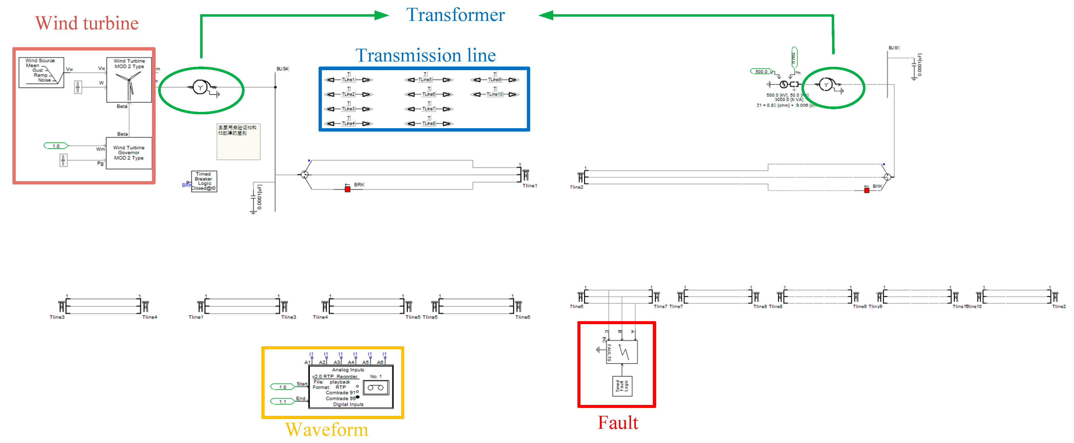
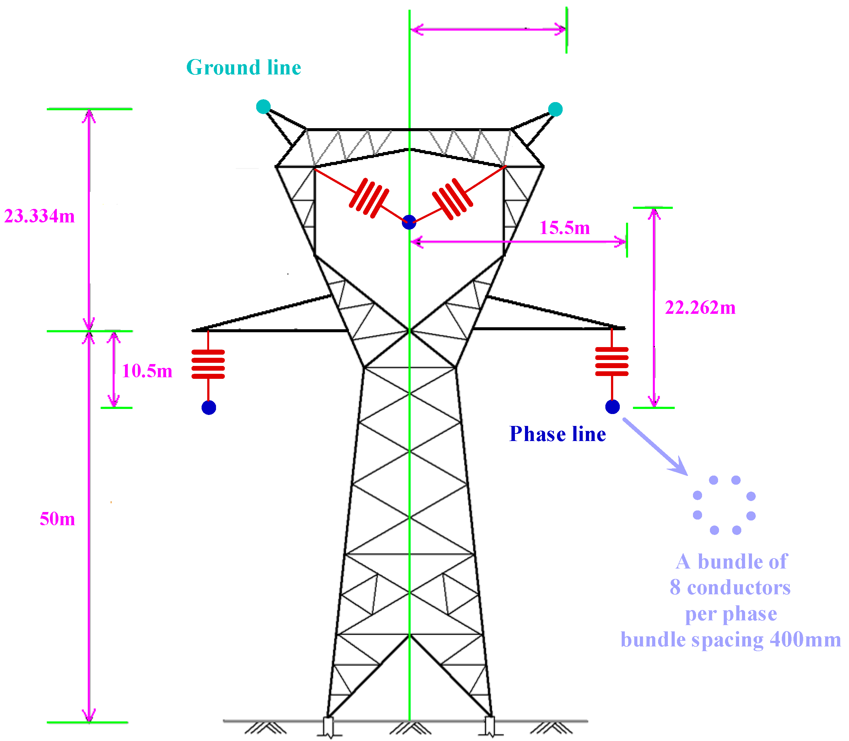
A schematic diagram of the simulation model is depicted in Figure 5, while the tower shown in Figure 3 is used to calculate the transmission line parameters. Two hundred doubly fed induction generators [32] with 3 MW rated power and 25 m/s rated wind speed were considered for the wind farm, and were aggregated into an equivalent 600 MW generator in the model. The tower shown in Figure 3 was used to calculate the transmission line parameters. Bus M and bus N represent the sending and receiving end of transmission lines, respectively.

Power Systems Computer Aided Design/Electromagnetic Transients including DC (PSCAD/EMTDC), an electromagnetic time-domain transient simulation environment created by Manitoba Hydro International with a library of preprogrammed models and a design editor for building custom models to satisfy various levels of different modelling demands, was adopted to construct a simulation model of HWTL with large-scale wind power integration; version 4.5 was used in this study [33,34,35,36,37]. The simulation tests were implemented based on the PSCAD/EMTDC model, a general-purpose time-domain simulation tool for studying transient behavior of electrical networks. A single line diagram of the simulation model is provided in Figure 6, and its parameters are given in

Table 1. Parameters of the transformer at bus M.

Transformer MVA	1000.0 MVA
Base Operation Frequency	50 Hz
Leakage Reactance	0.1 p.u.
High-Voltage (HV) Winding Voltage	1100 kV
Low-Voltage (LV) Winding Voltage	500 kV

,

Table 2. Parameters of the transformer at bus N.

Transformer MVA	1000.0 MVA
Base Operation Frequency	50 Hz
Leakage Reactance	0.1 p.u.
HV Winding Voltage	1000 kV
LV Winding Voltage	550 kV

and

Table 3. Parameters of the wind turbine.

Generator Rate MVA	3 MVA
Rated Wind Speed	12 m/s
Air Density	1.225 kg/m3
Resistance of Stator Winding	0.005 p.u.
Resistance of Rotator Winding	0.0055 p.u.
Leakage Inductance of Stator Winding	0.4 p.u.
Leakage Inductance of Stator Winding	0.44 p.u.

.

The frequency-dependent model was employed to represent transmission lines in the simulation.

Table 4. Parameters of different modes.

Mode	Resistance (Ω/m)	Inductance (H/m)	Capacitance (F/m)	Wavelength (m)
Air mode	R1 = 1.032 × 10−5	L1 = 8.404 × 10−7	C1 = 1.375 × 10−11	λ1 = 5.882 × 106
Earth mode	R0 = 2.513 × 10−4	L0 = 2.692 × 10−6	C0 = 8.804 × 10−12	λ0 = 4.065 × 106

shows the frequency-dependent parameters of transmission line when the fundamental frequency is 50 Hz, based on the tower shown in Figure 3 [38].

It can be seen in Table 4 that the air mode wavelength is much larger than earth mode due to the differences between air modal circuit and earth modal circuit, hence the open-phase operation and unbalanced ground fault can induce quite different voltage distributions in air modal circuit and earth modal circuit.

Normally, wind farms are required to achieve maximum power point tracking to track the optimal active power curve, which is obtained by connecting each maximum power point at various wind speeds with the optimal active power curve determined by

$$P_{\mathrm{opt}}({\omega }_{\mathrm{m}})=K^{*}{\omega }_{\mathrm{m}}^3,$$

(40)

where $K^{*}=0.5\rho \pi R^5{C}_{\mathrm{P}}^{*}/{({\lambda }^{*})}^3$ denotes the shape coefficient of optimal active power, R is the blade radius of the wind turbine, ρ is the air density, the optimal tip-speed ratio ${\lambda }^{*}=7.4$, and the maximum power coefficient $C_{\mathrm{P}}^{*}=0.4019$ [33].

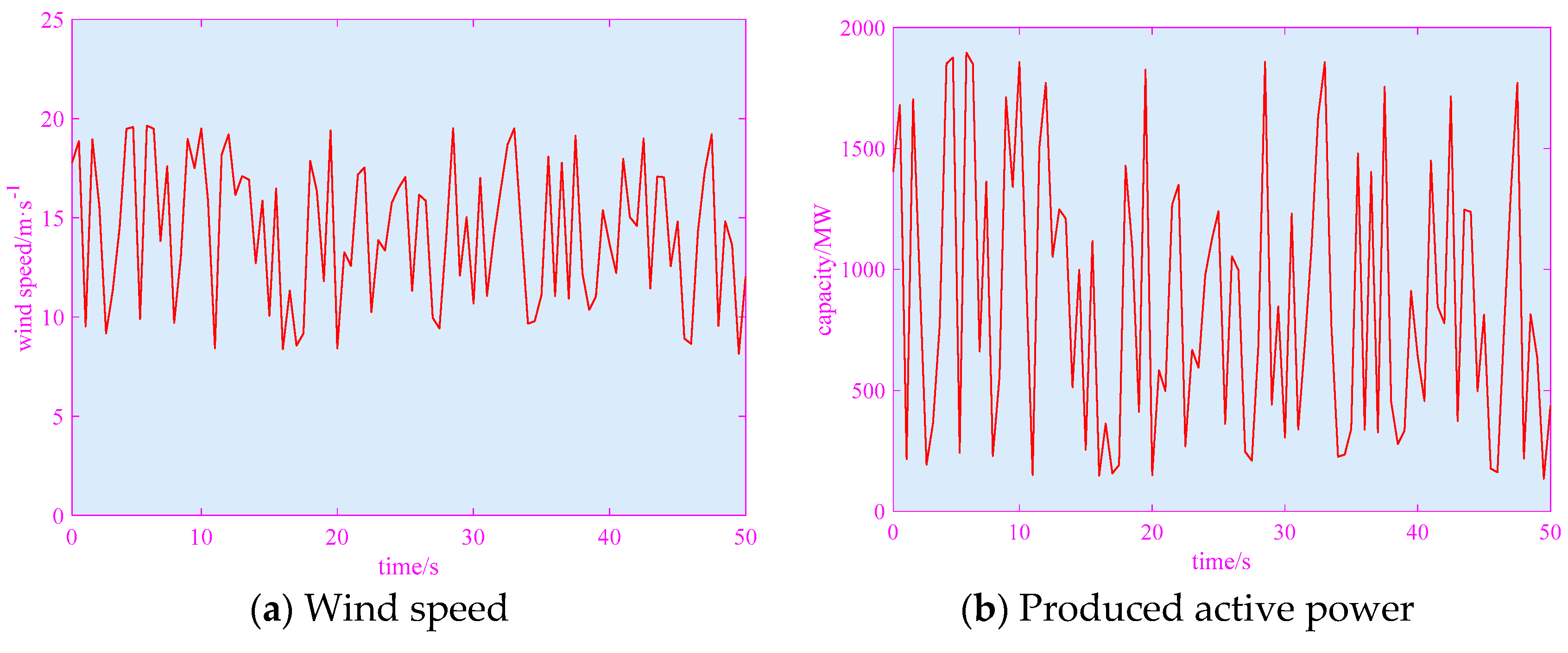
Hence, the power generated from the wind farm usually has a highly stochastic pattern, which will be injected into the main power grid [31]. Figure 7a,b demonstrate the wind speed and produced active power of the wind farm, respectively.

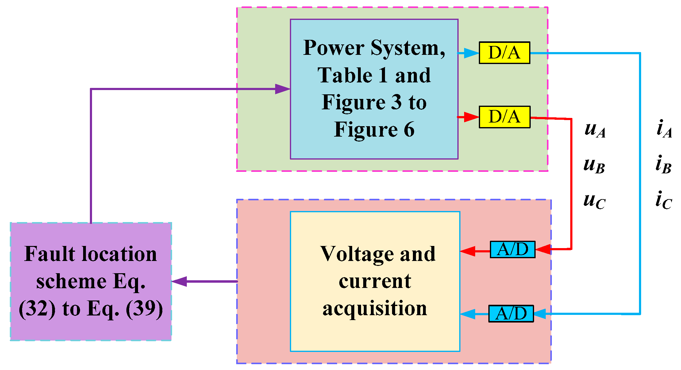
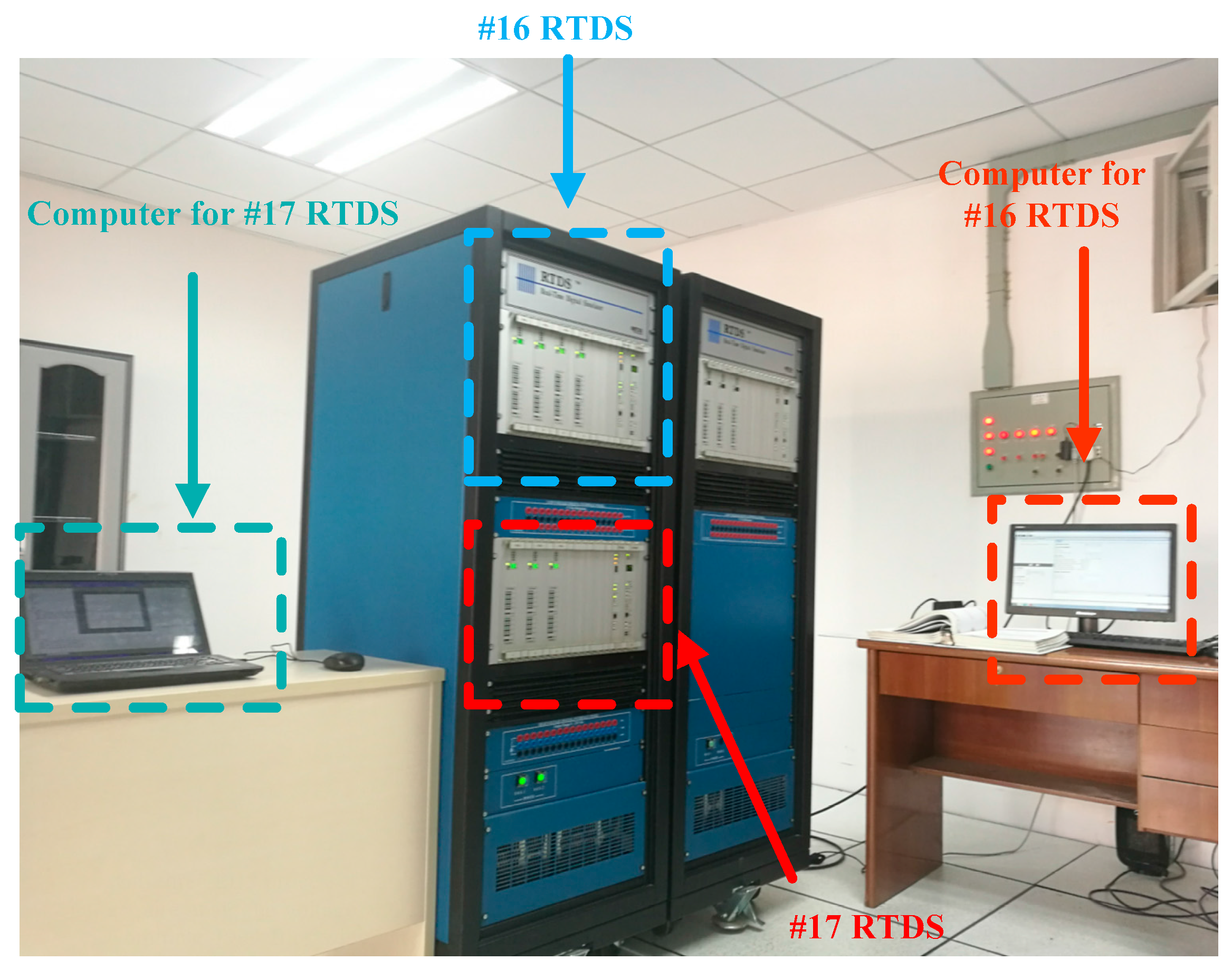
The hardware-in-the-loop (HIL) test is a powerful and important technique that has been used worldwide in real-time experiments instead of practical experiments due to the complexity and large scale of real power systems. The Real-Time Digital Simulator (RTDS), which is capable of closed-loop testing of protection and control equipment, was adopted in this study to further validate the feasibility of hardware implementation. The configuration and experimental platform of HIL test are provided in Figure 8 and Figure 9.

A power system with a sampling rate of 20 kHz was implemented by #16 RTDS with four PB5 processor cards and one gigabit transceiver analog output card, which can output the voltage and current at bus M and bus N. Meanwhile, #17 RTDS with three PB5 processor cards and one gigabit transceiver analog input card was applied as an acquisition device with 10 kHz to acquire voltage and current output from #16 RTDS. The voltage and current acquired by #17 RTDS was transferred to digital data and stored in RTDS as Common format for Transient Data Exchange (COMTRADE) 1999 files, which were then transmitted to a PC with an IntelR Core™ i3 CPU at 2.52 GHz and 3 GB of RAM. Finally, the voltage and current waveforms were decoded from COMTRADE 1999 files in the PC to locate fault points by the proposed MVD-ADFL.

Denoting the fault distance as x_fault, the relative fault location calculation error ε is defined as

$$\epsilon =\frac{|x_{\mathrm{f}}-x_{\mathrm{fault}}|}{l}\times 100\%,$$

(41)

where l is the total length of fault line and x_f is the fault location result.

5.2. Single Phase-to-Ground Fault

A phase-to-ground (AG) fault with 200 Ω fault resistance, 2400 km away from bus M, which occurred at 10 s with a total wind power of 180 MW, was investigated by simulation and HIL test. The calculated voltage distribution along transmission lines from bus M and bus N are shown in Figure 10.

There are two intersection points calculated by air mode and three intersection points calculated by earth mode voltage distribution in the PSCAD simulation and the HIL test, as shown in Figure 10. In the PSCAD simulation, 2365 km and 2249 km in air mode and 2365 km in earth mode satisfy Equation (34), thus the fault location result is

$$\frac{\frac{2365\mathrm{km}+2249\mathrm{km}}{2}+2365\mathrm{km}}{2}=2326\mathrm{km}$$

In the HIL test, only 2425 km in air mode and 2374 km in earth mode satisfy Equation (34), and the fault location result is

$$\frac{2425\mathrm{km}+2374\mathrm{km}}{2}=2390\mathrm{km}$$

The fault location results of simulation and HIL tests are tabulated in

Table 5. Fault location estimation of AG fault.

Test	Fault Location Result (km)	ε (%)
Simulation	2326	2.46
HIL	2390	0.33

.

It can be clearly seen that the voltage distribution along transmission lines of HIL is almost the same as the that of the simulation, therefore the fault location results of the simulation and the HIL test are similar. The errors of fault location results based on the simulation and the HIL test are 2.46% and 0.33%, respectively.

5.3. Phase-to-Phase Fault

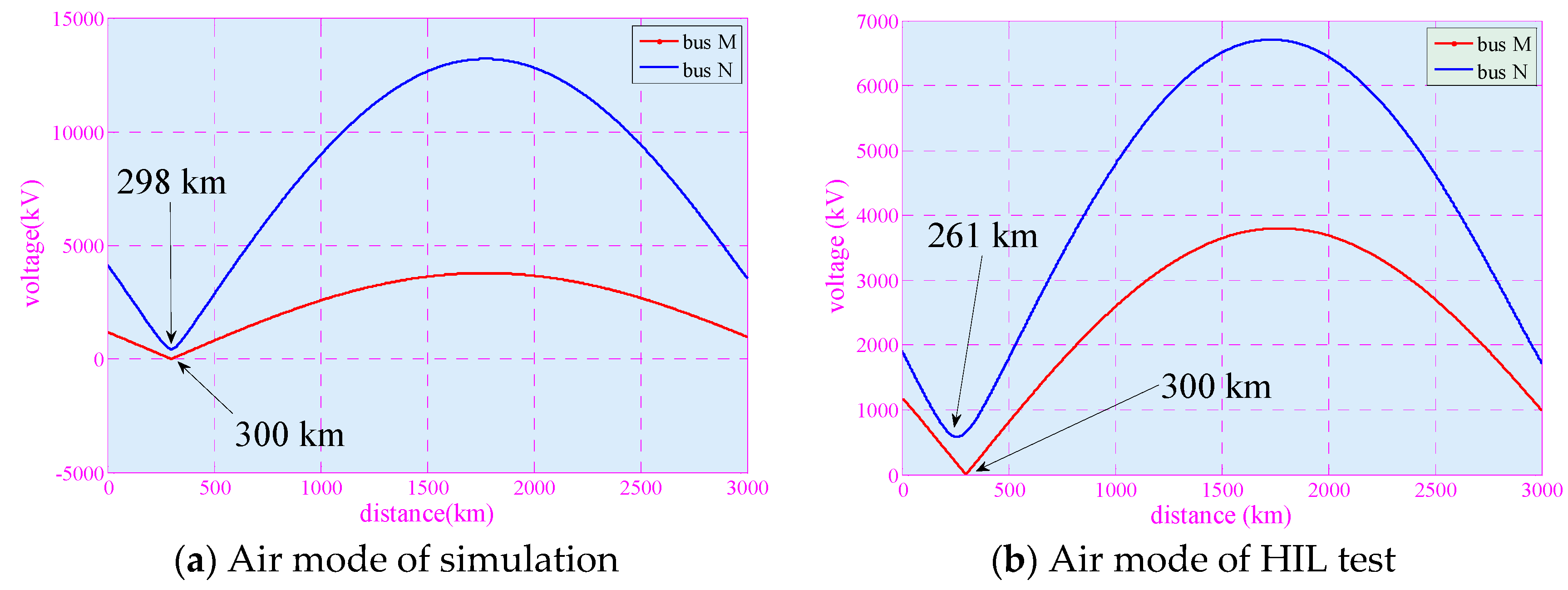
A phase-A-to-phase-B (AB) fault with 10 Ω fault resistance, 300 km away from bus M, which occurred with 210 MW wind power at 20 s, was investigated. The calculated voltage distributions along transmission lines from bus M and bus N are given in Figure 11.

The AB fault point is nearly ideal, thus the minimums of air modal and earth modal voltage distribution along transmission lines are similar. In the PSCAD simulation, 300 km and 298 km are the minimum in air mode, hence the fault location result is

$$298\mathrm{km}\times \frac{298}{3000}+300\mathrm{km}\times \frac{3000-300}{3000}=300\mathrm{km}$$

In the HIL test, 261 km and 300 km are the minimum in air mode, and the fault location result is

$$261\mathrm{km}\times \frac{261}{3000}+300\mathrm{km}\times \frac{3000-300}{3000}=294\mathrm{km}$$

Table 6. AB fault location results of simulation and HIL test.

Test	Fault Location Result (km)	ε (%)
Simulation	300	0.00
HIL	294	0.20

demonstrates the fault location results of the simulation and the HIL tests.

The AB fault point is a nearly ideal boundary for the air mode circuit containing phase A and phase B, thus the minimums of air modal and earth modal voltage distribution along transmission lines are similar. The fault location error of the simulation is 0.00 and of the HIL test is 0.20. Even though the error of the HIL test is larger than that of the simulation, it is acceptable.

5.4. Double Phase-to-Ground Fault

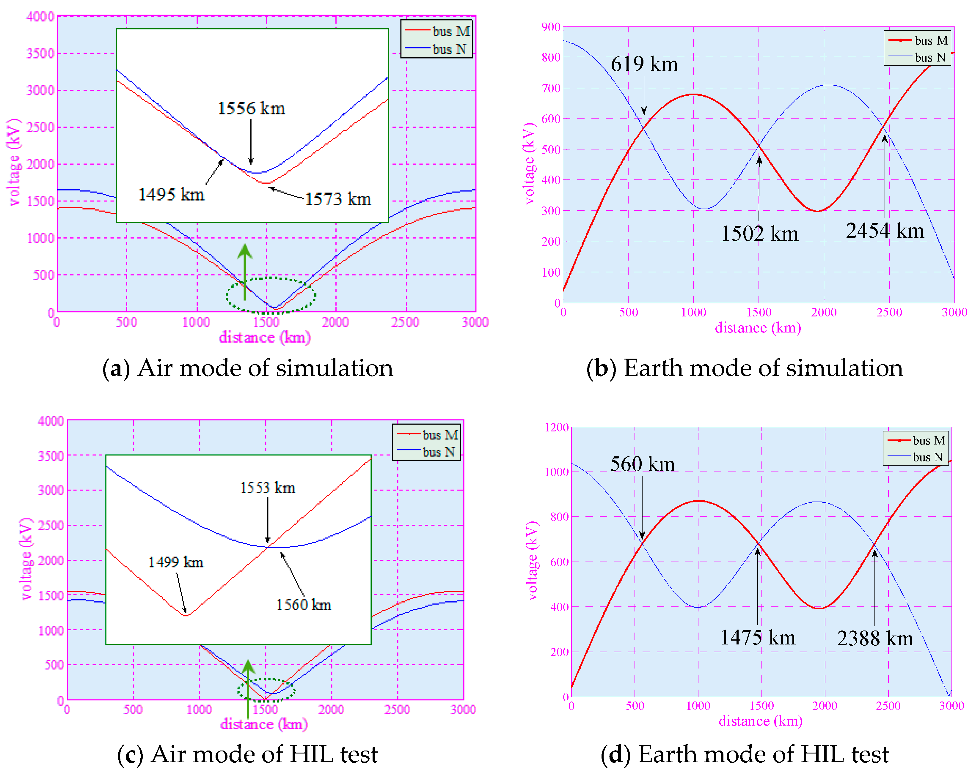
A double phase-to-ground (ABG) fault with 50 Ω fault resistance, 1500 km away from bus M was studied, while fault occurred at 30 s with 400 MW produced wind power. The calculated voltage distributions along transmission lines from bus M and bus N are presented in Figure 12.

Here, both the intersection points and minimum method can be applied for fault location estimation of ABG fault. In the PSCAD simulation, the intersection point in air mode, 1495 km, and minimums, 1556 km and 1573 km, are all close to 1502 km, one of the intersection points in earth mode voltage distribution, therefore the fault location result is

$$\frac{1495\mathrm{km}+1556\mathrm{km}\times \frac{1556}{3000}+1573\mathrm{km}\times \frac{3000-1573}{3000}}{2}=1552\mathrm{km}$$

In the HIL test, the intersection point in air mode is 1553 km and the minimums are 1499 km and 1560 km. The fault location result is

$$\frac{1553\mathrm{km}+1560\mathrm{km}\times \frac{1560}{3000}+1499\mathrm{km}\times \frac{3000-1499}{3000}}{2}=1551\mathrm{km}$$

The fault location results of the simulation and the HIL tests are illustrated in

Table 7. Location results of ABG fault.

Test	Fault Location Result (km)	ε (%)
Simulation	1552	1.76
HIL	1551	1.76

.

Here, both the intersection points and minimum method can be applied for fault location estimation. Lastly, the fault location results of the simulation and the HIL test are almost the same, and fault location errors are both 1.76%.

5.5. Three-Phase Fault

A three-phase (ABC) fault with 10 Ω fault resistance, 1800 km away from bus M, was simulated at 50 s, with 550 MW produced wind power. The calculated voltage distribution along transmission lines from bus M and bus N are illustrated in Figure 13, and the fault location estimations are provided in

Table 8. Location estimation of ABC fault.

Test	Fault Location Result (km)	ε (%)
Simulation	1799	0.03
HIL	1765	1.17

.

Only minimums of voltage distributions are applied in this case, but all the minimums are close to the fault point. In the PSCAD simulation, the minimums are 1788 km and 1809 km, so the fault location result is obtained as

$$1809\mathrm{km}\times \frac{1809}{3000}+1788\mathrm{km}\times \frac{3000-1788}{3000}=1799\mathrm{km}$$

In the HIL test, the minimums are 1741 km and 1799 km, and the fault location result is

$$1741\mathrm{km}\times \frac{1741}{3000}+1799\mathrm{km}\times \frac{3000-1799}{3000}=1765\mathrm{km}$$

The fault location results of the simulation and the HIL test can be found in Table 8.

The minimums of air voltage distributions are similar in the simulation and the HIL test, so the minimums are applied to estimate the fault location. The fault location error of the simulation is just 0.03%, which is smaller than that of the HIL test; however, the fault location error of the HIL test is just 1.17% and acceptable in the practical implementation.

Comprehensive simulations and HIL tests in the presence of different fault distances, resistances, types, and wind power penetration were carried out to fully verify the effectiveness of MVD-ADFL, which are only summarized in

Table 9. Fault location results of simulation and HIL test.

Fault Distance (km)	100	200	500	450	650	720	830	1020	1675	1740	2200	2900
Produced Wind Power (MW)	120	500	180	300	550	280	600	400	140	570	450	350
Fault Type	AG	AB	ABC	ABG	AG	ABC	ABG	AB	ABC	AG	AB	AG
Fault Resistance (Ω)	200	0	100	50	20	30	10	20	10	80	20	100
Fault Location Result of Simulation (km)	114	201	531	463	618	721	877	1012	1699	1711	2184	2868
ε of Simulation (%)	0.50	0.03	1.03	0.43	1.07	2.30	1.57	0.27	0.8	0.97	0.53	1.07
Fault Location Result of HIL Test (km)	111	213	527	469	615	725	868	1034	1681	1770	2177	2851
ε of HIL Test (%)	0.37	0.43	0.90	0.63	1.17	0.17	1.27	0.47	0.13	1.00	0.77	1.67

due to page limits.

Due to the ideal boundary formed by at least two conductors in the case of air mode of AB and ABC, the MVD-ADFL fault location results of AB and ABC faults are better than those of AG and ABG faults. Additionally, HIL tests and PSCAD simulation are based on different electromagnetic transient program engines, thus some fault location results of HIL tests are even better than those of the PSCAD simulation. Considering the inevitable high-frequency noise in the data acquisition of HIL tests, the good performance of MVD-ADFL in HIL tests indicates that the proposed fault location method is not sensitive enough to the high-frequency noise in the voltage and current waveforms.

6. Discussion

6.1. Adaptability of MVD-ADFL for Any Long Transmission Lines

AC transmission lines cannot be any longer due to the cost of compensation increasing rapidly with line distance, thus traditional AC transmission lines between two substations are dozens to hundreds of kilometers, which is much shorter than the half-wavelength of power system frequency. As a result, there will generally be only one intersection point in either air mode or earth mode voltage distribution if the fault location method based on voltage distribution is applied in traditional transmission lines, as shown in [1]. Furthermore, the different intersection points of earth mode and air mode are utilized to identify the right fault location results in HWTL fault location, but this identification process is unnecessary due to there being only one intersection point in each mode.

6.2. Generator Type

The wind turbine was selected in this paper because the integration of large-scale wind power is a prominent issue for further development of wind energy in China. Electricity transmission from northern China to the load centers in the coastal region is quite inefficient, and the local electricity consumption capability is extremely insufficient due to extreme weather and geographical conditions. Therefore, half-wavelength transmission lines are proposed for bulk wind power transmission, and the wind generator was chosen as the background for our half-wavelength transmission line fault location study. Additionally, due to the wide implementation of doubly fed induction generators in large-scale wind farms, these are applied as the wind turbine type in this study.

The proposed MVD-ADFL method is based on the angle and magnitude of the fundamental frequency voltage and current, which vary with the power generated by wind turbines. The generated power depends on wind speed, which is unstable and unpredictable in most cases. The frequent variation of electrical power, which is rare in solar, hydro, and fossil fuel power generation processes, can be seen as a disturbance to the stable frequency component and an unfavorable factor in the fundamental frequency–based fault location method, therefore wind turbines can reduce the accuracy of the proposed method.

7. Conclusions

In this paper, an MVD-ADFL was developed for HWTL with large-scale wind power integration. The main contributions of this paper can be summarized into the following four aspects:

(1)

The proposed MVD-ADFL is based on transmission line parameters and voltage and current at fundamental frequency. Therefore, traditional low-frequency voltage and current measurement devices are applicable to MVD-ADFL, which offers wide implementation in practice.

(2)

The application of voltage amplitude avoids the accurate synchronization of double-end voltage and current. If synchronous voltage and current are available, they can be used to further reduce calculation errors in fault location.

(3)

Simulation results of different case studies have verified that MVD-ADFL is quite effective for different fault types, while it is insensitive to fault distance, fault resistance, and stochastic wind power variation.

(4)

The RTDS-based HIL test validates the feasibility of implementing MVD-ADFL in different cases.

Future study will investigate the asymmetrical characteristics of non-ideally transposed line to improve the fault location performance of MVD-ADFL in a more practical scenario.

References

1. Yang, B.; Sang, Y.Y.; Shi, K.; Yao, W.; Jiang, L.; Yu, T. Design and real-time implementation of perturbation observer based sliding-mode control for VSC-HVDC systems. Control Eng. Pract. 2016, 56, 13–26. [Google Scholar] [CrossRef]
2. Han, Y.; Xu, C.; Xu, G.; Zhang, Y.W.; Yang, Y.P. An improved flexible solar thermal energy integration process for enhancing the coal-based energy efficiency and NOx removal effectiveness in coal-fired power plants under different load conditions. Energies 2017, 10, 1485. [Google Scholar] [CrossRef]
3. Hooman, K.; Huang, X.X.; Jiang, F.M. Solar-enhanced air-cooled heat exchangers for geothermal power plants. Energies 2017, 10, 1676. [Google Scholar] [CrossRef]
4. Maheshwari, Z.; Ramakumar, R. Smart integrated renewable energy systems (SIRES): A novel approach for sustainable development. Energies 2017, 10, 1145. [Google Scholar] [CrossRef]
5. Ligus, M. Evaluation of economic, social and environmental effects of low-emission energy technologies development in Poland: A multi-criteria analysis with application of a fuzzy analytic hierarchy process. Energies 2017, 10, 1550. [Google Scholar] [CrossRef]
6. Yao, W.; Jiang, L.; Wen, J.Y.; Wu, Q.H.; Cheng, S.J. Wide-area damping controller for power system inter-area oscillations: A networked predictive control approach. IEEE Trans. Control Syst. Technol. 2015, 23, 27–36. [Google Scholar] [CrossRef]
7. Yang, B.; Yu, T.; Shu, H.C.; Zhang, Y.M.; Chen, J.; Sang, Y.Y.; Jiang, L. Passivity-based sliding-mode control design for optimal power extraction of a PMSG based variable speed wind turbine. Renew. Energy 2018, 119, 577–589. [Google Scholar] [CrossRef]
8. Chinese Electric Almanac Committee. Chinese Electric Almanac in 2016; China Electric Power Press: Beijing, China, 2017; pp. 526–528. (In Chinese) [Google Scholar]
9. Yang, B.; Jiang, L.; Wang, L.; Yao, W.; Wu, Q.H. Nonlinear maximum power point tracking control and modal analysis of DFIG based wind turbine. Int. J. Electr. Power Energy Syst. 2016, 74, 429–436. [Google Scholar] [CrossRef]
10. Yang, B.; Yu, T.; Su, H.; Jiang, L. Robust sliding-mode control of wind energy conversion systems for optimal power extraction via nonlinear perturbation observers. Appl. Energy 2018, 210, 711–723. [Google Scholar] [CrossRef]
11. Santos, M.L.; Jardini, J.A.; Casolari, R.P.; Vasquez-Arnez, R.L.; Saiki, G.Y.; Sousa, T.; Nicola, G.L.C. Power transmission over long distances: Economic comparison between HVDC and half-wavelength line. IEEE Trans. Power Deliv. 2017, 29, 502–509. [Google Scholar] [CrossRef]
12. Yang, B.; Zhang, X.S.; Yu, T.; Shu, H.C.; Fang, Z.H. Grouped grey wolf optimizer for maximum power point tracking of doubly-fed induction generator based wind turbine. Energy Convers. Manag. 2017, 133, 427–443. [Google Scholar] [CrossRef]
13. Fabián, R.G.; Tavares, M.C. Faulted phase selection for half-wavelength power transmission lines. IEEE Trans. Power Deliv. 2017. [Google Scholar] [CrossRef]
14. Silva, E.; Moreira, F.; Tavares, M. Energization simulations of a half-wavelength transmission line when subject to three-phase faults—Application to a field test situation. Electr. Power Syst. Res. 2016, 138, 58–65. [Google Scholar] [CrossRef]
15. Mauricio, A.; Robson, D. FACTS for Tapping and Power Flow Control in Half-Wavelength Transmission Lines. IEEE Trans. Ind. Electron. 2012, 59, 3669–3679. [Google Scholar]
16. Prabhakara, F.S.; Parthasarathy, K.; Rao, H.N.R. Performance of tuned half-wave-length power transmission lines. IEEE Trans. Power Appar. Syst. 2007, PAS-88, 1795–1802. [Google Scholar] [CrossRef]
17. Zhao, Y.X.; Wang, S.F.; Wang, H.X.; Wang, J.; Chen, A.Y.; Xue, T.S. Study on the resettlement modes of half-wavelength tuned network of transmission lines. Electr. Power 2017, 50, 147–152. (In Chinese) [Google Scholar]
18. Jiao, C.; Qi, L.; Cui, X. Compensation technology for electrical length of half-wavelength AC power transmission lines. Power Syst. Technol. 2011, 142, 467–470. (In Chinese) [Google Scholar]
19. Wang, Y.; Xu, W.; Li, Y.W.; Hao, T. High-frequency, half-wavelength power transmission scheme. IEEE Trans. Power Deliv. 2017, 32, 279–284. [Google Scholar] [CrossRef]
20. Zhang, Z.J.; You, J.W.; Zhao, J.Y.; Cheng, Y.; Jiang, X.L.; Li, Y.F. Contamination characteristics of disc-suspension insulator of transmission line in wind tunnel. IET Gener. Transm. Distrib. 2017, 11, 1453–1460. [Google Scholar] [CrossRef]
21. Liu, Z.; Liang, K.; Mezentsev, A.; Enno, S.; Sugier, J.; Füllekrug, M. Variable phase propagation velocity for long-range lightning location system. Radio Sci. 2016, 51, 1806–1815. [Google Scholar] [CrossRef]
22. Li, P.; Huang, D.C.; Ruan, J.J.; Wei, H.; Qin, Z.H.; Long, M.Y.; Pu, Z.H.; Wu, T. Influence of forest fire particles on the breakdown characteristics of air gap. IEEE Trans. Dielectr. Electr. Insul. 2016, 23, 1974–1984. [Google Scholar] [CrossRef]
23. Rui, X.M.; Ji, K.P.; Li, L.; McClure, G. Dynamic response of overhead transmission lines with eccentric ice deposits following shock loads. IEEE Trans. Power Deliv. 2017, 32, 1287–1294. [Google Scholar] [CrossRef]
24. Izykowski, J.; Rosolowski, E.; Balcerek, P.; Fulczyk, M.; Saha, M.M. Accurate noniterative fault location algorithm utilizing two end unsynchronized measurements. IEEE Trans. Power Deliv. 2010, 26, 547–555. [Google Scholar] [CrossRef]
25. Wang, L.; Suonan, J. A fast algorithm to estimate phasor in power systems. IEEE Trans. Power Deliv. 2017, 32, 1147–1156. [Google Scholar] [CrossRef]
26. Danilo, P.; Christo, E.S.; Almeida, R. Location of faults in power transmission lines using the ARIMA method. Energies 2017, 10, 1596. [Google Scholar]
27. Serrano, J.; Platero, C.; López-Toledo, M.; Granizo, R. A new method of ground fault location in 2 × 25 kV railway power supply systems. Energies 2017, 10, 340. [Google Scholar] [CrossRef]
28. Bhatti, A.A. Fault location in active distribution networks using non-synchronized measurements. Int. J. Electr. Power Energy Syst. 2017, 93, 451–458. [Google Scholar]
29. Swaroop, G.; Ashok, P. An Accurate Fault Location Method for Multi-Circuit Series Compensated Transmission Lines. IEEE Trans. Power Syst. 2017, 32, 572–580. [Google Scholar]
30. Zhao, P.; Chen, Q.; Sun, K.; Xi, C.A. Current frequency component-based fault-location method for voltage-source converter-based high-voltage direct current (VSC-HVDC) cables using the s transform. Energies 2017, 10, 115. [Google Scholar] [CrossRef]
31. Saha, M. Fault Location on Power; Springer Press: London, UK, 2009; pp. 52–54. [Google Scholar]
32. Yang, B.; Hu, Y.L.; Huang, H.Y.; Shu, H.C.; Yu, T.; Jiang, L. Perturbation estimation based robust state feedback control for grid connected DFIG wind energy conversion system. Int. J. Hydrogen Energy 2017, 42, 20994–21005. [Google Scholar] [CrossRef]
33. Shen, Y.; Yao, W.; Wen, J.Y.; He, H.B. Adaptive wide-area power oscillation damper design for photovoltaic plant considering delay compensation. IET Gener. Transm. Distrib. 2017. [Google Scholar] [CrossRef]
34. Liao, S.W.; Yao, W.; Han, X.N.; Wen, J.Y.; Cheng, S.J. Chronological operation simulation framework for regional power system under high penetration of renewable energy using meteorological data. Appl. Energy 2017, 203, 816–828. [Google Scholar] [CrossRef]
35. Liu, J.; Wen, J.Y.; Yao, W.; Long, Y. Solution to short-term frequency response of wind farms by using energy storage systems. IET Renew. Power Gener. 2016, 10, 669–678. [Google Scholar] [CrossRef]
36. Yang, B.; Yu, T.; Zhang, X.S.; Huang, L.N.; Shu, H.C.; Jiang, L. Interactive teaching-learning optimizer for parameter tuning of VSC-HVDC systems with offshore wind farm integration. IET Gener. Transm. Distrib. 2018, 12, 678–687. [Google Scholar] [CrossRef]
37. Yang, B.; Yu, T.; Shu, H.C.; Zhang, X.S.; Qu, K.P.; Jiang, L. Democratic joint operations algorithm for optimal power extraction of PMSG based wind energy conversion system. Energy Convers. Manag. 2018, 159, 312–326. [Google Scholar] [CrossRef]
38. Liu, Z. Overvoltage and Insulation of Ultra-High Voltage AC Transmission Lines; China Electric Power Press: Beijing, China, 2014; p. 49. (In Chinese) [Google Scholar]
Figure 1. Equivalent RLC-based transmission line segment.
Energies 11 00593 g001
Figure 2. Geographical location of large-scale wind farm and load centers of China.
Energies 11 00593 g002
Figure 3. A 1000 kV transmission tower.
Energies 11 00593 g003
Figure 4. Overall flowchart of the modal voltage distribution based asynchronous double-end fault location (MVD-ADFL) method.
Energies 11 00593 g004
Figure 5. Schematic diagram of the simulation model.
Energies 11 00593 g005
Figure 6. Single line diagram of the simulation model in PSCAD.
Energies 11 00593 g006
Figure 7. Wind speed and produced active power of the wind farm.
Energies 11 00593 g007
Figure 8. Configuration of the hardware-in-the-loop (HIL) test.
Energies 11 00593 g008
Figure 9. Experimental platform of the HIL test.
Energies 11 00593 g009
Figure 10. A phase-to-ground (AG) fault with 200 Ω fault resistance, 2400 km away from bus M, with 1800 MW wind power.
Energies 11 00593 g010
Figure 11. A phase-A-to-phase-B (AB) fault with 10 Ω fault resistance, 300 km away from bus M, with 210 MW wind power.
Energies 11 00593 g011
Figure 12. A double phase-to-ground (ABG) fault with 50 Ω fault resistance, 1500 km away from bus M, with 400 MW wind power.
Energies 11 00593 g012
Figure 13. A three-phase (ABC) fault with 10 Ω fault resistance, 1800 km away from bus M, with 550 MW wind power.
Energies 11 00593 g013