Novel Method for Rapidly Constructing Active Power Steady-State Security Regions Incorporating the Equivalent Reactances of TCSCs

Abstract
:1. Introduction
2. Applicability Analysis of the Existing APSSR Construction Method for a Power System with TCSC
2.1. Brief Illustrations of the Existing APSSR Construction Method
- (1)
- The resistance of transmission lines is much smaller than the reactance, thus Gij ≈ 0. Gij is the element of the real part of the nodal admittance matrix.
- (2)
- Voltage phase angle difference θij of branch i-j is very small, therefore sinθij ≈ θij, cosθij ≈ 1.
2.2. Applicability Analysis for Power System with TCSC
- (1)
- When using Equations (1)–(4) to construct an APSSR of power grid with a TCSC, inversion of the n-order parameter matrix B(XTCSC) is needed.
- (2)
- Moreover, the inversion of a parameter matrix is much more time-consuming than the inversion of a numerical matrix with the same dimension.
3. Derivations of APSSRs with a Single TCSC and Double TCSCs
- (1)
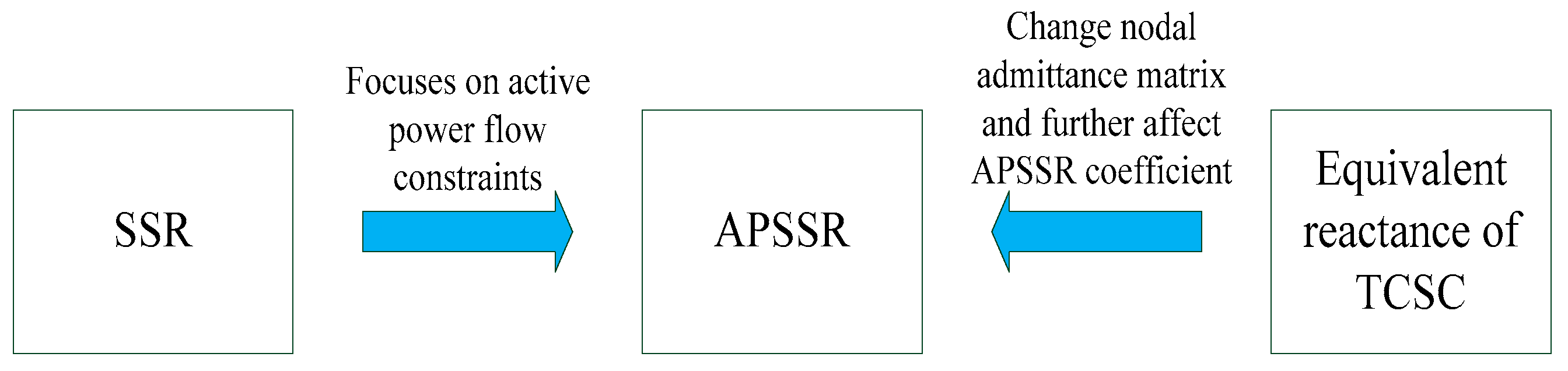
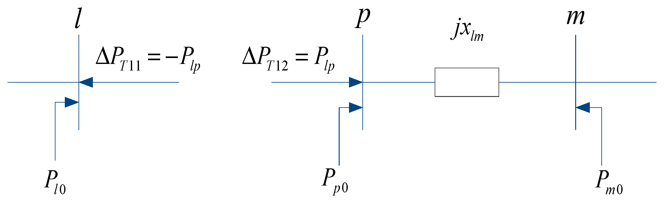
- Via the equivalent disconnection of the TCSC branch, the network structure parameter no longer contains the variable XTCSC, and Y and B will be constant matrices. That is, X = B−1 is also the constant matrix, which can be obtained conveniently.
- (2)
- The effect of XTCSC on the APSSR can be analyzed by influencing node active power injections rather than parameterization of X = B−1.
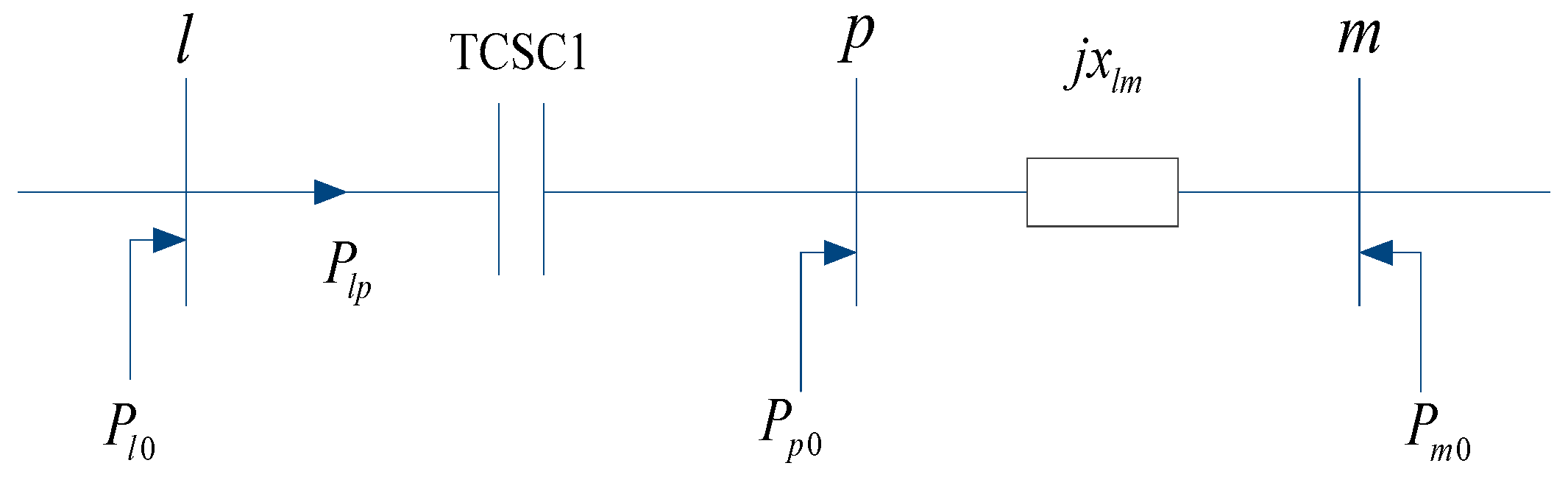
3.1. APSSR Incorporating a Single TCSC
3.2. APSSR Incorporating Double TCSCs
4. Feasibility Analysis of the Proposed Method for the System with Multiple TCSCs
- (1)
- The feasibility of the proposed method is theoretically not affected by the number of TCSCs. Of course, with the increase of K, concrete expression of Equation (22) will be gradually complicated.
- (2)
- The computational burden of the proposed method mainly depends on the inversion of K-order matrix TsK×K(XTCSC1, …, XTCSCK). Also, the number of TCSCs is generally much smaller than the number of nodes of a power grid (i.e., K << n). Therefore, the proposed method has much higher computational efficiency compared with the existing method, by avoiding inversion of the n-order parameter matrix B(XTCSC).
5. Cases Studies
5.1. Verification of the Effectiveness of the Proposed Method
5.1.1. The Scenario with a Single TCSC
5.1.2. The Scenario with Multiple TCSCs
- (1)
- The proposed method can correctly construct the explicit expression of the APSSR, which consists of the equivalent reactance parameters of TCSCs and node active power injections.
- (2)
- The effectiveness of the proposed method is not influenced by the number of TCSCs and the values of TCSC equivalent reactances.
5.2. Effects of System Scale and the Number of TCSCs on the Computational Efficiency of the Proposed Method
- (1)
- Method 1: The existing method via inversion of parameter matrix B(XTCSC)
- (2)
- Method 2: The proposed method
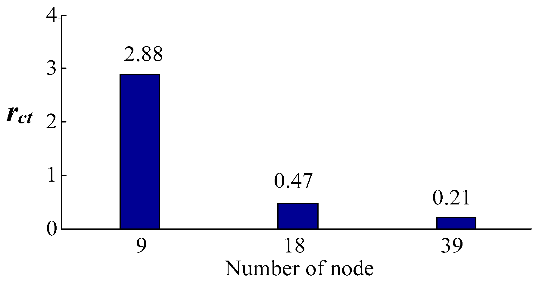
5.2.1. The Effect of System Scale
- (1)
- When node number increases, the computing times of both Method 1 and Method 2 increase.
- (2)
- Compared with the proposed Method 2, the computing time of Method 1 increases much faster.
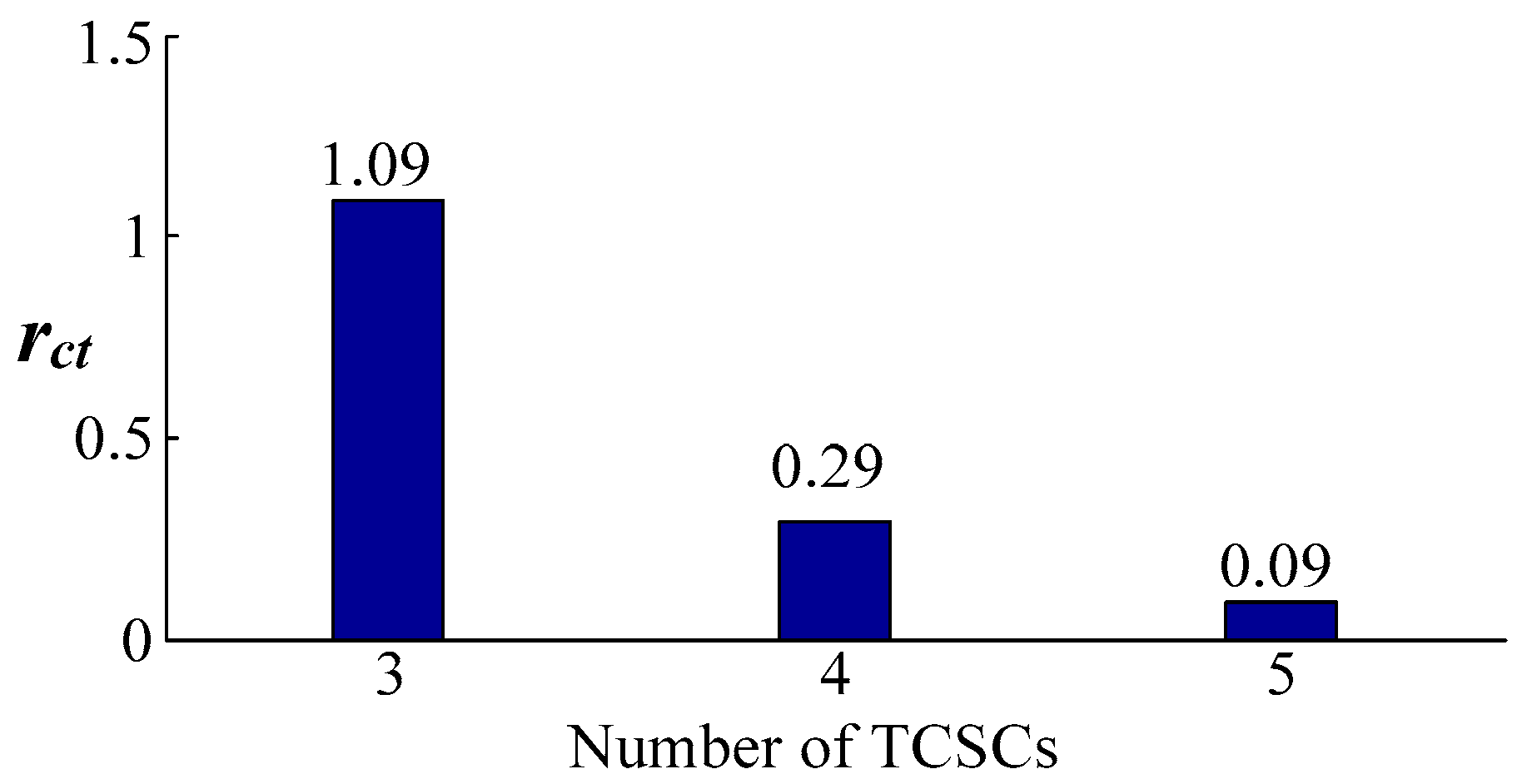
5.2.2. The Effect of the Number of TCSCs
- (1)
- When the number of TCSCs increases, the computing times of both Method 1 and Method 2 increase.
- (2)
- Compared with the proposed Method 2, the computing time of the proposed Method 1 increases much faster.
6. Conclusions
- (1)
- It can correctly construct an explicit expression of the APSSR, which consists of the equivalent reactance parameters of TCSCs and node active power injections.
- (2)
- It is suitable for a system with a single TCSC, two TCSCs, and multiple TCSCs. That is, its feasibility is not influenced by the number of TCSCs.
- (3)
- Compared with the conventional method, it shows much higher efficiency in constructing explicit expressions of APSSRs incorporating the equivalent reactance parameters of TCSCs. Moreover, the larger the system scale or the greater the number of TCSCs, the more significant the superiority in computational efficiency the proposed method is.
Acknowledgments
Author Contributions
Conflicts of Interest
References
- Charles Smith, J.; Michael, R.M.; Edgar, A.D.; Brian, P. Utility wind integration and operating impact state of the art. IEEE Trans. Power Syst. 2007, 22, 900–908. [Google Scholar] [CrossRef]
- Miao, F.; Vijay, V.; Gerald Thomas, H.; Raja, A. Probabilistic power flow studies for transmission systems with photovoltaic generation using cumulants. IEEE Trans. Power Syst. 2012, 27, 2251–2261. [Google Scholar]
- Saber, T.; Miadreza, S.; Fei, W.; Jamshid, A.; Catalão, J.P.S. Optimal scheduling of demand response in pre-emptive markets based on stochastic bilevel programming method. IEEE Trans. Ind. Electron. 2018, PP, 1. [Google Scholar] [CrossRef]
- Juan, M.M.; Juan, P. Point Estimate Schemes to Solve the Probabilistic Power Flow. IEEE Trans. Power Syst. 2007, 22, 1594–1601. [Google Scholar]
- Luo, J.; Shi, L.; Yao, L. A Multi-objective Optimization Model for Active Power Steady-state Security Region Analysis Incorporating Wind Power. In Proceedings of the IEEE Power and Energy Society General Meeting, Boston, MA, USA, 17–21 July 2016; pp. 1–5. [Google Scholar]
- Hnyilicza, E.; Lee, S.T.Y.; Schweppe, F.C. Steady-state security regions: Set-theoretic approach. In Proceedings of the Power Industry Computer Applications Conference, New Orleans, LA, USA, 2–4 June 1975; pp. 347–355. [Google Scholar]
- Wu, F.F.; Kumagai, S. Steady-state security regions of Power System. IEEE Trans. Circuits Syst. 1982, 29, 703–711. [Google Scholar] [CrossRef]
- Zhu, J. Optimization of Power System Operation, 2nd ed.; Wiley-IEEE Press: Piscataway, NJ, USA, 2015. [Google Scholar]
- Yu, Y.; Feng, F. Active power steady-state security region of power system. Sci. China Ser. A-Technol. Sci. 1990, 6, 664–672. [Google Scholar]
- Yu, Y.; Qin, C. Security region based security-constrained unit commitment. Sci. China Technol. Sci. 2013, 56, 2732–2744. [Google Scholar] [CrossRef]
- Yu, Y.; Wang, Y. Security region based real and reactive power pricing of power system. Sci. China Ser. E-Technol. Sci. 2008, 51, 2095–2111. [Google Scholar] [CrossRef]
- Alhabib, B.; Yu, Y.; Sun, G. Security region based real and reactive power optimization of power systems. Proc. CSEE 2006, 26, 1–10. [Google Scholar]
- Mohsen, H.S.; Gholamreza, A.M.; Ehsan, D.; Navid, R.A.; Abbas, K. Application of brain emotional learning-based intelligent controller to power flow control with thyristor-controlled series capacitance. IET Gener. Transm. Distrib. 2015, 9, 1964–1976. [Google Scholar]
- Duong, T.L.; Yao, J.G.; Truong, V.A. A new method for secured optimal power flow under normal and network contingencies via optimal location of TCSC. Int. J. Electr. Power Energy Syst. 2013, 52, 68–80. [Google Scholar] [CrossRef]
- Sundar, K.S.; Ravikumar, H.M. Selection of TCSC location for secured optimal power flow under normal and network contingencies. Int. J. Electr. Power Energy Syst. 2012, 34, 29–37. [Google Scholar] [CrossRef]
- Abdel-Moamen, M.A.; Padhy, N.P. Power flow control and transmission loss minimization model with TCSC for practical power networks. In Proceedings of the IEEE Power Engineering Society General Meeting, Toronto, ON, Canada, 13–17 July 2003; pp. 1–5. [Google Scholar]
- Anderson, P.M.; Fouad, A.A. Power System Control and Stability, 1st ed.; Iowa State University Press: Ames, IA, USA, 1977. [Google Scholar]
- Pai, A. Energy Function analysis For Power System Stability, 2nd ed.; Kluwer Academic Publishers: Norwell, MA, USA, 1989. [Google Scholar]
- Thorp, J.S.; Wang, H.Y. Computer Simulation of Cascading Disturbances in Electric Power Systems; University of Wisconsin: Madison, WI, USA, 2001. [Google Scholar]


| m | kdm | em | m | kdm | em |
|---|---|---|---|---|---|
| 1 | 0.6847 | −0.0767 | 20 | 0.4221 | −0.0183 |
| 2 | 0.6847 | −0.0356 | 21 | 0.4221 | −0.0183 |
| 3 | 0.7183 | −0.0235 | 22 | 0.4221 | −0.0183 |
| 4 | −0.0408 | −0.0089 | 23 | 0.4221 | −0.0183 |
| 5 | −0.0063 | −0.0003 | 24 | 0.4221 | −0.0183 |
| 6 | 0 | 0 | 25 | 0.6656 | −0.0339 |
| 7 | −0.0023 | 0.0040 | 26 | 0.5939 | −0.0275 |
| 8 | −0.0035 | 0.0060 | 27 | 0.5612 | −0.0245 |
| 9 | −0.0035 | 0.0423 | 28 | 0.5939 | −0.0275 |
| 10 | 0.0326 | −0.0040 | 29 | 0.5939 | −0.0275 |
| 11 | 0.0221 | −0.0027 | 30 | 0.6847 | −0.0356 |
| 12 | 0.0326 | −0.0040 | 32 | 0.0326 | −0.0040 |
| 13 | 0.0432 | −0.0053 | 33 | 0.4221 | −0.0183 |
| 14 | 0.0704 | −0.0086 | 34 | 0.4221 | −0.0183 |
| 15 | 0.3158 | −0.0154 | 35 | 0.4221 | −0.0183 |
| 16 | 0.4221 | −0.0183 | 36 | 0.4221 | −0.0183 |
| 17 | 0.5228 | −0.0211 | 37 | 0.6656 | −0.0339 |
| 18 | 0.5974 | −0.0220 | 38 | 0.5939 | −0.0275 |
| 19 | 0.4221 | −0.0183 | 39 | 0.6847 | −0.1017 |
| kr1 | kr2 | kdl | kdp |
|---|---|---|---|
| 0.0423 | −0.1267 | −0.0035 | 0.06847 |
| m | Proposed Method | Existing Method | m | Proposed Method | Existing Method |
|---|---|---|---|---|---|
| 1 | 0.3668 | 0.3668 | 20 | 0.3462 | 0.3462 |
| 2 | 0.5371 | 0.5371 | 21 | 0.3462 | 0.3462 |
| 3 | 0.6208 | 0.6208 | 22 | 0.3462 | 0.3462 |
| 4 | −0.0775 | −0.0775 | 23 | 0.3462 | 0.3462 |
| 5 | −0.0075 | −0.0075 | 24 | 0.3462 | 0.3462 |
| 6 | 0 | 0 | 25 | 0.5251 | 0.5251 |
| 7 | 0.0143 | 0.0143 | 26 | 0.4800 | 0.4800 |
| 8 | 0.0215 | 0.0215 | 27 | 0.4595 | 0.4595 |
| 9 | 0.1720 | 0.1720 | 28 | 0.4800 | 0.4800 |
| 10 | 0.0161 | 0.0161 | 29 | 0.4800 | 0.4800 |
| 11 | 0.0109 | 0.0109 | 30 | 0.5371 | 0.5371 |
| 12 | 0.0161 | 0.0161 | 32 | 0.0161 | 0.0161 |
| 13 | 0.0212 | 0.0212 | 33 | 0.3462 | 0.3462 |
| 14 | 0.0346 | 0.0346 | 34 | 0.3462 | 0.3462 |
| 15 | 0.2520 | 0.2520 | 35 | 0.3462 | 0.3462 |
| 16 | 0.3462 | 0.3462 | 36 | 0.3462 | 0.3462 |
| 17 | 0.4354 | 0.4354 | 37 | 0.5251 | 0.5251 |
| 18 | 0.5061 | 0.5061 | 38 | 0.4800 | 0.4800 |
| 19 | 0.3462 | 0.3462 | 39 | 0.2631 | 0.2631 |
| m | Proposed Method | Existing Method | m | Proposed Method | Existing Method |
|---|---|---|---|---|---|
| 1 | −0.0359 | −0.0359 | 20 | 0.1528 | 0.1528 |
| 2 | −0.0427 | −0.0427 | 21 | 0.1528 | 0.1528 |
| 3 | −0.0695 | −0.0695 | 22 | 0.1528 | 0.1528 |
| 4 | −0.2702 | −0.2702 | 23 | 0.1528 | 0.1528 |
| 5 | −0.0373 | −0.0373 | 24 | 0.1528 | 0.1528 |
| 6 | 0 | 0 | 25 | −0.0257 | −0.0257 |
| 7 | −0.0144 | −0.0144 | 26 | 0.0262 | 0.0262 |
| 8 | −0.0216 | −0.0216 | 27 | 0.0498 | 0.0498 |
| 9 | −0.0276 | −0.0276 | 28 | 0.0262 | 0.0262 |
| 10 | 0.1927 | 0.1927 | 29 | 0.0262 | 0.0262 |
| 11 | 0.1304 | 0.1304 | 30 | −0.0427 | −0.0427 |
| 12 | 0.1927 | 0.1927 | 32 | 0.1927 | 0.1927 |
| 13 | 0.2549 | 0.2549 | 33 | 0.1528 | 0.1528 |
| 14 | 0.4156 | 0.4156 | 34 | 0.1528 | 0.1528 |
| 15 | 0.2322 | 0.2322 | 35 | 0.1528 | 0.1528 |
| 16 | 0.1528 | 0.1528 | 36 | 0.1528 | 0.1528 |
| 17 | 0.0776 | 0.0776 | 37 | −0.0257 | −0.0257 |
| 18 | 0.0215 | 0.0215 | 38 | 0.0262 | 0.0262 |
| 19 | 0.1528 | 0.1528 | 39 | −0.0318 | −0.0318 |
| Number of Nodes | Method 1/s | Method 2/s |
|---|---|---|
| 9 | 0.1353 | 0.0039 |
| 18 | 1.0700 | 0.0050 |
| 39 | 2.9307 | 0.0061 |
| Number of TCSCs | Method 1/s | Method 2/s |
|---|---|---|
| 3 | 5.2401 | 0.0571 |
| 4 | 21.8122 | 0.0630 |
| 5 | 136.9217 | 0.1227 |
© 2018 by the authors. Licensee MDPI, Basel, Switzerland. This article is an open access article distributed under the terms and conditions of the Creative Commons Attribution (CC BY) license (http://creativecommons.org/licenses/by/4.0/).
Share and Cite
Chen, R.; Lin, T.; Chen, B.; Bi, R.; Xu, X. Novel Method for Rapidly Constructing Active Power Steady-State Security Regions Incorporating the Equivalent Reactances of TCSCs. Energies 2018, 11, 551. https://doi.org/10.3390/en11030551
Chen R, Lin T, Chen B, Bi R, Xu X. Novel Method for Rapidly Constructing Active Power Steady-State Security Regions Incorporating the Equivalent Reactances of TCSCs. Energies. 2018; 11(3):551. https://doi.org/10.3390/en11030551
Chicago/Turabian StyleChen, Rusi, Tao Lin, Baoping Chen, Ruyu Bi, and Xialing Xu. 2018. "Novel Method for Rapidly Constructing Active Power Steady-State Security Regions Incorporating the Equivalent Reactances of TCSCs" Energies 11, no. 3: 551. https://doi.org/10.3390/en11030551
APA StyleChen, R., Lin, T., Chen, B., Bi, R., & Xu, X. (2018). Novel Method for Rapidly Constructing Active Power Steady-State Security Regions Incorporating the Equivalent Reactances of TCSCs. Energies, 11(3), 551. https://doi.org/10.3390/en11030551