1. Introduction
In many countries around the world, renewable energies are gradually replacing traditional energy sources, mainly because of the unprecedented and irreversible environmental damage caused by fossil and nuclear fuels and the continuing reduction of renewable technology costs [
1,
2]. Among the main sources of renewable energies, wind energy has presented an important development, being an attractive alternative in terms of its costs and low environmental impact [
3]. However, the integration of wind power into electrical systems presents several challenges due to its uncertainty and variability, as its generation depends on a stochastically-behaved primary energy resource [
4]. For example, the short-term generation scheduling of an electrical system must provide reliable estimates of how much wind power will be produced to obtain the optimal selection of dispatched units and the optimal generation levels of conventional units. Forecasting errors can increase generation costs of the system, due to the need for dispatching peak units to supply an unexpected resource shortage, which also decreases its reliability. This issue limits wind power penetration since it may put at risk the planning and economic operation of the electricity markets, as well as the safety and reliability of the power system. Therefore, forecasting tools that precisely describe and predict wind power generation behavior are critical in keeping the electricity supply economical and reliable.
Research proposals attempting to build an accurate prediction model for wind power can be divided mainly into physical methods (which use numerical weather prediction based on meteorological processes), traditional statistical methods (data-driven modeling as time series) and artificial intelligence or machine learning models [
5,
6]. From a statistical point of view, time series forecasting is a common problem in many fields of science and engineering, and different approaches can be applied in the context of wind power prediction. One of such approaches is the Autoregressive Fractionally-Integrated Moving Average (ARFIMA) methodology for fitting a class of linear time series models with long-term dependencies. However, most of those models assume linearity and stationary conditions over the time series, and these restrictions are not always met with real wind power data [
7,
8]. It is also common to find hybrid methods based on combinations of physical and statistical models, using different strategies [
6], where basically the statistical model operates as a complement of the physical models using the data generated by some numerical weather prediction.
In recent years, more complex techniques from the area of Artificial Intelligence (AI) have gained popularity. Specifically, from the machine learning community (sub-area of AI), we can find proposals using different models such as support vector machines, random forests, clustering, fuzzy logic and artificial neural networks, among others. Particularly, Artificial Neural Networks (ANN) have shown good performance, surpassing various state of the art techniques [
9]. Nevertheless, most of those approaches are based on univariate time series without considering exogenous variables. Thus, adding characteristics of the studied phenomenon could improve the models performance [
10,
11].
Recurrent Neural Networks (RNN) are a particular class of ANN that is gaining increased attention, since they can model the temporal dynamics of a series in a natural way [
12]. The process of constructing the relationships between the input and output variables is addressed by certain general purpose learning algorithms. An RNN is a neural network that operates over time. At each time step, an input vector activates the network by updating its (possibly high-dimensional) hidden state via non-linear activation functions and uses it to make a prediction of its output. RNNs form a rich class of models because their hidden state information is stored as high-dimensional distributed representations (as opposed to a hidden Markov model, whose hidden state is essentially log n-dimensional). Their nonlinear dynamics allow modeling and forecasting tasks for sequences with highly complex structures. Some drawbacks of the practical use of RNN are the long time consumed in the modeling process and the large amount of data required in the training process. Furthermore, the process of learning the weights of the network, by means of a gradient descent-type optimization method, makes it difficult to find the optimal values of the model. To tackle some of these problems, two recurrent network models, named Long Short-Term Memory (LSTM) and Echo State Networks (ESN), have been proposed.
This paper addresses the problem of predicting wind power with a forecast horizon from 1–48 h ahead, by devising a neural network that uses LSTM memory blocks as units in the hidden layer, within an architecture of the ESN type. The proposal has two stages: (i) first, the hidden layer is trained by the gradient descent-based algorithm, using the input as the target, inspired by a classic autoencoder to extract characteristics automatically from the input signal; (ii) second, only the output layer weights are trained by a regularized quantile regression; this reduces the cardinality of the hypothesis space, where it might be easier to find a consistent hypothesis. The advantages of this proposal are three-fold: (i) the design of the memory blocks that store and control the information flowing through the hidden layer; (ii) the sparsely-connected recurrent hidden layer of the ESN that contains fewer features and, hence, is less prone to overfitting; (iii) adjusting the weights with quantile regression provides a more robust estimation of wind power.
The proposal is evaluated and contrasted with data provided by the wind power forecasting system developed at Technical University of Denmark (DTU): the Wind Power Prediction Tool (WPPT). This system predicts the wind power production in two steps. First, it transforms meteorological predictions of wind speed and wind direction into predictions of wind power for a specific area using a power curve-like model. Next, it calculates an optimal weight between the observed and the predicted production in the area, so that the final forecast can be generated. For more details, please refer to [
13].
In summary, the proposed model uses historical wind power data and meteorological data provided by a Numerical Weather Prediction (NWP) system. This forecasting technique does not make a priori assumptions about the underlying distribution of the process generated by the series, and it incorporates meteorological variables that improve the predictions.
The paper is organized as follows:
Section 2 describes general techniques for wind power forecasting;
Section 3 provides a brief description of RNN, specifically focusing on LSTM and ESN;
Section 4 presents the details of the proposed model;
Section 5 provides a description and preprocessing of the dataset used, the metrics used to evaluate the forecasting accuracy and the experimental study used to validate the proposed model; finally,
Section 6 presents the conclusions.
3. Recurrent Neural Networks
A recurrent neural network [
41,
42] is a type of artificial neural network where the connections of its units (called artificial neurons) present cycles. These recurrent connections allow one to describe targets as a function of inputs at previous time instants, this being the reason it is said that the network has “memory”. Hence, the network can capture the temporal dynamic of the series [
12]. Formally, under a standard architecture [
43], it can be defined as: given a sequence of inputs
, each in
, the network computes a sequence of hidden states
, each in
, and a sequence of predictions
, each in
, by iterating the equations:
where
,
and
are the weight matrices of the input layer, hidden layer and output layer, respectively;
and
are the biases,
and
are pre-defined vector valued functions, which are typically non-linear with a well-defined Jacobian. A predefined value
is set as the state of the network. The objective function associated with an RNN for a single
pair is defined as
, where
is the model parameters vector and
L is a distance function that measures the deviation of the prediction
from the target output
(e.g., the squared error). The overall objective function for the whole training set is simply given by the average of the individual objectives associated with each training example [
44].
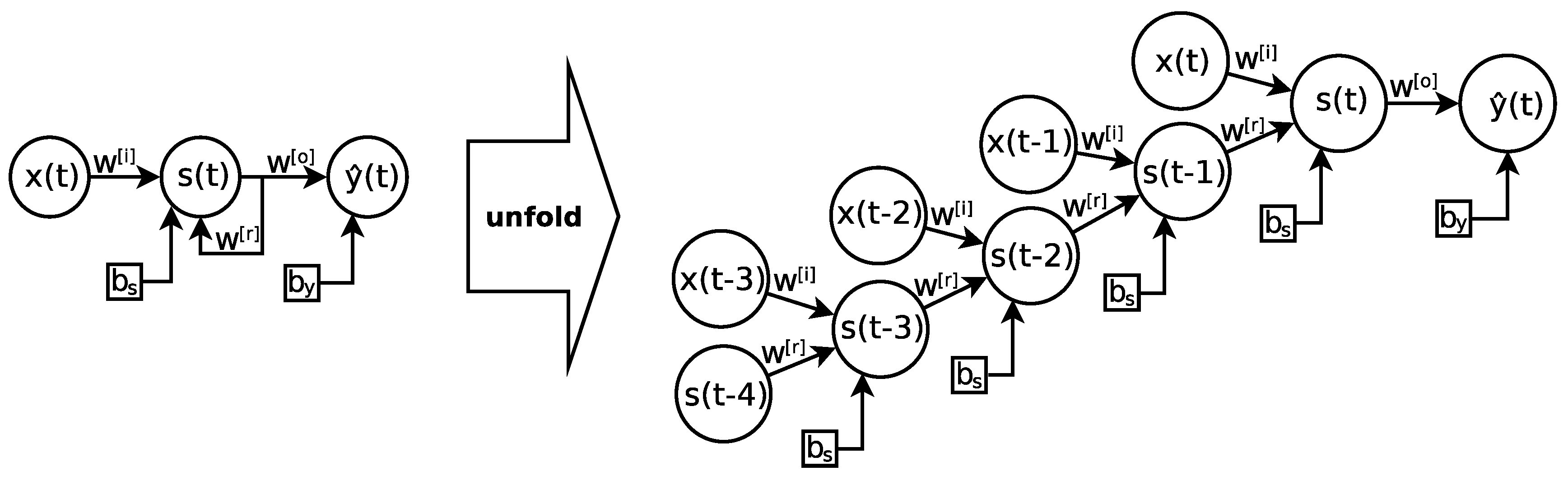
Despite its advantages, this type of network suffers from the problem of “vanishing/exploding gradient” [
45], which produces the effect of making the training of the hidden layers more difficult the closer they are to the input layer, which in turn hinders learning the underlying patterns. Since data flow over time, an RNN is equivalent to a multi-layered feedforward neural network, as shown in
Figure 1. That is, it is possible to unfold the recurrent network
l times into the past, resulting in a deep network with
l hidden layers.
Recently, different RNN variants have tried to solve this problem, Long Short-Term Memory (LSTM) and Echo State Networks (ESN) becoming the most popular approaches.
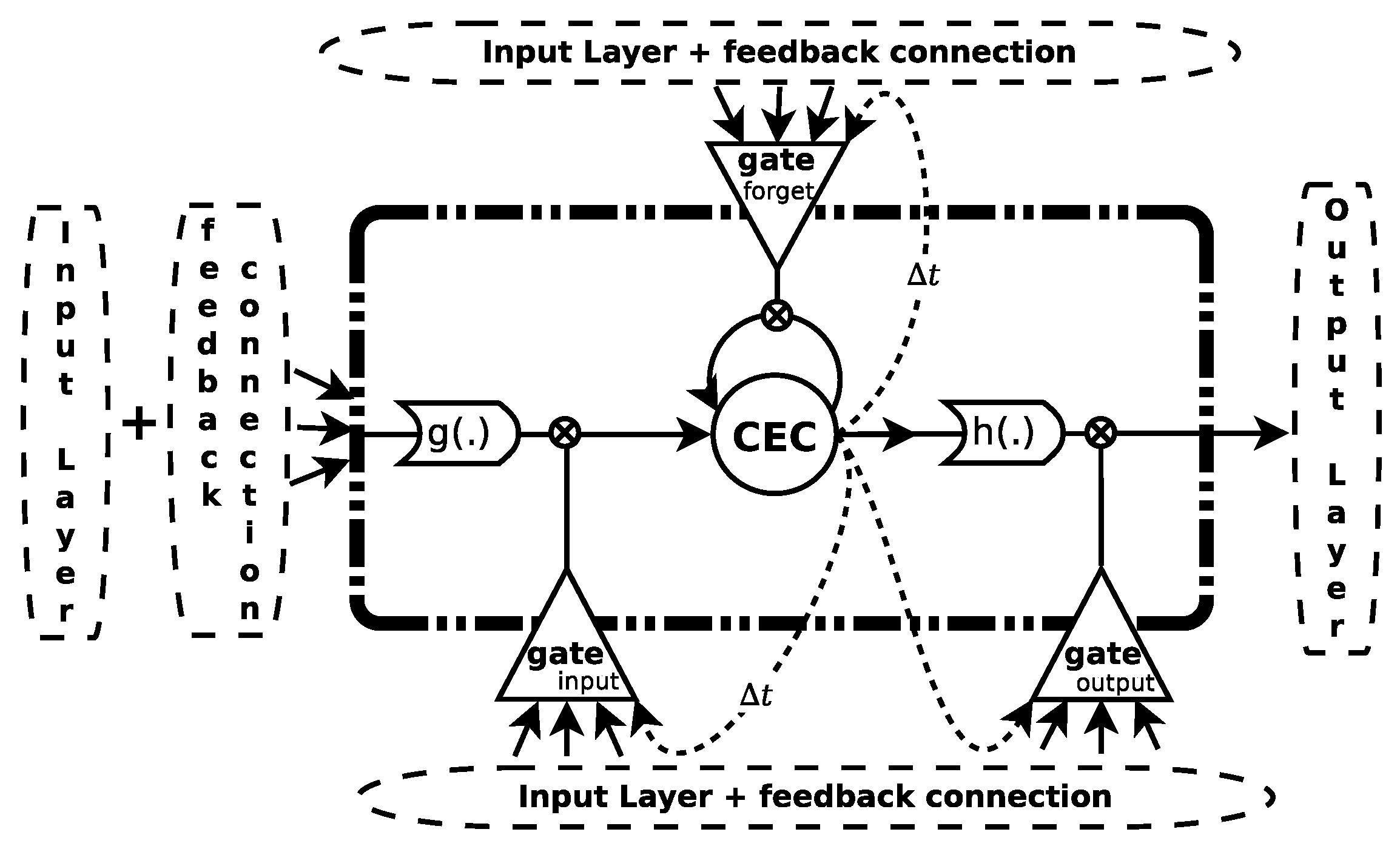
3.1. Long Short-Term Memory
This model replaces the traditional neuron of the perceptron with a memory block (see
Figure 2). This block generally contains a memory cell and some “gateways” (sigmoidal activation functions in the range [0,1]) that control the information flow passing through the cell. Each memory cell is a self-connected linear unit called the “Constant Error Carouse ” (CEC), whose activation is considered the state of the cell. This new network is known as Long Short-Term Memory [
39].
The CEC mitigates the vanishing (exploding) problem of the gradient, since the backward flow of the local error remains constant within the CEC, without increasing or decreasing as long as no new input or external error signal is present. The training of this model is based on a modification of both the backpropagation through time [
46] and real-time recurrent learning [
47] algorithms. Let
,
and
be linear combinations of the inputs weighted with the weights for the different gates (input, forget and output, respectively) at time
t for block
j. Let
,
and
be the outputs of the activation functions for each gate. Let
be the weighted entry to the block
j and
the cell state at time
t. Let
be the output of the
j-th block. Then, the information flow forward is expressed as:
where
is the weight that connects unit
m to unit
j and the super index indicates to which component of the block it belongs. Additionally
indicates recurrent weights, and
indicates direct weights between the cell and a particular gate;
is the input signal to the
m-th neuron of the input layer;
is the output of the
m-th block in time
;
,
and
are sigmoidal activation functions in the range [0,1], [−2,2] and [−1,1], respectively. For a more detailed study of this model, please refer to [
48].
3.2. Echo State Networks
Another type of recurrent network comes from the paradigm Reservoir Computing (RC) [
49], a field of research that has emerged as an alternative gradient descent-based method. The key idea behind reservoir computing is to use a hidden layer formed by a large number of sparsely-connected neurons. This idea resembles kernel methods [
50], where input data are transformed to a high-dimensional space in order to perform a particular task.
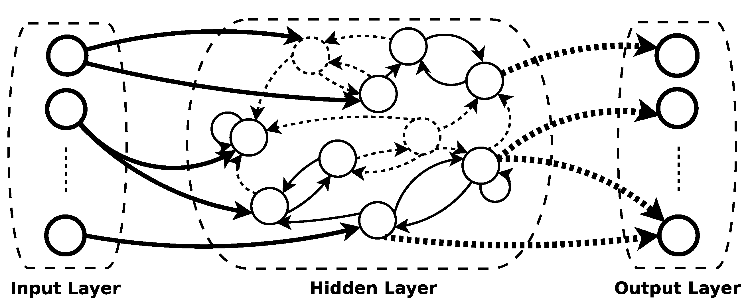
One of the pioneering models within this field is known as the Echo State Network (ESN) [
40]. The model, in a practical sense, is very simple and easy to implement: it consists of three layers (input, hidden and output), where the hidden layer (reservoir) is formed by a large number of neurons (∼1000) and randomly connected with a low connectivity rate between them (allowing self-connections) (see
Figure 3).
The novelty of this model is that during the training phase, the weights of the connections within the reservoir are not updated, and only the output layer is trained (the weights that connect the reservoir with the last layer), usually by means of ridge regression [
51]. Then, the reservoir acts as a non-linear dynamic filter that temporarily maps the input to a high-dimensional space, without training the hidden layer weights.
Let r be the number of neurons in the reservoir; an matrix with the weights of the reservoir connections; an array , where k is the number of neurons in the output layer and n the number of neurons in the input layer. When designing an ESN, a spectral radius of close to one (the maximum proper value in absolute value) must be ensured. In order to do this, the weight matrix must be pre-processed using the following steps:
Here,
is the spectral radius of
, and therefore, the spectral radius of
is equal to
. Since the spectral radius determines how fast the influence of an input
vanishes through time in the reservoir, a larger
value is required for tasks that need longer memory [
52].
In addition, the neuron outputs of the reservoir (known as states) are obtained by the following expression:
where
is the output of a hidden neuron at time
t,
is a “leaking rate” that regulates the update speed in the dynamics of the reservoir,
is an activation function and
is a linear combination of the input signals. Since the states are initialized to zero,
, it is necessary to set an amount of
points in the series
to run the network and initialize the internal dynamics of the reservoir. If
is a matrix
with the states of all hidden layer neurons for
, then the following matrix equation calculates the weights of the output layer:
where
is the transpose of
,
is a regularization parameter,
is an identity matrix and
is a
matrix with the actual outputs, that is
.
Additionally, in order to obtain prediction intervals, in [
53], an ESN ensemble is proposed using Quantile Regression (QR) [
54] to calculate the output layer weights of each network. This technique is supported by the fact that quantiles associated with a random variable
Y, of order
, are position measures that indicate the value of
Y to reach a desired cumulative probability
, that is,
where
corresponds to the order quantile
. For example, the median is the best known quantile and is characterized as the value
that meets
.
Then, quantile regression proposes that
is written as a linear combination of some known regressors and unknown coefficients, analogous to modeling the conditional mean by using a multiple linear regression, that is,
where
and
K are called regressors (explanatory variables) and
are the unknown coefficients based on
, which is determined from a set of observations
. The loss function to be minimized to find the coefficients
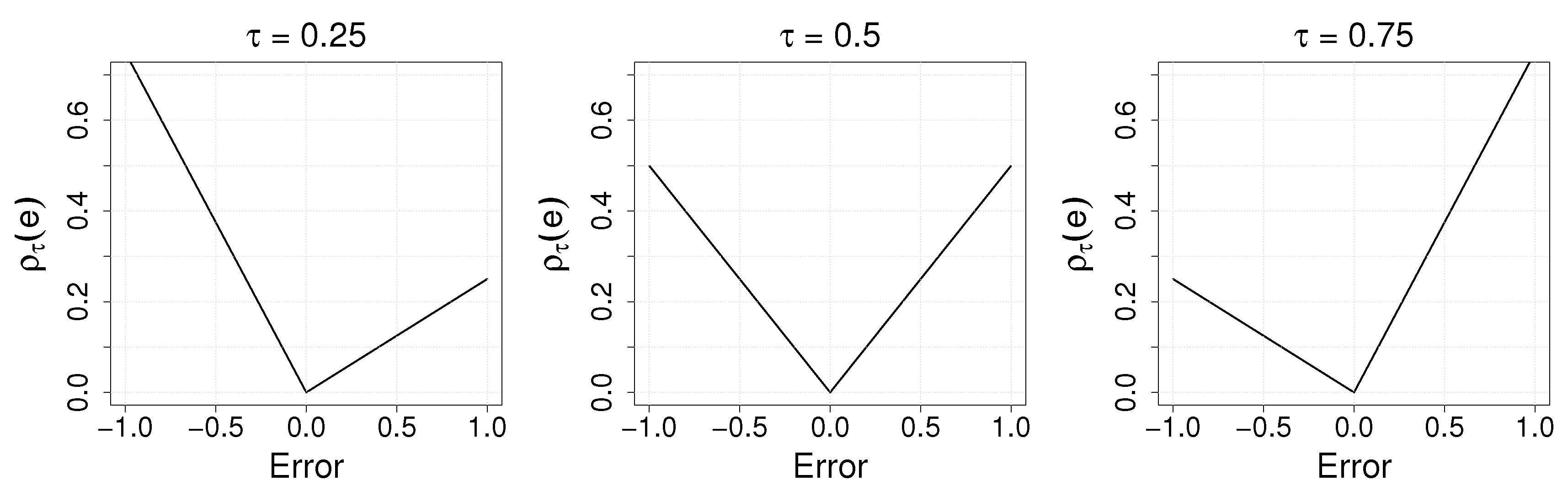
is defined by:
where
is the error between the variable
y and the
-th desired quantile
q.
Figure 4 shows the loss function
for different
values. Then, the
-conditional quantile can be found by looking for the parameters
that minimize:
4. LSTM+ESN Proposed Model
Despite the fact that the LSTM has shown good performance in forecasting [
55,
56], its training process can be computationally expensive, due to the complexity of its architecture. As a consequence, the computational training cost increases as the number of blocks increases. In addition, it might overfit depending on the values of its hyperparameters such as the number of blocks, the learning rate or the maximum number of epochs.
On the other hand, good performance has also been reported for the ESN [
57,
58]; however, it is possible to improve its results by adjusting the hidden layer weights (sacrificing its simplicity). An example is the work of Palangi [
59], where all the weights of the network are learned. The proposal exhibited improvement over the traditional ESN, tested in a phone classification problem on the TIMIT dataset.
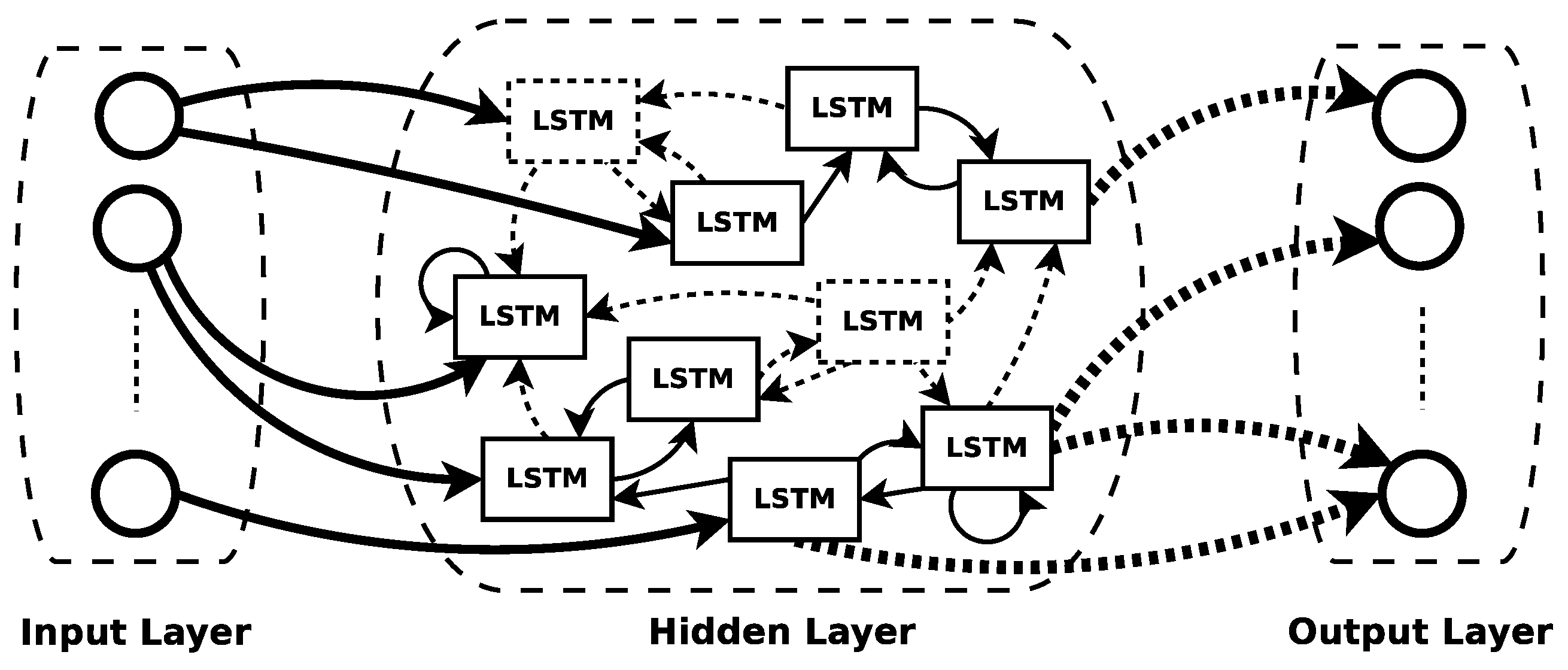
Inspired by the advantages of both networks, we propose a novel neural network called LSTM+ESN, a recurrent neural network model based on the architecture of an ESN using as hidden neurons LSTM units (see
Figure 5). Following the work of Gers [
48], all the layers are allowed to be trained using truncated gradients, but with some restrictions imposed by the ESN architecture.
Let M be the number of input neurons, J the number of blocks in the hidden layer and K the number of neurons in the output layer. Let be an matrix with the weights connecting the input layer to the input of the blocks; , , are matrices with the weights of the connections from the input layer to the input, forget and output gates, respectively. Let be a matrix with the weights of the recurrent connections between the blocks of the hidden layer. , , are matrices with the weights of the connections from the recurring signals of the outputs of the blocks to the input, forget and output gates, respectively. Let , , be matrices with the weights that directly connect the CEC with their respective input, forget and output gates. Let , , , be row vectors of dimension J with the weights bias associated with the entry of each block, input gate, forget and output, respectively. Let be a vector with the CEC states for each block of the hidden layer at instant t.
Let be a matrix with the weights of the output layer, where if there is a direct connection from the layer input with the output, otherwise. Let be a vector with the entry for the output layer at time t.
To train this architecture, it is necessary to include all the steps described in Algorithm 1.
| Algorithm 1 LSTM+ESN training scheme |
| 1: Dataset is split in two: for training and for validating. |
| 2: Randomly initialize sparse hidden weights matrices , , and from a uniform distribution with range (−0.1, 0.1). |
| 3: Initialize hidden weight matrices , , , , , , , , , and from a uniform distribution with range (−0.1, 0.1). |
| 4: Set as or . |
| 5: Set the value for Regularization. |
| 6: TrainNet_by_LSTM() |
| 7: TrainNet_by_ESN(, Regularization) |
| 8: repeat |
| 9: TrainNet_by_LSTM() |
| 10: TrainNet_by_ESN(, Regularization) |
| 11: until Convergence using the validation set as the early stopping condition. |
In order to update the matrices initialized in Steps 2 and 3, Step 6 chooses the weight matrices that minimize the error of the LSTM output with respect to a vector with the expected target at instant
t,
, defined as
and set in Step 4. Here,
can be the real target
(in order to learn the original output) or the input
in order to learn a representation of the original input resembling the classic autoencoder approach. The loss function is defined to minimize the mean square error “online” (at each instant
t) given by Equation (
6):
Then, the gradient associated with
is given by the following equation:
where ⊙ represents the element-to-element multiplication between matrices or vectors and
represents the derivative of the activation function associated with the output neurons. If we consider that
, we can write:
Then, the gradients for the other weight matrices are:
where
are the different matrices associated with the forget gate,
represents the vector with the inputs of each
.
is the transpose of the vector with all the inputs of the forget gate,
represents the matrix with all the weights associated with the forget gate,
is the derivative of the activation function of the gates and
is the matrix with the weights that connects only the hidden layer with the output layer.
here,
and
is the element-wise product of a vector with each row of a matrix, i.e.,
Algorithm 2, called
TrainNet_by_LSTM, systematically describes Step 3 of Algorithm 1, used to train the network. First, the network is trained online with the AdaDelta [
60] optimization algorithm as in the LSTM training, using only one epoch (Step 6). We choose this optimization technique because it has been shown that it converges faster than other algorithms of the descending gradient type [
61]. In addition, to preserve the imposed requirements of the ESN reservoir, after each weight update, the matrix of recurring connections is kept sparse by zeroing out those weights that were initially set as zero (Step 7). In order to avoid producing diverging output values when updating the output weights or the influence of the LSTM gates being biased by some very large weights, a filter is applied that resets to zero weights that exceed a threshold
(Step 10 and Step 12). Since online training is performed, the matrix of recurring connections will be re-scaled to maintain a spectral radius
at each instant
t. The parameter
MaxEpoch indicates the maximum number of epochs to use;
means the maximum value that can take the weights;
fixedWo indicates if the output weights are updated or not;
keepSR indicates if the spectral ratio is kept or not; and
cleanHW controls if the weights that exceed
are reset to zero.
| Algorithm 2 TrainNet_by_LSTM() |
| Input: A set of instances |
| Input: MaxEpoch = 1, , fixedWo=False, keepSR=True, cleanHW=True |
| 1: Define |
| 2: while MaxEpoch do |
| 3: |
| 4: for T do |
| 5: ForwardPropagate(, network) |
| 6: UpdateWeights(, , network) |
| 7: Sparse connectivity is maintained by setting the inactive weights back to zero. |
| 8: if cleanHW == True then |
| 9: if fixedWo == False then |
| 10: ssi |
| 11: end if |
| 12: ssi , output layer |
| 13: end if |
| 14: end for |
| 15: if keepSR == True then |
| 16: |
| 17: end if |
| 18: end while |
| Output: Net’s Weights |
Later, in order to update the output layer weights
, the weights that solve the multi-linear regression
are chosen in Step 4 of Algorithm 1, called
TrainNet_by_ESN(). This can be done, for example, using ridge regression as in Equation (
2) or by means of quantile regression [
54]. The latter approach gets a more robust estimation of
. Recall that the model needs to use a regularized regression because
is a singular matrix. Currently, there are different alternatives in the literature to do this, but for this proposal, we used a regularized quantile regression model based on an elastic network, implemented in the R-project package
hqreg.
At last, a fine tuning stage is carried out in two steps: (i) TrainNet_by_LSTM is performed using as the target output; (ii) TrainNet_by_ESN is performed using the same regression as in Step 7 from Algorithm 1.
Both steps are repeated until early stopping conditions using are met.
Thus, the LSTM+ESN architecture can lead to different variants depending on the way that is chosen in Step 4, Algorithm 1, and the parameter regressionis set in Step 5, Algorithm 1. For instance, LSTM+ESN+Y+RR denotes the LSTM+ESN architecture trained with as a target in Step 4 and Ridge Regression in Step 5.
In this work, we use LSTM+ESN, training the hidden layer using
as in the autoencoder and Ridge Regression (LSTM+ESN+X+QR) for wind power forecasting, since extracting a representation of the original input and taking advantage of the robustness of QR might improve prediction performance. However, in
Section 5, we assess the proposal against other LSTM+ESN architecture variants.
Algorithm 3 corresponds to a detailed version of Algorithm 1 describing the particular setting LSTM+ESN+X+QR that we use in this work. The parameter validate indicates if the input dataset is split or not in dataset-valid and dataset-train; MaxEpochGlobal indicates the maximum number of epochs in the fine tuning stage; and Regularization refers to the regularization used by the TrainNet_by_ESN step; which in this case is always set to QR.
| Algorithm 3 LSTM+ESN+X+QR |
| Input: A set of instances . |
| 1: validate=True, MaxEpochGlobal = 1, Regularization = QR |
| 2: |
| 3: if validate == True then |
| 4: |
| 5: |
| 6: end if |
| 7: TrainNet_by_LSTM() |
| 8: TrainNet_by_ESN(,Regularization) |
| 9: if validate == True then |
| 10: CalculateForecastError() |
| 11: end if |
| 12: Save(network) |
| 13: Define , attempts=1, MaxAttemtps=10 |
| 14: whileMaxEpochGlobal do |
| 15: |
| 16: RestartOutputs(network) |
| 17: RestartGradients(network) |
| 18: TrainNet_by_LSTM(; fixedWo=True) |
| 19: if validate == True then |
| 20: TrainNet_by_ESN(,Regularization) |
| 21: CalculateForecastError() |
| 22: if then |
| 23: |
| 24: Save(network) |
| 25: else |
| 26: attempts←attempts + 1 |
| 27: end if |
| 28: else |
| 29: Save(network) |
| 30: end if |
| 31: if attempts>MaxAttemtps then |
| 32: break |
| 33: end if |
| 34: end while |
| 35: LoadSavedNet() |
| 36: TrainNet_by_ESN() |
| Output: Last network saved |
5. Experiments
5.1. Data Description and Preprocessing
In order to assess the proposed models, we used data from the Klim Fjordholme wind farm [
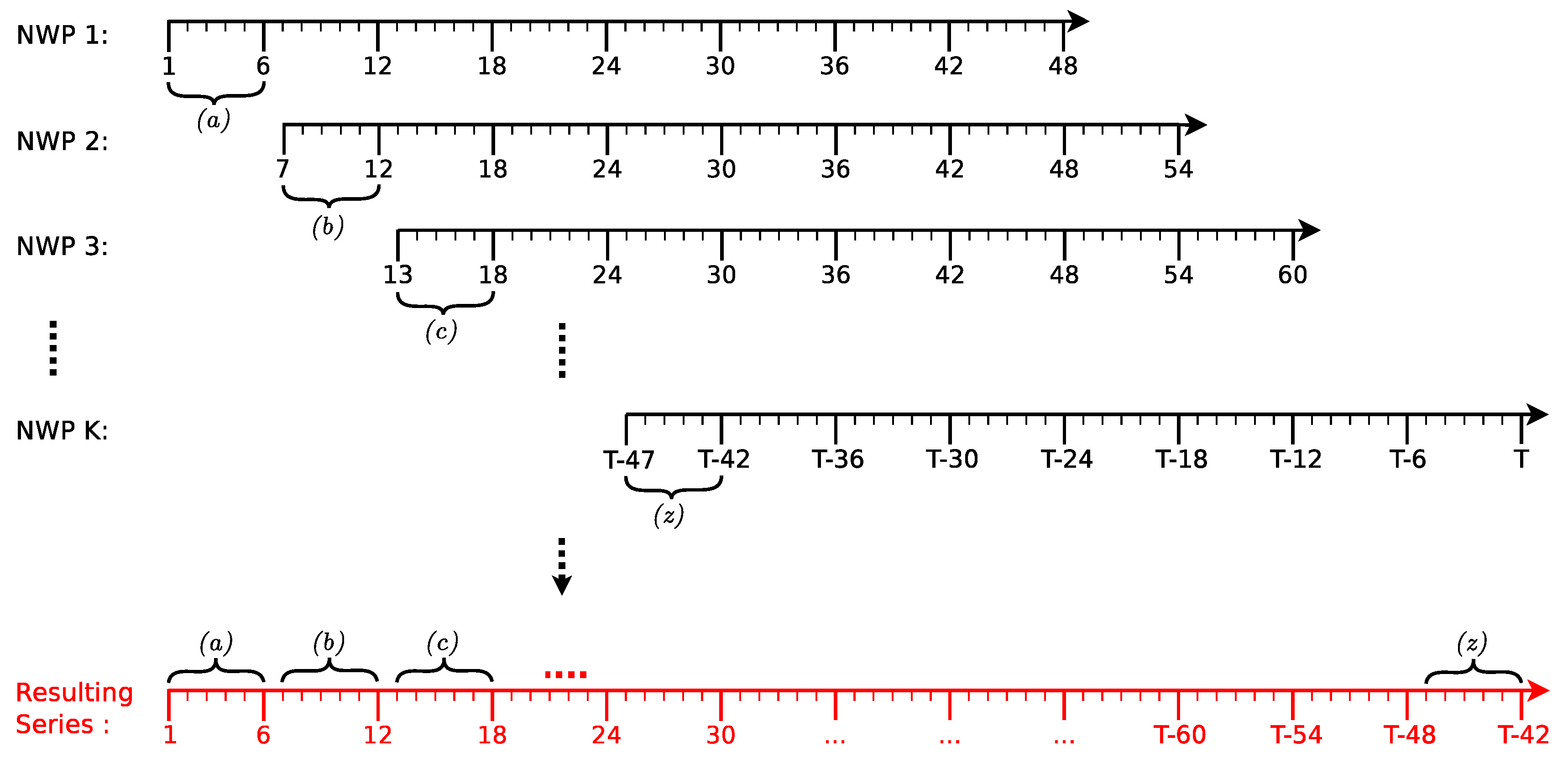
62] that consists of generated power measurements and predictions of several meteorological variables such as wind speed, wind direction and ambient temperature, generated by the HIRLAM model: a NWP system that is used by the Danish Meteorological Institute. These predictions are made 48 h ahead every 6 h, and they might present missing values. To avoid overlapping of the predictions (as depicted in
Figure 6), a resulting series (in red) is generated, only considering the first six points of each forecast.
An RNN-based model is not capable of working with missing data. A missing value is imputed by means of a linear interpolation on and plus an additive Gaussian noise . In addition to the aforementioned characteristics, to increase the performance of our proposal, we add the date of each record using three variables: (month, day and hour). Given the above, the input vector at each time step t is a lag one vector composed of the following characteristics: wind speed, wind direction, temperature, month, day, hour and wind power. All features were normalized to the range using the min-max method. Finally, the resulting series is composed of 5376 observations from 00:00 on 14 January 2002 to 23:00 on 25 August 2002.
5.2. Forecasting Accuracy Evaluation Metrics
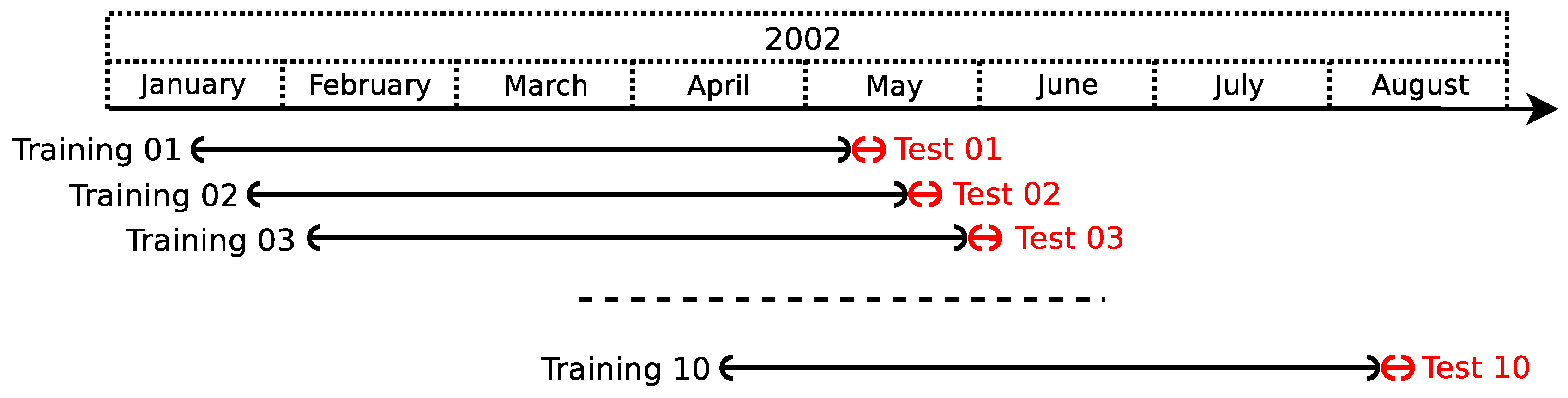
In order to assure generalization capabilities for the proposed model, the time series is divided into
subseries, and the performance of the model is evaluated in each of them; analogous to what is done when performing cross-validation to test a model performance. Each subseries is generated using a sliding window of approximately 111.96 days (approximately 3.7 months), with a step size of approximately 10 days that slides over the original series, as shown in
Figure 7.
The performance of the models is measured on the prediction of 48 h and then averaged over the subseries in order to get a global measure. These predictions are generated using the multi-stage approach [
63]. For a single subseries
r, different evaluation metrics are used based on the error
at
h steps ahead, defined as:
where
is the desired output at instant
,
T is the index of the last point of the series used during training,
h is the number of steps ahead, from 1–48, and
is the estimated output at time
generated by the model.
The metrics to be used are the Mean Squared Error (MSE), the Mean Absolute Error (MAE), the Mean Absolute Error Percentage (MAPE) and the Standard Deviation of Error (SDE) defined as follows:
where MSE(
h) and MAE(
h) are the MSE and MAE for each
h step ahead, respectively,
H indicates the maximum number of steps ahead and the subindex
r indicates the used subseries.
The hyperparameters settings where selected using one of the following criteria:
s1: the one that achieves the lowest MSE averaged over every subseries and every step ahead of the test set, as in Equation (
22).
s2: the one that achieves the lowest weighted average of:
where and . Hence, errors from predictions closer to the last value are used as the training weight more than those further ahead.
5.3. Case Study and Results
In this section, we compare our proposal against a persistence model, the forecast generated by the Wind Power Prediction Tool (WPPT) [
62], and some variants of the LSTM+ESN framework: the first trains the hidden layer using
as target and uses ridge regression instead of quantile regression (LSTM+ESN+Y+RR); the second one trains the hidden layer using
as in the autoencoder and ridge regression (LSTM+ESN+X+RR); and the third one trains the hidden layer using
as the target and quantile regression (LSTM+ESN+Y+QR). Each of the variants may use either s1 or s2 selection criterion, for example, LSTM+ESN+Y+QR+s1 would denote the third variant using s1 criterion. S. is used when choosing either criterion obtains the same hyperparameters values.
The configuration of the hyperparameters for the algorithms used in the LSTM+ESN models are shown in
Table 1,
Table 2 and
Table 3.
The other parameters are tuned according to the following scheme: First, we tune the number of blocks of the hidden layer , keeping fixed the spectral radius and the regularization parameter , using either s1 or s2 as the selection criterion. Next, and are tuned, selecting both parameters always by means of the s1 criterion.
Moreover, the identity function was used as the output layer activation function. Direct connections were also used from the input layer to the output layer, but these connections were omitted when using Algorithm 2 the first time (Step 7 of Algorithm 3). Matrices are generated sparsely, having the same positions for their zero values, since recurrent connection between unit i and unit j is represented by the values coming from the four recurrent matrices. Non-zero weights of each matrix are generated from a uniform distribution , independently of each other. Sparse arrays were also used when connecting the input layer with the hidden layer, that is and .
Table 4 shows the parameter tuning for different LSTM+ESN variants. The ID column shows a short name for the model, used hereinafter. Now, we assess the following models: persistence, WPPT, and LSTM+ESN variants
Is it important to mention that, since WPPT presents missing values in its forecasting, the error is calculated only for those points present in the WPPT forecast.
Table 5 shows the global results averaging over all subseries. The symbol * indicates when the corresponding algorithm outperforms WPPT. Best results are marked in bold.
Results show that M6 outperforms both M1 and WPPT, in all metrics. Besides, M1 exhibits worse performance than WPPT in terms of MAE, MAPE and SDE. Since M1 does not use either QR or the autoencoder inspired approach, we can note that both artifacts improve the performance of the LSTM+ESN network. A similar behavior is detected when comparing M7 with WPPT: M7 is better than WPPT in all metrics except in SDE.
On the other hand, our proposal is also better in all metrics than both M2 and M3, both of which include the autoencoder idea, but without using QR. This suggests that by using a robust Y estimation on automatically-extracted features, better performance is achieved. Our proposal also performs better when compared with both M4 and M5, both of which use QR, but without automatic extraction of features. This indicates that it is not enough to use a robust estimation method to achieve a lower error.
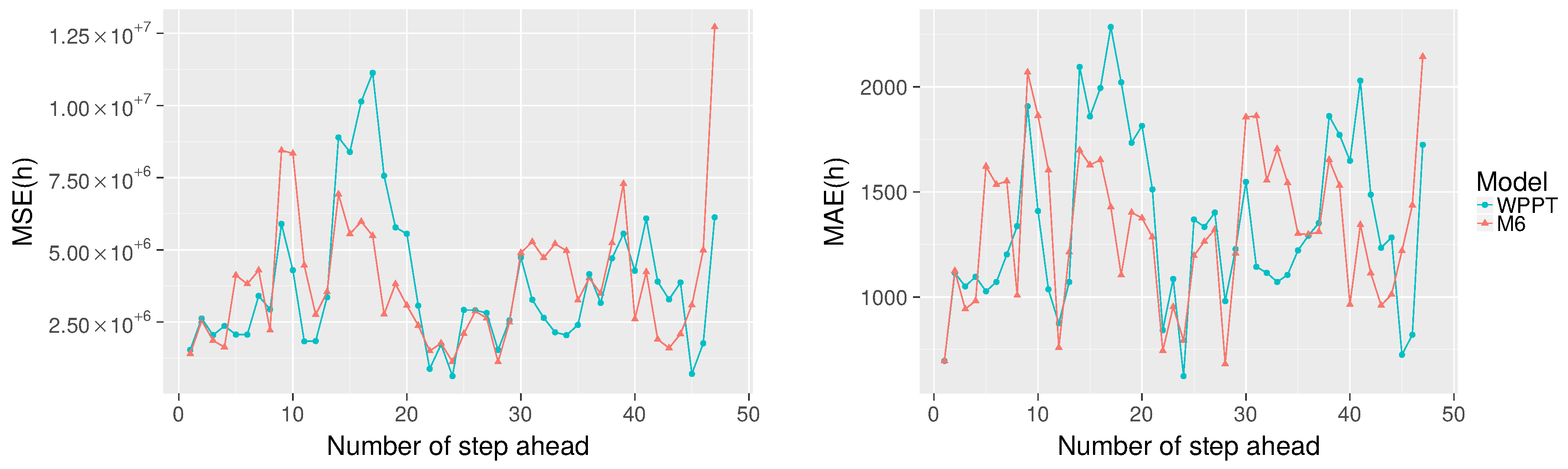
Comparing all algorithms, M7 achieves the best overall MSE; however, M6 reports the best performance in terms of MAE, MAPE and SDE. Given that the M6 model achieves the smallest error in three out of four global metrics, we choose this model to analyze and compare the MSE and MAPE for each step ahead individually using Equations (
18) and (19) respectively against the WPPT forecast.
Just as before, the missing values in the WPPT forecast are not considered in the computed error for M6. In particular,
is discarded because it is not present in the WPPT forecast.
Figure 8 shows MSE(h) on the left and MAE(h) on the right, for each step ahead (from 1–47) averaged over the 10 subseries. It is observed that M6 obtains a lower MSE 51.06% of the time (24 out of 47 predictions) and 57.45% of the time (27 out of 47 predictions) when using MAE. In addition, it is observed that M6 underperforms compared to WPPT until
. However, as
h increases, we can identify time stretches (when
and
) where the proposal outperforms WPPT.
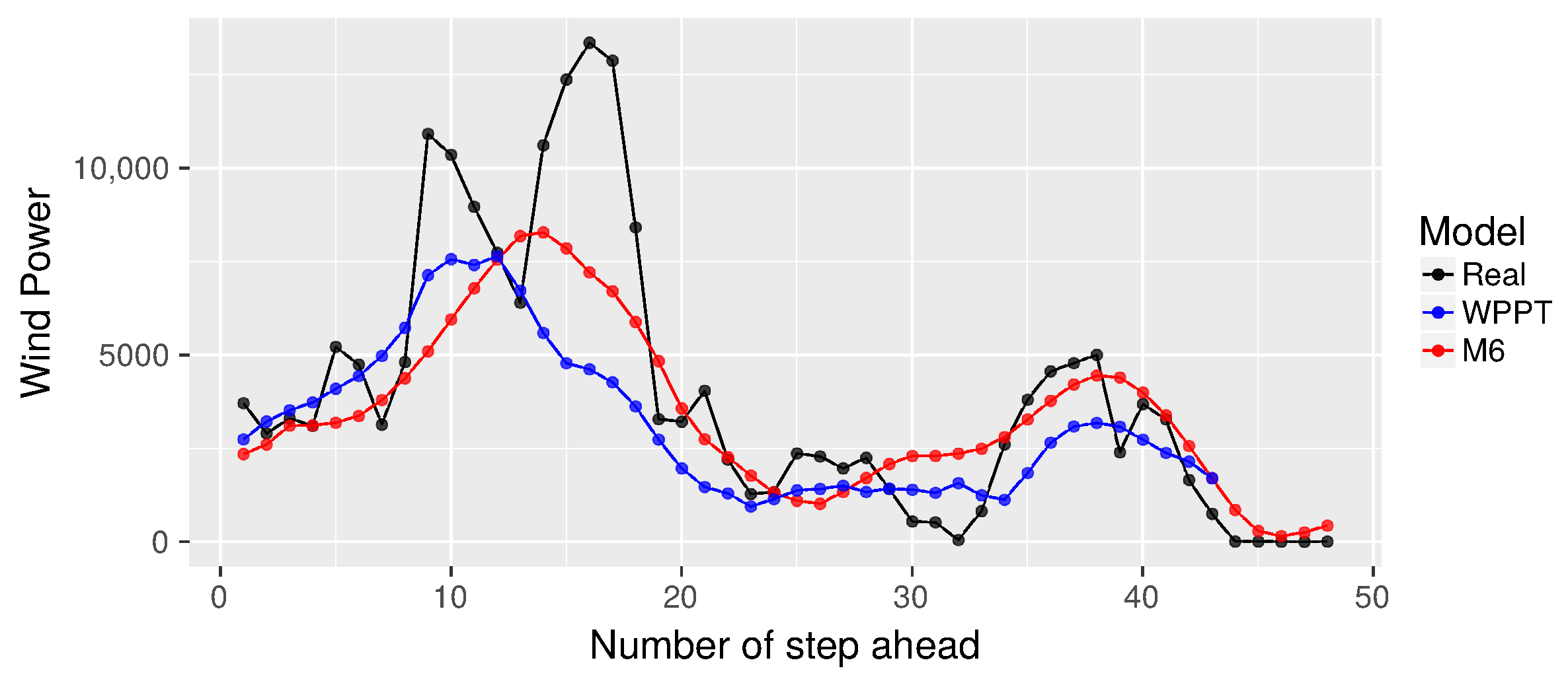
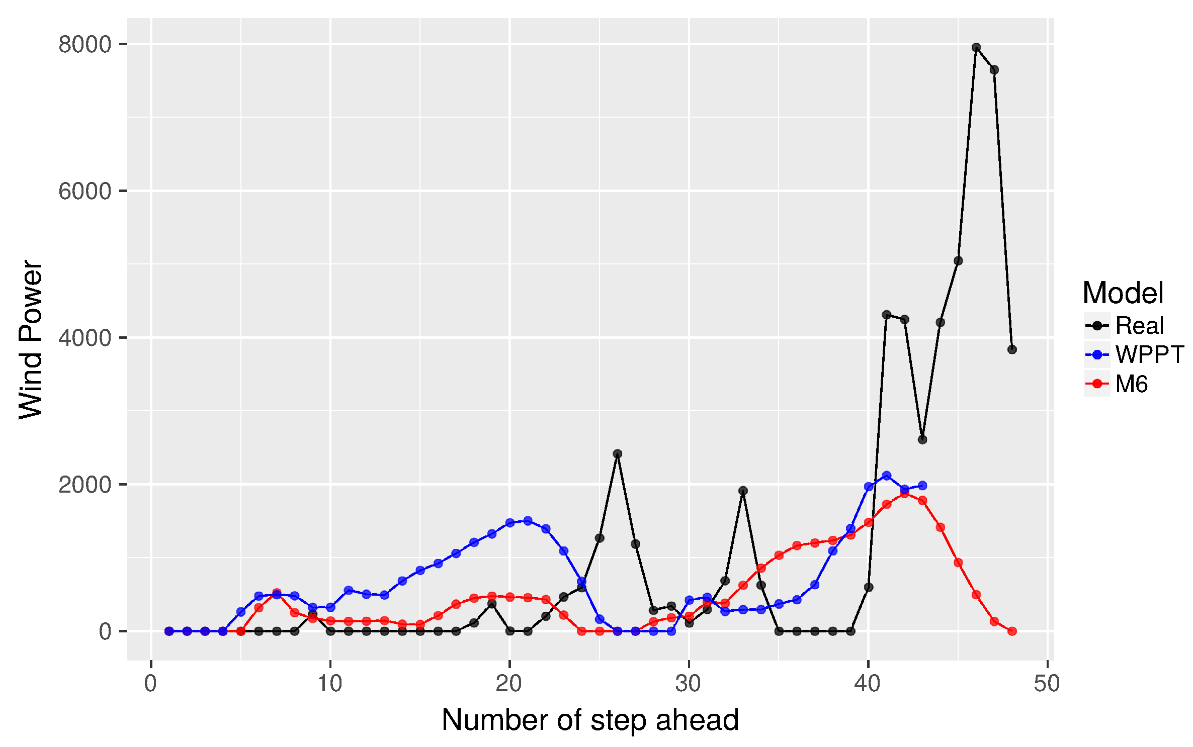
Finally,
Figure 9,
Figure 10 and
Figure 11 show the WPPT and M6 forecasts for subseries
r=1, 5 and 10, respectively. From
Figure 9, we note that the proposal tends to follow the trend of the real curve, omitting the jumps that occur in
and in
. It is also possible to contrast
and
, where the proposal gets better global performance in terms of MSE and MAE. This confirms that the M6 Algorithm tends to mimic the real curve.
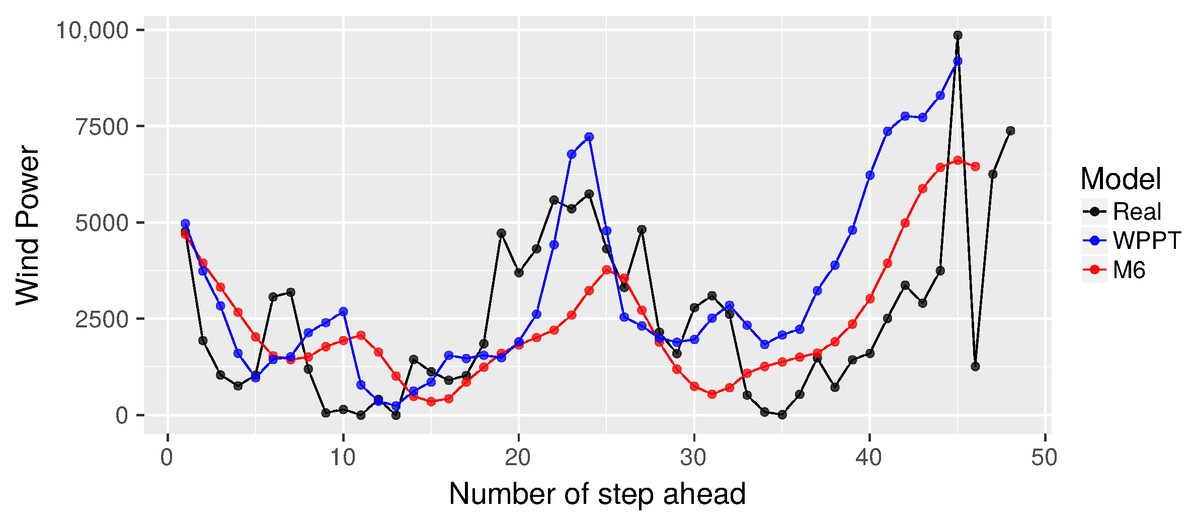
On the other hand, from
Figure 10, it is again confirmed that when
, the proposal exhibits a forecast closer to the real curve. However, when
, there are some differences, where our proposal does not reach the curve’s highest points. This may be due to the cost function used to minimize, which is more restrictive for estimating the median. On the contrary, in
Figure 11, the opposite behavior is observed, that is the proposal achieves a greater similarity in
, but has difficulties in
. In addition, M6 appears more like the real curve in contrast to WPPT from
to
, then tends to present a behavior similar to WPPT.
6. Conclusions
In this paper, a neural network model is presented combining the characteristics of two recurrent neural networks to predict wind power from 1–48 steps forward, modeling meteorological variables and historical wind power. The proposal uses an architecture type ESN of three layers (input-hidden-output), where the hidden units are LSTM blocks. The proposal is trained in a two-stage process: (i) the hidden layer is trained by means of a descending gradient method, using as a target the X input or the Y output, being the first option inspired by the autoencoder approach; (ii) the weights of the output layer are adjusted by means of a quantile regression or ridge regression, following the proposal of a traditional ESN.
The experimental results show that the best overall results in terms of MSE, MAE, MAPE and SDE are obtained when the hidden layer of an LSTM+ESN network is trained as an autoencoder and when adjusting the output layer weights using quantile regression. That is, it is not enough to only make a robust Y estimation (based on the cost function to be minimized) to improve performance; nor is it enough to only model the X input by extracting characteristics. It is necessary to combine these two approaches to achieve better performance.
In addition, when we compare the results with the forecast generated by WPPT, the proposal also achieves a better global performance in all proposed metrics. When analyzing the results of MSE (h) and MAE (h) for each step ahead, the proposal shows time stretches where it achieves the best performance. From the forecast curves, it is observed that the proposal often tries to follow the real trend, and there are time stretches where the proposal is closer to the real curve than the WTTP model.
It is important to remark that this proposal only models wind power from available data, without the need to use power plant information, such as the power curve. Moreover, the evaluated proposal is fed only with current data (lag = 1) and uses only two epochs in the training process: (i) one epoch to train the hidden layer and the output layer sequentially, Lines 6–7 of the Algorithm 3; (ii) and one epoch to perform the “fine tuning” stage, Lines 13–33 of Algorithm 3 using MaxEpochGlobal = 1; making it an efficient machine learning approach. Finally, our proposal trains all the layers of the model, taking advantage of the potential of its architecture in automatically modeling the underlying temporal dependencies of the data.


