Review of Control Techniques for HVAC Systems—Nonlinearity Approaches Based on Fuzzy Cognitive Maps
by
 , and
, and
Farinaz Behrooz
1,2,* ,
,
Norman Mariun
1,2,
Mohammad Hamiruce Marhaban
1,
Mohd Amran Mohd Radzi
1 and
Abdul Rahman Ramli
3 1
Department of Electrical and Electronic Engineering, Faculty of Engineering, University Putra Malaysia, Serdang 43400, Selangor, Malaysia
2
Centre for Advanced Power and Energy Research, Faculty of Engineering, University Putra Malaysia, Serdang 43400, Selangor, Malaysia
3
Department of Computer and Communication Engineering, Faculty of Engineering, University Putra Malaysia, Serdang 43400, Selangor, Malaysia
*
Author to whom correspondence should be addressed.
Energies 2018, 11(3), 495; https://doi.org/10.3390/en11030495
Submission received: 29 November 2017
/
Revised: 1 January 2018
/
Accepted: 9 January 2018
/
Published: 27 February 2018
(This article belongs to the Special Issue Energy Efficient and Smart Cities)
Abstract
:Heating, Ventilating, and Air Conditioning (HVAC) systems are the major energy-consuming devices in buildings. Nowadays, due to the high demand for HVAC system installation in buildings, designing an effective controller in order to decrease the energy consumption of the devices while meeting the thermal comfort demands in buildings are the most important goals of control designers. The purpose of this article is to investigate the different control methods for Heating, Ventilating, and Air Conditioning and Refrigeration (HVAC & R) systems. The advantages and disadvantages of each control method are discussed and finally the Fuzzy Cognitive Map (FCM) method is introduced as a new strategy for HVAC systems. The FCM method is an intelligent and advanced control technique to address the nonlinearity, Multiple-Input and Multiple-Output (MIMO), complexity and coupling effect features of the systems. The significance of this method and improvements by this method are compared with other methods.
1. Introduction
In recent decades, building occupants’ demands for thermal comfort are increasing and hence, the number of HVAC systems has increased correspondingly. Due to the fact these devices account for almost 50% of the total energy usage in buildings [1], improvement of the applied control techniques could be a more efficient way of preventing energy losses by these devices and maintaining thermal comfort at the same time. The HVAC system and specifically the air conditioning system are nonlinear, and complex and in reality are MIMO devices with coupled parameters [2].
Regarding the significant concern of control engineers, which is how to mimic the real condition as closely as possible with the intention of designing systems to be as much as possible applicable, designing advanced control techniques with regards to the features of the system is needed. The features of the HVAC systems are MIMO, time-varying, nonlinear, complex models and coupling effects between parameters [3,4,5]. From the other point of view, the major problems of HVAC systems are variation in system parameters, variable conditions, and interactions between climatic parameters, intense nonlinear factors and uncertainty in the model. Consequently, the systems present significant nonlinear behavior and time-varying characteristics, so linear control techniques cannot offer appropriate performance and stability level solutions, particularly over the wide operating range and when the system’s nonlinearity has a special influence on the system behavior, making the need for nonlinear control essential.
As Afram and Janabi-Sharifi [3] reported, the control law in nonlinear controller design could be derived by using feedback linearization, adaptive control techniques and Lyapunov’s stability theory. In general, more techniques are used like input to state linearization, compensation of static nonlinearities, input to output linearization, sliding mode, relay control, neural network and fuzzy control. The control law is used to drive the nonlinear system toward a stable state while meeting the control objectives. Although the nonlinear control techniques are successful in some nonlinear cases, they need the complex mathematical analysis and identification of stable states for controller design. For instance, the robustness is difficult to guarantee in the case of HVAC systems due to the varying conditions in buildings. Some of the control methods like nonlinear control methods, need the specification of additional parameters, and integration of these additional parameters with HVAC system could be difficult and sometimes impractical, like observers for estimating the thermal and moisture loads. As well, some control methods like nonlinear control do not consider the various constraints on states and controls to reflect the real conditions [6]. In other words, some factors limit the usage of nonlinear control for HVAC systems.
Furthermore, most of the practical systems are MIMO systems in nature [7]. With the purpose of making the system simpler by decoupling the system, the system is considered as a Single-Input and Single-Output (SISO) system. With regards to a SISO system with the aim of controller design [1], the performance of transient control of decoupled feedback loops is naturally reduced. As the coupled parameters are affecting each other, artificially decoupling of them would result the reduced and imperfect control performance. On the other hand, the previous MIMO controllers [2] are based on the system’s linearized models in the neighborhood of the system’s operating point. This means, the system is designed to work around the designed specific operating point and is stable around this designed operating point of the system. Accordingly, the controller is not practical for wide range of operating. As a result, the aim of this review is investigation of the different control methods applied to HVAC systems. The benefits and shortcomings of these control methods are investigated as well.
2. Control Approaches to the HVAC and A/C Systems
Different control approaches are implemented on HVACs which are categorized as classical control, hard control, soft control, fusion control and other control methods [3,6,8]. Also, they could be categorized as traditional, advanced and intelligent controllers [1]. These categories in some parts that overlap. Schematic diagrams of different applied control methods for HVAC systems are shown in Figure 1.
2.1. Traditional or Classical Control Category
Traditional control methods are divided into two subgroups: On/Off control methods and Proportional, Integral and Derivative (PID) control modes. Referring to [1], the conventional control methods are used due to their low initial cost and their simple structure.
The On/Off control mode could be only maximum or zero. This type of controller only has ability to make turn a thermostat, pressure switch and humidistat on or off. Due to the simplicity of this method [9], it is not accurate enough. The quality of this controller is not enough due to its low cost [1,9]. The action of a typical On/Off control method is illustrated in Figure 2.
The other type of traditional control method is Proportional, Integral and Derivative (PID) control which has been utilized in many applications and studies in this field [1,6]. The PID controllers are feedback controllers which work based on the errors of the system (differences between measured values and desired set point values). The term proportional is relevant to the present offset, the term integral is relevant to the past errors accumulation and the term derivative shows the future offset by considering the rate of changes of the process. P and PI controllers are the most used control algorithms. Thermal process dynamics can be considered as slow responding processes in buildings, in which a proportional controller can be used to control the temperature with an acceptable small offset and good stability. These controllers are used for humidity control in buildings as well. The derivative control are combined with (P + I) control to combat the sudden load changes in the system, while keeping the zero offset under steady state conditions. Figure 3 indicates the action of a PID controller. PID controller were used in four levels of supervisory control, maintenance, the controllers to take care of the actuators and local control loops performance, and finally on the level to keep the setting of the controllers based on the model [10]. This structure needs a parameter estimator and control algorithm for self-tuning of the PID controllers by specific references. The Ziegler-Nichols (Z-N) method was used for tuning the PID parameters to investigate the influences of the disturbances on the settling time and overshoot by Tashtoush et al. [11] which is applicable in small normalized time delays and with normalized gain could be usable for further PID tuning. In addition, the Dounis et al. [12] applied a PID controller based on Z-N on a dynamic model of a HVAC system to reduce disturbances, reduce the energy usage of the system and improvement of indoor comfort.
Due to the linearity of PID controllers, using them in nonlinear systems like HVAC or A/C systems causes variable performance of the system. For instance, in the case of temperature control, the overshoot of the system could be corrected gradually. By tuning the PID to be over damped and overshoot reduction and prevention which may results in reduced performance of the system and an increase in the settling time.
Despite the fact that, the conventional controllers are widely used and have acceptable functions, in consequence of high maintenance and low efficiency, it provides evidence of high cost. As Perera et al. [9] reported, the traditional control methods can be used for controlling the systems with certain limitations. These control methods can be easily tuned for SISO systems but tuning of these methods for MIMO systems are not easy and sometimes are impossible [3]. Table 1 shows the advantages and disadvantages of classical or traditional control techniques.
2.2. Hard Control Category
The hard control strategies consist of [6]:
- Optimal control method,
- Robust or H∞ control method,
- Adaptive control method,
- Non-linear control method, and
- Model Predictive Control (MPC).
2.2.1. Optimal Control
According to the nature of the optimal controllers regarding human comfort and energy savings, they are widely used in this area. The purposes of using optimal control in HVAC systems are mostly minimizing the energy usage and control effort of the systems and maximizing the thermal comfort [3]. Referring to Mirinejad et al. [1], the primary goals of HVAC systems, which are mostly occupant’s thermal comfort and energy efficiency are sacrificed. By applying optimal control methods which have energy saving potential, a minimum amount of energy is used to achieve the desired comfort temperature and humidity.
Optimal controls or supervisory controls [17] are always pursuing the minimization or maximization of a real function by systematically selecting values of parameters or variables within acceptable ranges. In other words, entirely monitoring the system and completely controlling the local subsystems can be done by optimal control [18]. Therefore, in the case of controlling HVAC systems, optimal control or supervisory control goals seeking the least possible input energy and operating cost to provide a healthy atmosphere and thermal comfort, take into consideration the total outdoor and indoor changing conditions along with the properties of the HVAC systems. By optimal controls all characteristics of the system level and interactions between variables could be easily considered. By knowing and utilizing the system’s characteristics and interactions knowledge, the objective function or cost function could be reached. As a result the system response will be improved and operating cost will be reduced [17]. Requirements for optimal control problem’s formulation are as follows:
- Controlling the system based on mathematical model to arrive at optimal objectives,
- Specifying the performance index,
- Requirement to all boundary conditions on states, and constraints to be satisfied by states and controls, and
The optimal control strategy for obtaining the twofold objective of minimizing a cost function and maximization performance could rely on different models of the system such as white, grey or black box models [17]. The mathematical model is utilized to design the optimal control strategies for controlling the building’s heating [20,21,22,23]. The grey box model for optimal control method was used by Berthou et al. [24]. The data from one floor of the elementary school building are measured for identifying a grey box model. Due to their quick run-time and liability to constraints, the grey box models are well adapted to perform optimization [24].
As Ho [25] and Pannocchia and Wright [26] reported, although optimal controllers were successfully used in the aerospace industry like for the Apollo moon landing and global positioning system (GPS) between 1950 to 1960 and also in the HVAC field between 1989 to 2010, their weak point is their inherent complexity. If the problem has no particular structure like the linear, unconstrained models which constitute the classic or typical Linear Quadratic (LQ) regulator, evaluating and applying online the optimal feedback control represents an intimidating challenge.
The Linear Quadratic Gaussian (LQG) controller was applied on a linearized model of the MIMO Direct Expansion (DX) A/C system by Qi and Shiming [27]. This method controls the humidity and temperature by varying the supply fan speed and compressor speed. Disturbance rejection, set point tracking and superheat control’s improvement were reported by Qi and Deng [28]. In other words, the MIMO controller are able to control the indoor air humidity and temperature together with acceptable control accuracy and sensitivity in disturbance rejection and set point tracking. This method applied a linear model of the system and it is applicable only for a specific operating point. As a result, it cannot be implemented for a wider operating range.
Optimal Model-Based Controller is used in HVAC Systems. The optimal control policy are respected by the system during the perfect set point tracking for the inlet air temperature, but the linearized model from the derived nonlinear model was used for designing the controllers [29]. Model-based hierarchical optimal controller has been done by linearizing the model nearby the system operating point and also a Linear Quadratic Regulator (LQR) supervisory controller are used for selecting the optimal set-points for the lower level PID controllers [30].
MATLAB/Simulink response optimizer, Input/output feedback linearization, and nonlinear programming are used to design Non-Linear Optimal Controller for HVAC systems by Dong [31]. A great energy saving potential has been achieved by using an optimal controller, which contributes to the development of energy efficient and sustainable buildings. It requires the specification of additional parameters, which could be difficult and impractical for integration in HVAC systems, and is a disadvantage of this controller. One of the important disadvantages of the optimal control strategies is the need for an appropriate model of the system for designing the controller [32,33,34,35,36,37,38,39,40,41]. Table 2 indicates advantages and disadvantages of the optimal control methods.
According to Naidu and Rieger [6], in the matter of system nonlinearity and model uncertainty the robust control solution could be applicable. As a result of the attractive features of the robust control regarding uncertainty in model parameters, measured, unmeasured or external disturbances, it was successfully applied to cancel the disturbances in set point tracking. Besides, prior uncertain inputs knowledge is not required. Although this method is advantageous in disturbance rejection and set point tracking, it is not a suitable choice under weather conditions with drastic changes [15]. As Venkatesh and Sundaram [15] reported, a nonlinear robust control method which was used by Soldatos et al. [42] in livestock building to control the humidity and temperature by considering the bounded and unknown errors could also be used for air conditioning systems. This method was very successful in the case of external disturbance rejection and set point tracking. Since the combination of feed forward and feedback control are implemented in the nonlinear robust controller, it is able to cancel the unknown and external disturbances [15].
MIMO robust control was used for HVAC systems by Anderson et al. [43]. The application of robust MIMO controls to an HVAC system offers a better improvement in the performance of the HVAC systems. The experimental results show that compared to the PI controller, the MIMO robust controller offers slightly improved disturbance rejection. Table 3 illustrates the merits and demerits of the robust control techniques.
2.2.2. Adaptive Control
Due to the HVAC systems’ characteristics like nonlinearity, complexity and time varying nature, the adaptive control strategy offers different solutions for nonlinear models and slow time varying parameters and uncertainty [6]. Based on work by Landau et al. [44] and Perera et al. [9], the adaptive control methods could be considered as a specific kind of nonlinear control method for systems or processes in which the dynamics change during normal operating conditions due to stochastic disturbances. During the operation of the system, online information of the system and process has been obtained by a closed loop for control issues. By using the adaptive control methods the desired set points for control system performance can be achieved and maintained. In comparison with the conventional methods, the adaptive methods by using the inputs, outputs, the states and the identified disturbances can measure a specific performance index for controlling the system. Then, by comparing the measured performance index (PI) with the reference PI’s, we can adjust the parameters of the controller by an adaptation mechanism for maintaining the required performance index of the control process. Therefore, adaptive methods are feedback types with two feedbacks, one for handling the process signal variations, the other for handling the process parameters changes to make the control adaptive. Figure 4 depicts a schematic of the adaptive control method.
As Song et al. [16] reported, for designing adaptive control strategies, a model of the system is necessary. As a result of adaptive controller’s ability to self-regulate, they are applied in several types of buildings in different climate conditions. Especially the adaptive fuzzy controllers are the most capable among the other types of adaptive control systems used for buildings [45]. The other solution could be using the parameter estimation methods like Recursive Least-Squares estimation (RLS) [9,46].
Novel adaptive energy-efficient controllers based on nonlinear adaptive back-stepping control algorithms were used for HVAC systems by Hongli et al. [47]. In this method the Lyapunov stability is realized. Energy efficiency of HVAC energy management system is achieved so it has been implemented in the intelligent building energy field. Difficulty in finding Lyapunov stability and the need for a bilinear observer are disadvantages of this method. The advantages and disadvantages of adaptive control technique are listed in Table 4.
2.2.3. Nonlinear Control
As HVAC systems present significant time-varying and nonlinear behavior, linear control techniques cannot offer sufficient performance and stability level solutions, especially over a wide operating range and when the nonlinearity of the system has a beneficial and special effect on the system behavior like in an air conditioning system. Then the nonlinear control technique is required. As HVAC systems are time varying systems, complex and nonlinear, the nonlinear control approaches give different solutions than nonlinear models and slow time varying parameters and uncertainty [6], but the nonlinear control methods could be applied for restricted regions [15]. Since the purpose of this paper is focusing on nonlinear control methods, a comprehensive review on nonlinear control techniques applied for HVAC systems is provided in the following sections.
As Afram and Janabi-Sharifi [3] reported, in the case of HVAC systems the control law in nonlinear controller design could be derived by using the adaptive control techniques, Lyapunov’s stability theory and feedback linearization. In general, more techniques are used like input to state linearization, compensation of static nonlinearities, input to output linearization, sliding mode, relay control, neural network and fuzzy control. The control law is used to drive the nonlinear system toward a stable state while achieving the control objectives. As [3] reported, although nonlinear control techniques are successful in the case of HVAC systems, they need the identification of stable states and complex mathematical analysis for controller design. Generally, in the case of applying the hard control category in HVAC systems, the robustness is difficult to guarantee, due to the varying conditions encountered in buildings. Most of the controllers in the hard control category which are nonlinear require the specification of additional parameters, which could be difficult and impractical for integration in HVAC systems like observers. Besides, most of the hard control category methods so not take into consideration the various constraints on states and controls to reflect real situations [6].
In the case of HVAC systems, the applied nonlinear control methods are limited. According to [48], feedback linearization and gain scheduling methods are separately applied to a nonlinear, MIMO model of an air-handling unit (AHU). The cold water and air flow rates are used to obtain desired tracking objectives of indoor humidity ratio and temperature of MIMO model. Applying the feedback linearization controller causes quicker time responses in humidity ratio and temperature tracking, but with more overshoots. Specially in tracking the ramp sections of desired set-paths for humidity ratio, more overshoots can be seen in the results.
Applying the gain scheduling controller leads into less energy usage by AHU. Less variation of cold water and air flow rates are needed for obtaining tracking objectives when the gain scheduled-based controller is used [48]. The gain scheduling control design’s disadvantageous are need for the identification of linear regions and design of switching logic between regions, and the manual tuning of multiple PID controllers in these regions can be challenging.
Thosar et al. [49] used a feedback linearization method on a laboratory-scale plant of a Variable Air Volume Air-Conditioning (VAVAC) model. Compared with the PI controller, it has great performance in the case of thermal comfort and energy optimization.
In order to describe the humidity and temperature dynamics of the single-zone VAV HVAC&R system, a bilinear model was used by Semsar-Kazerooni et al. [50]. By considering measurable disturbances (heat and moisture loads), the back-stepping controller was designed for the feedback-linearized model. Also a stable observer was designed for non-measurable disturbances backed by simulation results for optimal energy usage. Simulation results show a closed-loop system with quick tracking response, smooth response with high disturbance decoupling and offset-free and optimal energy usage in existence of time-varying loads. Difficulty in finding a Lyapunov function and the use of all state which leads to the need for nonlinear observers, are the disadvantages of this method. In other words, this work involves complex mathematic analysis and integration of different control methods together for controlling the system like decoupling and linearization the model to find some required parameters then applying the other method to transfer the model to the nonlinear form. As a result, due to the complexity of system and model uncertainty, a simple control algorithm with simple mathematics is required. Also, integration of nonlinear observers with HVAC makes this mathematic process more difficult. The advantages and disadvantages of nonlinear control methods are provided in Table 5.
Overview on Different Possible Control Methods for Non-Linear Control Systems
Since there is no general nonlinear control theory, many techniques have been developed. Therefore, the different methods listed as follows with its advantages and disadvantages [51]. Table 6 indicates the advantages and disadvantages of different nonlinear control methods.
Briefly, some of the factors that limit the usage of nonlinear control on HVAC systems are as follows [51]:
- Difficulty in finding the Lyapunov functions,
- Complexity in integration of nonlinear observer with HVAC,
- Sensitivity to parameter variation,
- Limited operating range in state feedback,
- Proof of stability,
- Need for measuring all state variables or additional measurement,
- Possibility only on stable processes, and
- It is necessary that state variables to be all measurable, otherwise, a nonlinear observer is required.
In the case of HVAC systems, the applied nonlinear control methods are limited. Based on Moradi et al.’s [48] work, feedback linearization and gain scheduling methods are separately applied to a nonlinear, MIMO dynamic model of AHU. There are two disadvantages of the feedback linearization method:
- Additional measurement is needed, and
- More overshoots are produced.
By using the gain scheduling controller, the energy usage of AHU is decreased. A reduced amount of variation of cold water and air flow rates are used in order to achieve the tracking objectives by using the gain scheduled-based controller [48]. Referring to Afram and Janabi-Sharifi [3], for gain scheduling control design, it is imperative that between regions, the design of switching logic and linear regions to be identified., and the manual tuning of multiple PID controllers in these regions can be quite cumbersome. In general, in the gain scheduling control method the disadvantages are as follows:
- Finding dependency between scheduled variables and parameters values certain engineering exertion is demanded,
- Slow operating point’s alternation resulted in the controlled system nonlinear behavior, and
- A problem could be raised due to the proof for stability.
For obtaining the control objectives and energy usage by the system, an observer was designed in the feedback control system for estimating the state variables of the system and also the regulator was designed for disturbance rejection. The tracking objectives of the system were obtained and compared by designing nonlinear control methods of feedback linearization and gain scheduling separately on the system. Desired set points of indoor temperature and humidity ratio were tracked with changing the flow of the cold water and air. The feedback linearization method has a faster time response but contain overshoots. The cold water variation for both controllers are almost similar, but for feedback linearization controller used more air flow rate variation in compare with the gain scheduling controller. The gain scheduling control method has less changes of cold water and air which results in decreased energy consumption of the AHU.
A model of Variable Air Volume of Air Conditioning (VAVAC) by Thosar et al. [49] was utilized a feedback linearization technique for designing the nonlinear control systems. It was simulated with a laboratory-scale plant. Besides, for explaining both humidity and temperature dynamics, the single-zone VAV HVAC & R was accounted by Semsar-Kazerooni et al. [50] bilinear model. Considering moisture and heat loads as measurable disturbance, a back-step controller was designed for the feedback linearized model. For optimal energy usage, a stable observer was designed for non-measurable disturbance supported by results of simulation. Disadvantageous of back stepping technique are as follows:
- Requiring a nonlinear observer, unless all state variables are measurable,
- Having measurable state variables,
- Complicated task in identifying a Lyapunov function, and
- Sensitive to parameter variation.
Moreover, Hodgson [52] and Pasgianos et al. [53] used the adaptive control technique to derive a control law based on steady state. Although a wider operating range could be possible by this method, the disadvantages of adaptive techniques are as follows:
- The lead often to nonlinear observer problems,
- the adaptation loop is essential to be slower than the loop of control, and
- Stability proof is complicated, specifically in situation of changing process parameters.
The previous applied nonlinear techniques are involved with identification of the stable state, complex mathematical analysis and linearization around an operating point. It means that these control techniques use difficult and complex mathematics. Also, the uncertainty of the HVAC system models makes the process of designing a suitable controller very difficult and by linearizing the model, the operating range will be limited.
2.2.4. Model Predictive Control (MPC)
For predicting the system’s future states, a model of the system is required in predictive control methods. Due to the benefits of the predictive control methods, energy saving and cost effectiveness are achieved by generating a suitable control vector in the existence of constraints and disturbances [54,55,56,57,58,59]. Regarding the HVAC characteristics, the predictive methods provide a practical solution. For instance, the HVAC systems are internally time-varying, and slow moving with time delays, external disturbances act on the system, high energy consuming, operating condition range of the system is wide, and actuators exhibit rate and range limit constraints. The MPC method is able to handle many of the aforementioned problems.
MPC is a kind of multivariable control technique which is based on a prediction model. It means the past information of the system and future inputs are utilized for prediction of the future output of the system. The MPC method is widely used in process control applications. In order to minimize the cost function, a system model is used to generate a proper control vector. In each sampling the first element of the calculated control vector is used as a system input, and the remainder are discarded. This process is repeated each time for the next step. The cost function could be a tracking error, energy cost, power consumption, demand cost, control effort or other factors. The limitations and rates of the actuators, manipulated variables and controlled variables can impose constraints like supply air flow rate, maximum and minimum of the zone temperature and damper speed limits. Disturbances such as occupant activities, weather, and equipment use which are modelled as well could be considered, so their predicted influence on the system is calculated in the control vector. As a result, this controller is robust to both time-varying system parameters and disturbances and it is able to regulate the process within the given bounds. Any type of the model could be used in designing the MPC like black box, grey box and white box [59].
In the dynamic first order models, finding the first principles model of the system could make the process very time consuming due to the complexity of the building structure. On the contrary, data driven methods like grey and black box are fit to the nonlinear and linear mathematical model of the system for measuring the system’s data, but for more accuracy of the data driven models, quality measured data are required. Therefore, all the measured data should be more accurate, based on the process need for a suitable sampling frequency and low noise or disturbances. The high quality models which are more accurate increase the complexity of the model. The low quality models are not suitable for energy saving goals, hence models with less complexity are required to achieve computational simplicity and reasonable accuracy [9]. Nevertheless, implementation of the MPC is advantageous in the field of HVAC systems because of its simplicity in developing the control strategy in the case of uncertainty.
Xu et al. [60] utilized the Generalized Predictive Control (GPC) method for tuning the parameters of PID controller. Besides, for decoupling HVAC & R systems together with parameter identification, Xu and Li [61] employed GPC method. GPC method is in less demand of computation comparing to the coupled system. Ferhatbegovi’c et al. [62] employed a predictive control concept for a solar powered HVAC system. The basic of the controller is on the components of dynamic HVAC models validated according to the measurements conducted on a real system of HVAC. The perfect operation of MPC approach is demonstrated by applying the information of weather forecast where proper operation is shown by the MPC concept, even if the weather forecast shows incorrect information. Whenever the predicted information is incorrect, the receding horizon strategy of MPC concept exactly used for this circumstances. The MPC control structure was applied on the real solar powered HVAC system by Ferhatbegovi’c et al. [62]. The solar pump and the storage pump in the MIMO MPC controller were used as actuators. The aim of the controller is controlling the differences of the inlet temperature to the heat exchanger ( = − ) and the outlet temperature to the heat exchanger (Δ = − ) for working around the defined operating point. The turning on and off the pumps are based on the weather data. The solar radiation are using as a decision value in order to switching the pumps on and off condition. The disturbances of the systems are the ambient temperature (Tamb) and the global solar radiation (Gt). The other disturbance of the system is which is the effect of the tapped water on the storage tank as a result of the heat pump system and the thermal heating and cooling systems activated in the building. The manipulating variables are and which are the activation of the storage and solar pumps. The optimal input trajectories in each time instant are calculated based on the control horizon Nc. Also, the control inputs for time instants k ∈ [Nc+1, Np] are considered constant. The weather forecast information like ambient temperature and solar radiation are used to analyze the predictive control concept. The objectives of this method are the optimal using of the renewable energy source like sun light and reducing the energy usage of the pumps. The non-correct weather data (nok) does not remarkable effect on the control performance. The control inputs and which at time instant k ≈ 2.5 h, by detecting negligible radiation of solar, causes both pumps to turn off. Table 7 reveals the advantages and disadvantages of model predictive control methods.
2.3. Soft Control Category or Intelligent Control Category
Regarding the complexity, nonlinearity and MIMO structure of HVAC systems, identifying an appropriate mathematical model for them could be a challenging task. Due to lots of disturbances, time delays, contingencies and vagueness about thermal comfort, make finding a proper mathematical model for the system much more difficult [69]. According to the structure of the intelligent control methods, a model of the system is not required for designing the controller and it only depends on the human’s thermal comfort feeling. Accordingly, the intelligent control methods avoid the mathematical model development for different building structures. As a result, intelligent controller methods are used widely in the case of HVAC systems [69]. These methods can directly be applied for HVAC systems and they can be used as well to improve the traditional controller methods [9]. The soft control or intelligent control strategies consist of:
- Neural networks control method (NNs),
- Fuzzy logic control method (FL),
- Genetic algorithms method (GAs), and
- Other evolutionary methods [8].
2.3.1. Artificial Neural Network (ANN)
The inspiration of artificial neural network (ANN) is based on the nervous system, human brain and learning process of neurons. The ANN method involves with a set of interconnected neurons divided into input, output and hidden layers. The outputs of the system are calculated based on the inputs to the system and network weights and the transfer function of the network. Due to the adaptability of this method by its self-tuning process, the ANN method is widely applied for HVAC systems. The training of the ANN is achieved by the weight coefficient regulation to minimize the cost function. The ANN-based controllers do not need an identification model of the system [16].
Based on the structure of a neural network which is the generic method to represent or map the relationships between the inputs and the outputs, patterns of nonlinear functions and also pattern the data through layers of an interrelated grouping of artificial neurons that is called artificial neural networks or simply neural networks [70]. It could be an attractive choice to control and identification of nonlinear systems like HVAC systems. As Daponte and Grimaldi [71] reported, the architecture or simply the algorithm of this method is based on a neurobiological system. It means this method could be considered as a black box with great predictive capacity for the models. It is very useful, especially in the case of unknown models or when the mathematical model is not available or when all of the characters are described in unidentified conditions and able to train the ANN [72]. Referring to Wu and Li [73], this method could be an interesting choice in the case of controlling nonlinear systems as a result of its robustness, ability to map arbitrary nonlinear functions, great capacity in model prediction and nonlinear recognition when a mathematical model is not accessible. Based on Mirinejad et al. [1], most common neural network controllers in HVAC systems are based on a predictive controller which is extracted from the construction of a system model used in the controller regulating in the nonlinear systems or direct controller which is very simple and output feedback controller with no need for training.
Although the neural networks have ability to deal with both nonlinear and linear systems, however, they are mostly applied in nonlinear systems [74]. Even though the neural networks have more profitable advantages like lots of tasks could be done by neural networks which cannot be performed by linear programs, they also keep continuing the process with no problem when a failure take place because of its parallel nature. But this method has some disadvantages which cause a decrease in the efficiency and performance of this method such as the operation of a neural network requires training and takes a long time to process a large neural network which means this model is far from real time control. The NN controller was applied in the outer loops of the AHU of the HVAC & R system by Guo et al. [75]. This method created an adaptive and robust system by applying the simultaneous perturbation stochastic approximation training on multi-layer NN to guarantee the whole control system’s stability. The performance of AHU in controlling the temperature was improved for temperature set-point tracking and disturbances rejection of the chilled water flow rate. The ANN control method’s advantages and disadvantages are shown in Table 8.
2.3.2. Fuzzy Logic (FL)
Fuzzy logic is fundamentally a methodology which is based on human reasoning and a linguistic model by applying uncomplicated mathematics in the case of nonlinear, complex and integrated systems. Membership functions and rules are used to form the reasoning and human knowledge in this methodology. Compared to conventional controllers, this method does not require a mathematical model of the system and it is grounded by human knowledge about the system’s behaviour [1].
Fuzzy logic control methods consist of three steps as fuzzification, fuzzy inference and defuzzification. The fuzzification process transfers the crisp values of the inputs to the fuzzy values. Suitable membership functions are applied like Gaussian distribution triangular, bell functions, trapezoidal, and sigmoidal functions to map the input values to a degree of membership in the range of [0,1]. The next step is using a fuzzy inference system to map fuzzy values to different fuzzy values by applying the fuzzy IF-THEN rules and logical operations. The fuzzy inference systems are divided into two types, Mamdani and Sugeno. The Mamdani type is used for all types of the systems while the Sugeno type is mainly used for dynamic nonlinear systems. The aggregation of the linguistic output values from previous step are used for defuzzification process. Finally, the defuzzification process produces a single crisp value as an output.
Although this method has a good record in the case of HVAC systems, there are some shortcomings like more fuzzy grades are required to achieve higher accuracy in the system [76], and cause an exponential increase in the rules and run time of the system [77], and feedback receiving for implementing a learning strategy could not easily be applied [78]. As Naidu and Rieger [8] reported, assigning the required set of membership function in fuzzy logic control strategy regarding to tuning and optimizing the data base and pre-defined rule base would be very time consuming and difficult, specifically for optimization of energy consumption and high thermal comfort as multi-objective functions. There are pure fuzzy logic models [79], and semi-fuzzy systems [80], and incorporated PID and Proportional–derivative (PD) controllers into the rule-based body of the system [81]. A similar principle is applied to all the types of fuzzy controllers, where input variables are usually entered into a block of expert-defined rules which acts as the inference mechanism and outputs are provided based on the existing rules in the inference mechanism and the implemented defuzzification method. Accordingly, there are output controls to be applied to thermal, light or other actuators. The input and output variables are defined with respect to the application for which the system has to be designed. For example, in a naturally ventilated building for summer conditions [79], the outside wind velocity, and direction, and the outside and inside temperatures can be taken as input variables. In such a system, the control output is the degree of openness of a window louvre. In this system two fuzzy controller based on the IF-THEN rules or using different membership function were applied. The comparison of the results shows that the controller with more IF-THEN rules is more responsive for changing the outside conditions. It means that this controller is capable in order to adjusting the louvre opening positions when the indoor and outdoor conditions change. Some semi-fuzzy controllers are applied by Kolokosta et al. [80] which were designed for adjusting and maintaining the air quality, visual and thermal comfort of occupants in the buildings and reducing the energy usage at the same time. The designed methods are fuzzy PID, fuzzy PD and adaptive fuzzy PD which are compered based on required energy and response of the controlled variables. Comparison shows that energy usage and variables responses were improved by adaptive fuzzy PD by cancelation of overshoots and oscillations. Also, the non-adaptive fuzzy PD controller is appropriate for indoor visual comfort.
System inputs are physical variables that are used to completely determine the state of the system. In fuzzy control, the inputs are fed to the controller using fuzzy grades of membership functions. Zemmouri and Schiller [82] developed a system for interior daylight control. In this system, one of the input membership functions is associated with the opening of the facade of the building. Such a function is used to assign four fuzzy grades to the input variable of openness including: closed, medium, open and very open. There are another two input variables whose membership functions get 3 and 4 fuzzy grades respectively. Therefore, the number of required rules for describing the fuzzy rule-based controller is 4 × 3 × 4 = 48. Advantages and disadvantages of FL methods are listed in Table 9.
2.3.3. Genetic Algorithm (GA)
According to Naidu and Rieger [8], the biological evolution theory is the base of genetic algorithm by considering mutation, crossover and survival of the well-matched, especially in multi- objectives function optimization. In other words, this method has a different approach to the optimization intentions without concerning the mathematical model which is a global non-derivative or derivative-free technique, but this method is not always appropriate in the case of real-time HVAC applications.
The genetic algorithm is mostly used for automatic tuning or learning of the components in fuzzy systems which is called Genetic Fuzzy Systems (GFSs). By using the genetic algorithm (GA) the best or optimum solution will be found among the other solutions. Thus, GAs are used as a solution to optimization problems for designing automatic fuzzy controllers [69].
Tuning by a genetic algorithm which is called the Genetic Tuning Method is used for optimization of fuzzy systems’ performance. Actually, the tuning process of fuzzy logic control (FLC) is applied to optimization of both given membership functions (MFs) and input-output scaling gains (SGs). The other method is an automatic process for producing the knowledge base (KB) in FSs which is named Genetic Learning. By applying the Genetic Learning method all rule base (RB), membership functions (MFs), or both, are generated regardless of previous knowledge about one of them or both of them. Therefore, the Genetic Learning is a more difficult task due to the need to generate RB for fuzzy systems in comparison with Genetic Tuning that optimizes the performance of a FS that already operates at least almost correctly [69].
For purposes of thermal comfort and energy saving the GA method has been applied for smartly tuning the FLC in HVAC systems by Alcalá et al. [83]. Although the FLC method is beneficial for applying the linguistic rules in expert knowledge and controlling HVAC systems, collecting the suitable expert knowledge for HVAC control problems is difficult. The initial KB are used by human expert experiences and knowledge of control engineering which consequently are tuned automatically by GA as an automatic tuning technique. The fewer number of rules in expert knowledge systems make the required control process for partitioning the controller possible. As a result, it makes the automatic tuning process simpler due to the fact it affects a small number of rules by modifying the parameters. For tuning the parameters of KB control by developing the GA method, two limitations affecting the design as follows:
- Parameter evaluation could be constructed based on the multiple objectives evaluation like thermal comfort or energy consumption that would force choosing between different criteria’s optimization, and
- Simulation is the initial approach to knowing the controller’s accuracy that commonly takes a long run time, therefore fast convergence is needed for selected tuning algorithms.
To overcome these restrictions the application of objective steady-state GA, weighting method, and reduction of the population size could be beneficial. In the objective weighting method the combination of multiple objective functions is used as one comprehensive objective function through a vector of weights. In the steady-state GA method by selection of the two best population individuals and combination of them two offspring is obtained. By this approach the restrictions and convergence are improved and the number of evaluations simultaneously are decreased [69]. Table 10 shows the merits and demerits of GA control methods.
2.4. Hybrid Control Category
As is obvious, hybrid or fusion control methods are combinations of a soft and hard control or two soft control methods. A better performance can be obtained by using hybrid methods in comparison with using each control techniques alone [8]. Figure 5 describes the schematic of the principle of hybrid control methods.
Advanced controllers with auto tuning strategies are very applicable on both Single-Input and Single-Output (SISO) and MIMO systems in which decoupling of the MIMO systems are required [84,85]. As Mirinejad et al. [1] reported, this procedure is difficult, expensive and time consuming. It is divided into two types: Model-based and Empirical rule-based algorithms. When the parameters are related to a transfer function model, it is referred to as Model-based and when they are identified by heuristic rules, it is referred to as Empirical rule-based. The Self-Tuning Control (STC) is more advantageous, especially in the case of PID controllers, but model identification as an initial step and model parameter identification in real time mode are required. As the HVAC systems are known to be complicated and nonlinear systems with disturbances, the model of the system could not be well identified or it means the model is uncertain. As Rehrl et al. [86] reported, applying a standard simple controller like PI to control the room temperature, as a result of oscillating periodically around a desired value has a poor performance. Moreover, the adaptive PI controller was implemented with exponentially forgetting recursive least square (RLS), dead time model and first-order match model with automatic controller parameters adjusting on HVAC systems [87]. Compared with H∞ adaptive PI, the mentioned controller shows better performance. In comparison, the self-tuning PI controller with applying integral of time and absolute error (ITAE) by RLS in z domain model with a Smith predictor for time delay reduction indicates greater performance [88].
Addressing the weak point of fuzzy logic methods to produce the optimal fuzzy rules and identify the membership functions for more efficient control process, a combination of fuzzy logic and neural network methods which is known as the adaptive neuro fuzzy inference system (ANFIS) could overcome these problems. The ANFIS base control has been applied by Soyguder and Alli [89] to more accurate prediction and control of HVAC systems by different membership functions. The fuzzy sets were used to damper the gap rates. By this method the steady state error and settling time are reduced in comparison with conventional techniques. Increasing the membership function for more accuracy in this system could cause an increase in the run time of the system and it is far from real time control. This controller was not tested in real time and only the simulation results are available.
The Neuro-Fuzzy control methods can help develop optimal fuzzy rules and in determining the membership function parameters but these methods can use a limited number of input variables. All in all the hybrid methods which are combinations of soft controls or soft control methods with hard control methods are able to solve the problems that the individual methods may not solve, but for soft control methods a large quantity of data are required in order to train and tune the hard controllers and advanced controllers are difficult to implement [9].
The hybrid intelligent, MIMO controller was utilized on DX A/C system based on combination of soft computing methodology of Fuzzy Cognitive Map (FCM) and Generalized Predictive Control (GPC) method Behrooz et al. [90,91]. By implementing the GPC-FCM method in order to control the DX A/C, all the problems of the systems were considered and solved. The main contribution of this work was to offer a new approach as an intelligent MIMO nonlinear controller for DX A/C which could be expanded to the HVAC. This new designed controller were applied easily and efficiently. The effectiveness of the proposed control system was evaluated in a simulation environment. With the purpose of full controlling of DX A/C system, this hybrid controller was used. This hybrid control method is capable to consider the MIMO, nonlinearity and coupling effect properties of DX A/C system. Due to the specific structure of FCM for solving the problems, the inputs and outputs of the system can be considered together as a MIMO structure controller. Correspondingly, the coupling effect among the parameters could be considered by causal relationship of required concepts. Last of all, the outcomes has been utilized to the nonlinear model of the system. Artificial decoupling of the parameters is omitted in the FCM structure. In consequence, increased control performance and improved sensitivity and accuracy of the controller are achieved. The proposed control system benefits from the graph structure of the FCM with simple mathematics, which avoids the complex mathematical analysis one normally needs to deal with when designing a control system for a MIMO system with complex nonlinearities [90].
3. Introduction and Description of Fuzzy Cognitive Map (FCM)
Technology development causes more complexity and the nonlinearity behavior of the systems which increases the need for new methods to analyze the behavior of complex dynamical systems [92]. The Fuzzy Cognitive Map method has been applied in many different areas like sociology, economy or virtual reality simulation as an alternative to expert systems [93] or knowledge-based expert systems in order to analyze complex systems [94]. The FCM method was used for the first time to model the causal relationship among concepts in 1986 by Kosko [94,95]. Actually, the cognitive maps method was extended by Kosko [96]. The cognitive maps method was first introduced by Axelord [97], the political scientist, in order to describe the methods for decision making in political and social sciences, by replacing the fuzzy values instead of real values of concepts [98,99,100]. Based on required control scenario, the FCM illustrates fuzzy-graph structures by nodes. The nodes are described as concepts to show causal reasoning [94,96]. Each concept shows the conditions and characteristics of the system [101]. In other words, characteristics or conditions of the system are represented by concepts [101]. In fact, the FCM method is a combination of the neural network and fuzzy system methods which benefits from the robust characteristics of both methods [95,98,101].
As the structure of the FCM method is derived from the system’s goals, tendencies, events, values and actions [98], it can be used to design a MIMO nonlinear controller by considering the parameter coupling effects. By choosing the correct concepts and initial weights values between the concepts of the system, an effective controller could easily be designed for HVAC systems. By this method the artificial decoupling of the coupled parameters of the system would simply be removed. As a result, the sensitivity and accuracy of the control method can be improved. Correspondingly, the FCM control method could apply to the nonlinear dynamic model of the system in order to make the conditions very similar to reality.
Thus, the control signal should be applied to the nonlinear dynamic model of the system. Since the DX A/C system is inherently complex and has model uncertainty, the design of a nonlinear controller by using Lyapunov’s stability theory, feedback linearization and adaptive control techniques to extract the control law is difficult. Due to the complex mathematical analysis and identification of the steady state, the control process involves complex mathematics and difficulty in finding a Lyapunov function. Hence, a simple algorithm with simple mathematics is required for nonlinear control of the system.
The purpose of this paper is introducing a FCM method as a simple solution for designing a single control scenario with simple mathematics and algorithm for the MIMO, nonlinear and coupled properties of HVAC systems.
According to the structure of the FCM, designing a single control scenario by considering the properties of the system should be possible. In a control scenario the inputs and outputs of the system with other effective parameters in the process like actuators could be considered as concepts. It means the MIMO characteristic are considered. The nodes are connected to each other based on their relationship or effect on each other. This means that the coupling effects could be considered. The algorithm and mathematics of the FCM are simple. Finally, the control signals are applied to the nonlinear dynamic model of the system. As a result, a nonlinear MIMO controller with simple mathematics and algorithm by considering the coupling effect could be designed based on the soft computing method of FCM.
4. Reasons for Choosing FCM over Many Other Advanced Control Techniques
As regards to the characteristics of the HVAC systems, for full control of the system the nonlinearity, MIMO and coupling effect of the system parameters should be considered. As Mirinejad et al. [1] reported, the HVAC system is basically a MIMO system, nevertheless it sometimes is considered as a SISO system for designing a controller. Inherently, the operation of the MIMO control strategies is more effective, comparing to the conventional SISO control strategies. However, strategies of MIMO control can include the coupling effects among multiple variables. Based on a literature review, MMO control strategies in the HVAC area are applied to the linearized model of the system around the operating point, meaning that the controller operates within limited range. As the full control of the system is an important goal, a wider operating range is required.
The novelty of this method is a new design approach to SISO and MIMO Nonlinear Controller for HVAC Systems in a single control scenario by soft computing methodology to respond to all the requirements of the system. A novelty of this review paper is introducing the pure method [102] and hybrid method [90,91] based on FCM like Generalized Predictive Control-Fuzzy Cognitive Map control (GPC-FCM) [90,91] method for the first time in the literature.
The other important reason for choosing this method is following the simple mathematical algorithm to derive the suitable control signals and reach the desired values for the system. The value of each concept are calculated based on the relationship of the concept to the other concepts through the connected weights between them and the concept’s previous value. For calculating the concept value based on Equation (1) all the concepts should be transformed into their fuzzy or normalized values. Then Equation (1) is used in order to calculate the activation level of Ai for each concept. The value of show the activation level of concept i at time t + 1 and specifies the activation level of concept j at time t. The Wij is the interconnection weights between the concepts and it has three types: positive for the same effect between concepts, zero for no connection and negative for opposite effects between concepts. The f is a threshold function which has two types: a unipolar sigmoid function which is shown in Equation (2) in order to squashes the contents into the interval [0,1], and the other threshold function as illustrated in Equation (3) for transforming the content in the interval [−1,1]. The appropriate threshold function is chosen according to the applied method for describing nodes [92,95,103].
5. Improvements in Terms of Performance as Compared to the Current Technology or Works
The pure FCM method was applied on a typical HVAC system by Behrooz et al. [102]. Four FCM controllers were designed based on the FCM method separately for controlling the temperature and humidity of the zone or room by heating and humidifying for the winter season and cooling and dehumidifying for the summer season. The typical model of the HVAC system in this work was adopted from Tashtoush et al. [12]. The results of the designed FCM control method were compared on the same HVAC model with a PID controller designed by Tashtoush et al. [12]. Figure 6 shows the schematic diagram of the typical HVAC system. Figure 7 indicates the schematic diagram of the cooling system in summer operation season. The heating system in winter operation season is illustrated in Figure 8.
For the cooling model in the summer operation season, the FCM controller was designed by two concepts such as the temperature of the zone and the temperature of the water in the cooling coil. Also, for the dehumidifying model, the FCM controller was designed based on two concepts such as the humidity ratio of the zone and temperature of water in the dehumidifying coil. For the heating model in the winter operation season, the FCM controller was designed based on three concepts such as temperature of the zone, temperature of the water supplied to the heating coil, and temperature exiting the duct. Also, for the humidifier model, the FCM controller was designed based on three concepts: the humidity ratio of the zone, humidity ratio of the supply air to the humidifier in, and humidity ratio out from the humidifier. In order to optimize the FCM weights the δ learning method was used as a sort of supervised learning. Figure 9a shows the zone air temperature set by the mentioned FCM controller during the summer operation season. The air temperature declines smoothly to reach 22 °C, which is the set point value, in about 1200 s or 20 min with a small error around 0.62% of steady state value. Figure 9b shows the zone air temperature which is controlled by a PID controller in the summer operation season. The air temperature decreases slowly to reach the 22 °C set point value in approximately 1700 s or 28.3 min with a small error of around 1.2%. Figure 10a illustrates the humidity ratio of the zone by FCM controller in the summer operation season. The humidity ratio of the zone decreases smoothly to reach the 0.008 kg/kg value which is the set point value in approximately 1000 s or 16.6 min with 3.3% steady state error. Figure 10b illustrates the humidity ratio of the zone which is under control of a PID controller during the summer operation season. It is obvious from the figure that the humidity ratio of the zone declines smoothly to reach the 0.008 kg/kg value which is set point value in approximately 1000 s or 16.6 min with around 2.5% steady state error. Figure 11a demonstrates the air temperature supplied by the FCM controller in the summer operation season. The supplied air temperature decreases smoothly and stabilizes at 16.4 °C in approximately 1000 s or 16.6 min with 0.9% steady state error. Figure 11b demonstrates the air temperature supplied by the PID controller during the summer operation season. The supplied air temperature decreases from 25.5 °C to 16 °C at the beginning until 350 s or 5.8 min and then increases to 17 °C around 1600 s or 26.6 min with 0.7% steady state error. Figure 12a shows the humidity ratio of the zone supplied by the FCM controller during the summer operation season. It is obvious that the humidity ratio of the zone declines slowly from 0.0115 to 0.008 kg/kg and stabilizes in about approximately 950 s or 15.8 min with 2.6% steady state error. Figure 12b illustrates the humidity ratio supplied by the PID controller during the summer operation season. It is obvious that the humidity ratio of the zone rises smoothly from 0.0044 kg/kg to 0.0078 kg/kg and stabilizes at 0.0078 kg/kg in about approximately 1200 s or 20 min with no steady state error. Figure 13a shows the zone air temperature provided by the discussed FCM controller during the winter operation season. The air temperature increases smoothly in approximately 1000 s or 16.6 min to reach 22 °C, which is the set point value, with a small error of around 0.83%. Figure 13b illustrates the zone air temperature produced by the PID controller in the winter operation season. The air temperature increases slowly in approximately 1200 s or 20 min to reach 22 °C, which is the desired temperature value, with a small error of around 0.2%. Figure 14a demonstrates the humidity ratio of the zone by FCM controller in winter operation season. It is clear from the figure that the humidity ratio of the zone increases from 0.0039 to 0.0081 kg/kg and stabilizes in approximately 700 s or 11.6 min with small error around 1% in steady state value. Figure 14b demonstrates the humidity ratio of the zone by PID controller in winter operation season. It is clear that the humidity ratio of the zone increases to 0.0085 kg/kg then decreases until stabilizes to obtain to the 0.008 kg/kg which is desired set point value in approximately 1000 s or 16.6 min without almost any error. Figure 15a shows the supplied air temperature by FCM controller in winter operation season. The supplied air temperature increases softly from 5 °C to 24 °C and stabilizes to 24 °C in about 700 s or 11.6 min with no error. Figure 15b shows the supplied air temperature by PID controller in winter operation season. The supplied air temperature increases rapidly to 27 °C at the beginning and then decreases until stabilizes to 24 °C in about 1200 s or 20 min with no error. Figure 16a illustrates the supplied humidity ratio of the zone by FCM controller in winter operation season. It is clear that the humidity ratio of the zone rises rapidly from 0.0068 to 0.0081 kg/kg to reach and stabilizes to the steady state value of 0.008 kg/kg in about approximately 100 s or 1.6 min with a very small error around 0.95%. Figure 16b illustrates the supplied humidity ratio of the zone by PID controller in summer operation season. It is clear that the humidity ratio of the zone rises to 0.0093 kg/kg then declines smoothly to reach and stabilizes to the steady state value of 0.008 kg/kg in about approximately 1400 s or 23.3 min without any error.
The comparison of the results of the FCM controller and the PID controller on the same HVAC model shows that by applying the FCM controller the performance of the actuators is improved by preventing them from consuming a large amount of energy that reflects as an overshoot or undershoot by the PID controller which causes wear of the actuators over a long time. The essential advancement by the FCM controller is the cancellation of overshoots and undershoots which are seen in the PID controller designed by Tashtoush et al. [12]. The outcomes or outputs of the system achieved by FCM clearly show that the results are smoother than with the PID one.
Although PID controllers have more benefits and practices, the FCM controllers’ outputs are smooth, however, within PID controller, prior to obtain the desired value of the set point, the outputs of certain parts of the systems have undershoot or overshoot.
It is obvious that, cancelling both undershoots and overshoots saves a consumed part of energy produced by them. By comparing the results of FCM and PID controllers, it demonstrates that the FCM controllers are faster rather than PID one. With FCM controller, the steady state took place earlier comparing to PID ones. Also, the FCM controller is more robust than the PID one.
The hybrid GPC-FCM method was utilized to the DX A/C system by Behrooz et al. [90,91]. The FCM method is used as a core controller and the Generalized Predictive Model is applied to assign the minimum required weights for the control procedure in the FCM control method. The model of the DX A/C system is adopted from Qi [2]. The results of the designed GPC-FCM control method were compared by a LQG controller which was designed by Qi [2] on the same DX A/C model. The temperature and humidity of the room are controlled by changing the compressor speed and changing the speed of the supply fan. The model of the DX A/C system is a nonlinear and MIMO model which has strong coupling parameters in the system which have a critical effect on the system. The designed controller based on the FCM method could consider all the characteristics of the system very well due to the structure of the FCM. This means that the inputs and outputs of the system were important concepts for designing the controller. Also, the two sided weight between the concepts could consider the coupling effect of parameters without decoupling the parameters. Finally, for designing the FCM-based controller a mathematical model of the system is not required and the design is only based on the actions or goals required from the system. Then the control signals can apply to the untouched model of the system (nonlinear form). In order to achieve more efficiency the initial weights of the FCM network were assigned based on the GPC method to minimize the required control signals for actuators. The results of the GPC-FCM controller show that this new designed controller is applied easily and efficiently on DX A/C systems. The results of performance analysis tests clearly show the effectiveness of the controller in tracking the reference signal under normal conditions as well as in the presence of heat and moisture load disturbances, and in initially changing the set points. In other words, the GPC-FCM controller works successfully under set point tracking and disturbance rejection conditions. The results of GPC-FCM controller were compared by the results of the LQG controller from Qi’s [2] work in order to compare the performance of our new controller. The results of both controllers are shown under the same conditions around the operating point. The LQG controller was designed for linear condition. Therefore, it cannot work under nonlinear conditions properly and also cannot work in a wider operating range like the GPC-FCM controller. In addition, the performance index results of both controllers clearly illustrate the better performance of the GPC-FCM controller. Figure 17 shows the model of the DX A/C system which is used by Qi [2] and Behrooz et al. [90,91]. Figure 18 indicates the air conditioned room temperature which is decreased from 30 °C to 25 °C in 380 s with a 0.33% error from the desired set point. Figure 19 shows the air conditioned room humidity which decreased from 80% humidity to 48% humidity in 1200 s. The air conditioned room temperature in a set point tracking test when the set point changes from 25 °C to 23 °C in 1300 s is shown in Figure 20. The temperature of the air conditioned room decreases from 25 °C to 23 °C with a 2% error from the desired set point in 25 s. It shows that the controller is able to track the new set point. The air conditioned room temperature in a disturbance rejection test is shown in Figure 21. The controller is able to successfully reduce the disturbance in 100 s with a negligible error. The air conditioned room humidity in a disturbance rejection test is indicated in Figure 22, which shows that the controller is able to reduce the disturbance.
Improvements of the system are:
- Avoiding difficult and complex mathematical analysis for designing the controller
- Designing the controller for a wide operating range
- Simplicity of the nonlinear control design by elimination of observers
- Increasing the accuracy and sensitivity of the system by omitting the decoupling
- Less energy consumption and better energy efficiency in humid countries by eliminating dehumidifier devices
- Overshoot and undershoot cancellation due to flexibility and adaptability of the FCM method
- Fast settling time due to the convergence tendency of FCM, and
- Using a single control scenario for integration of HVAC characteristics.
In fact, the air conditioning system is a MIMO system. Majority of earlier studies emphasized on decoupling system, as well as taking it into consideration as a single-input and single-output (SISO) system. By focusing on it as SISO system used for designing a controller [1], the transient control operation of the two decupled feedback loops is fundamentally poor as a result of strong cross-coupling between humidity and temperature [2]. Consequently, by decoupling artificially the control of two strongly coupled parameters could only produce poor performance of control. This would help to eliminate the artificial decoupling of the two coupled control variables, so that the control accuracy and sensitivity can be improved. Hence, the need for a MIMO nonlinear controller is clear.
On the other hand, the previous MIMO works like [27] are using MIMO controllers on linearized models of the system in neighborhood of the operating point of the system. In other words, the system only performs and is stable around a particular operating point and the controller is not conducted for a wider range of operation. The results of the controller are in the range of 24 °C for temperature and 50% for humidity. The controller is unable to descend the temperature from more than 25 °C and humidity more than 60%. In comparison the MIMO controller based on FCM, works over a wide operating range. The humidity of the air-conditioned room descends from 80% to 48% and the temperature descends from 30 °C to 22 °C. The air-conditioned room proper comfort humidity in tropical countries is within the range of 40% to 60% [91]. In countries across tropical reigns like Malaysia, the humidity is quite higher than other countries and mostly extra dehumidifier tools are needed to descend the humidity. Employing GPC-FCM controller on a DX A/C system might remove one extra device to save more energy and operates with just single device instead of two [90,91].
In the case of HVAC systems, the applied nonlinear control methods are limited. Based on Moradi et al.’s [48] work, gain scheduling and feedback linearization methods are separately used in a nonlinear multi input–multi output (MIMO) dynamic model of an air-handling unit (AHU). In this MIMO model, air and cold water flow rates are manipulated to achieve the desired tracking objectives of indoor temperature and humidity ratio. Using the controller based on a feedback linearization approach leads to more quick temperature and humidity ratio responses in tracking objectives, but with more overshoots. Especially in tracking the ramp sections of desired set-paths for humidity ratio, more overshoots can be seen in the results. A comparison between the feedback linearization method with gain scheduling method on the same AHU system shows that the feedback linearization method has a faster time response in tracking the desired set points, especially the temperature, and more robustness in the presence of arbitrary random uncertainty in model parameters. Compared with FCM, the new controller based on the FCM method is able to eliminate the overshoots and undershoots. The structure of FCM is able to define and limit the working range of nodes. Thus, the values of nodes could not exceed from these limitations and this avoids overshoots or undershoots. Using the controller designed based on gain scheduling leads to less consumption of energy in AHU. Less variation of air and cold water flow rates are required for achieving the tracking objectives when the gain scheduled-based controller is used [48]. A comparison between gain scheduling method feedback linearization with the method on the same AHU system shows that the system with gain schedualing control method has less energy consumption due to the less oscillation of air and cold water valve positions. As disadvantages of the gain scheduling control design, the identification of linear regions and design of switching logic between regions is necessary, and the manual tuning of multiple PID controllers in these regions can be quite cumbersome. In the FCM method, there is no manual tuning and all the required control scenario is a single soft control scenario.
For the single-zone VAV HVAC&R system described by Semsar-Kazerooni et al. [50], a bilinear model was considered for describing both temperature and humidity dynamics; a back-stepping controller was designed for the feedback linearized model, considering heat and moisture loads as measurable disturbances; and a stable observer was designed for non-measurable disturbances backed by simulation results for optimal energy consumption. Simulation results show that the closed-loop system has good and fast tracking, offset-free and smooth response with high disturbance decoupling and optimal energy consuming properties in presence of time-varying loads. Improvements of the system by using this control method in comparison with other common control methods like PID are removing the offset and oscillations, which are measured by an energy index. In other words, longer life of actuators due to less actuator repositioning which makes it a more beneficial method from an industrial viewpoint. Difficulty in finding a Lyapunov function, all state variables must be measurable otherwise a nonlinear observer is needed, are the disadvantageous of this method. In other words, this work involves complex mathematical analysis and also for controlling the system step by step designs the different control scenarios like linearization and decoupling of the model to find some required parameters then using the other method to transfer the model to the nonlinear form. As a result, due to the complexity of system and model uncertainty, a simple control algorithm with simple mathematics is required. As the structure of a fuzzy cognitive map has the ability to design the controller based on the needs of the system and what is expected the system must do, not how it works, it could be a suitable solution for HVAC systems. By applying FCM, all the requirements of the system could be considered like MIMO, grouping coupling effects and nonlinearity in a single control scenario. This method also uses simple mathematics and algorithm to define the required control signals values for obtaining the desired set points.
6. Significance of the FCM Method in Relation to the Development of Nonlinear Control Algorithms
The significance of designing the control method based on FCM is that it offers a simple approach to achieving a nonlinear control algorithm without involving difficult mathematical analyses for deriving the control law process and it eliminates the need for observations, thus making the nonlinear controller design simple.
As the purpose of the research is mostly achieving full control of HVAC, A/C and DX A/C systems, a control method needs to consider the MIMO, nonlinearity and coupling effect characteristics of the mentioned systems. Consequently, due to the particular structure, the FCM method is selected to solve the problems.
In order to apply nonlinear control methods on HVAC systems, Moradi et al.’s [48] work could be referred to as an example of nonlinear control methods. The two nonlinear methods of gain scheduling and feedback linearization are applied on the nonlinear MIMO dynamic model of an air-handling unit (AHU) separately. In order to reach the desired indoor temperature and humidity ratio objectives, the air and the cold water flow rates are used in this MIMO nonlinear model of an AHU. The tracking objectives of temperature and humidity ratio by feedback linearization controller have quicker time responses. Although the time responses of tracking objectives are very fast, the results have more overshoots. Generally, in the case of feedback linearization the advantages are as follows:
- Nonlinearity must not be known exactly
- Inner disturbances are reduced at the same time, and
- Even if not completely eliminated, the nonlinearity is greatly reduced.
And the disadvantages are as follows:
- Additional measurements are needed, and
- The time scale difference of the inner and outer loop must be large enough (inner loop must be much faster than the desired overall closed loop dynamics).
Using the gain scheduling controller causes less energy consumption of an AHU. In order to achieve the tracking objectives with a gain scheduled-based controller, less variation of cold and air water flow rates are needed [48]. Referring to Afram and Janabi-Sharifi [3], the design of switching logic between regions and the identification of linear regions is essential for gain scheduling control design. Also, the manual tuning of multiple PID controllers in these regions can be quite cumbersome. In general, in the gain scheduling control method the advantages are as follows:
- Linear techniques are applicable,
- The method can be understood as a feed forward control for certain scheduler variables, and
- Often a small distinct set of control parameter values is sufficient.
And disadvantages are as follows:
- Some engineering effort is needed for finding the dependency between parameter values and scheduled variable,
- Slow operating point’s variations leads to nonlinear behavior of the controlled system, and
- Proof of stability might pose a problem.
A feedback linearization technique available for the design of nonlinear control systems was applied by Thosar et al. [49] on a Variable Air Volume of Air Conditioning (VAVAC) model. It was simulated with a laboratory-scale plant. Also, the single-zone VAV HVAC & R system was considered as a bilinear model by [50] for describing both temperature and humidity dynamics. A back-stepping controller was designed for the feedback linearized model by considering heat and moisture loads as measurable disturbances. A stable observer was designed for non-measurable disturbances backed by simulation results for optimal energy consumption. In general, the back stepping technique’s advantage is that it can be applied recursively in terms of the extension of the dimension of the system. The disadvantages are as follows:
- Difficulty in finding a Lyapunov function,
- All state variables must be measurable,
- Nonlinear observer needed, if not all state variables are measurable, and
- Sensitive to parameter variation.
Moreover, Hodgson [52] and Pasgianos et al. [53] used the adaptive control techniques to derive the control law based on steady state. Advantages of adaptive techniques are as follows:
- Nonlinearities due to parameter changes can be eliminated or reduced, and
- Wider operation ranges possible.
And disadvantages are as follows:
- Adaptation loop must be slower than control loop,
- Needs enough excitation (otherwise there might be a wind-up problem in parameter estimation),
- Proof of stability difficult, in particular in case of changing process parameters, and
- Leads often to nonlinear observer problems.
The applied nonlinear techniques are involved with identification of the stable state, complex mathematical analysis and linearization around operating point. This means that these control techniques use difficult and complex mathematics. Also, the uncertainty of the HVAC systems models make the process of designing the suitable controller very difficult and by linearization of the model, the operating range will be limited. On the other hand, as the FCM method is based on values, events, goals, actions and tendencies of the system [98], then the controller could be simply designed based on the required scenario for the HVAC systems. Since the structure of FCM is based on a graph structure with simple mathematics and the tendencies or goals of the system, the design of a controller does not involve the complexity of the system and complex mathematical analysis for deriving the control law. It would easily be applicable to a nonlinear dynamic model of the system.
7. Summary and Conclusions
To summarize, in this review article an overview of different control methods applied for HVAC systems is provided. Also, specifically the nonlinear control method is studied in general and particular in the case of HVAC systems. The overview consists of different control categories divided into hard, soft and hybrid categories.
Although the hard control techniques are used widely and are still the first choice in building control, it seems that most hard control techniques did not take into consideration the variety of constraints on controls and states to reveal the real conditions. Generally the wide implementation of the traditional and hard control methods is only by reason of their simplicity in application and their low initial cost. Due to their high maintenance cost, energy usage and inefficiency for the MIMO structure, the interest and attention to intelligent or soft and hybrid methods would be increased.
On the other hand, as the intelligent control methods are model-free methods and only based on the human sensitivity about the thermal comfort, they could be a good alternative for HVAC systems which are nonlinear, complex, time-delayed processes. Also, these methods could be applied to improve and upgrade the hard and traditional control categories. The soft control methodology can be employed for decision making and human involvement goals. Alternatively, the hard control is used for accuracy, stability, precision, and robustness. Moreover, the combinations of these methods in hybrid methods are used for robustness and good performance in a wide variety of operating conditions.
Since the main problems of HVAC systems are intense nonlinear factors, variable conditions, interactions between climatic parameters, uncertainty in the model, and variation in system parameters the HVAC systems are considered as nonlinear, time-varying, inherently complex and MIMO system with coupling effect. Therefore, a control scenario with simple mathematics and easy implementation to control the MIMO nonlinear systems of HVAC is required to stabilize the temperature and humidity simultaneously and mimic the reality as close as possible in order for the designed system to be practically applicable.
In conclusion, although the hard control methods are widely used in HVAC systems, the soft control and fusion control groups have better records in this area. The hybrid methods could be more suitable due to their structure in applying them to nonlinear, MIMO systems. Therefore, designing a hybrid MIMO non-linear intelligent robust controller could be significant for full control purposes of the system. By considering all the mentioned features, a control scenario based on soft computing methods should be required which can cover the interlinear and MIMO characteristic of the system in simple algorithm without involving the linearization of the system and difficult mathematics and analysis for finding the control law. As a result, the combination of neural network and fuzzy logic methods as a unique fuzzy-graph structure network based on the system’s tendencies and goals could be a suitable solution in this area. Also, the MPC method could be combined with them as an optimization solution to assign the best required weights between the nodes of the graph in a single algorithm. The hybrid control methods based on FCM reveal that the FCM method can offer a convenient solution when facing complex problems, like control of systems with many parameters to consider such as building automation. The FCM control method provides much faster and accurate results for using the effective performance of system without wasting time in the mathematical modelling of the system and finding the Lyapunov function for designing a nonlinear controller. The FCM method can be easily used by people who are not completely familiar with the system. For some systems which describe the entire system it is extremely difficult or sometimes it is impossible with an accurate mathematical model, the FCM method is a more useful and attractive way to show the system in a graphical way with the causal relationships among states-concepts. As this symbolic method of control is easily adaptable and depends on human expert knowledge and experience, it can be considered as intelligent. Thus, the application of FCM as a control system can contribute in the expansion and improvement of more autonomous and intelligent control systems. Finally, the FCM method has some characteristics such as small number of iteration steps, simple algorithms and acceptable robustness which make it suitable for real time control tasks in complex, nonlinear processes.
Acknowledgments
The study was supported by the Universiti Putra Malaysia to publish in open access. I would like to thank Uranus Saadat for language editing of the manuscript.
Author Contributions
Farinaz Behrooz designed and developed the main parts of the review paper. Farinaz Behrooz was also mainly responsible for preparing the paper. Norman Mariun and Mohd Amran Mohd Radzi contributed in the writing parts of the paper. Abdul Rahman Ramli, and Mohammad Hamiruce Marhaban were contributed to finalize the manuscript.
Conflicts of Interest
The authors declare no conflict of interest.
Nomenclatures
| A/C | Air conditioning |
| AHU | Air-handling unit |
| ANFIS | Adaptive neuro fuzzy inference system |
| ANN | Artificial neural network |
| DX A/C | Direct expansion air conditioning |
| FCM | Fuzzy Cognitive Map |
| FL | Fuzzy logic |
| GA | Genetic algorithm |
| GPC | Generalized predictive control |
| HVAC | Heating, ventilation and air conditioning |
| HVAC & R | Heating, ventilation, air conditioning and refrigeration |
| ITAE | Integral of time and absolute error |
| LQ | Linear quadratic |
| LQG | Linear quadratic Gaussian |
| MIMO | Multiple-Input and Multiple-Output |
| MPC | Model predictive control |
| NN | Neural network |
| PI | Performance index |
| PI | Proportional-Integral |
| PID | Proportional-Integral-Derivative |
| RLS | Recursive least squares |
| SISO | Single-Input and Single-Output |
| STC | Self-Tuning Control |
| VAV | Variable airflow volume |
| VAVAC | Variable airflow volume air-conditioning |
| Z-N | Ziegler-Nichols |
References
- Mirinejad, H.; Sadati, S.H.; Ghasemian, M.; Torabi, H. Control Techniques in Heating, Ventilating and Air Conditioning (HVAC) systems. J. Comput. Sci. 2008, 4, 777–783. [Google Scholar] [CrossRef]
- Qi, Q. Multivariable Control of Air Temperature and Humidity in a Space Served by Direct Expansion Air Conditioning System. Ph.D. Thesis, Polytechnic University Hong Kong, Hong Kong, China, 2009. [Google Scholar]
- Afram, A.; Janabi-Sharifi, F. Theory and application of HVAC control systems—A review of model predictive control (MPC). Build. Environ. 2014, 72, 343–355. [Google Scholar] [CrossRef]
- Lei, J.; Lv, H.; Cai, W. Model Predictive Control Based on Fuzzy Linearization Technique for HVAC Systems Temperature Control. In Proceedings of the IEEE Conference on Industrial Electronics and Applications, Singapore, 24–26 May 2006; pp. 1–5. [Google Scholar]
- Wang, J.; An, D.; Lou, C. Application of fuzzy-PID controller in heating ventilating and air-conditioning system. In Proceedings of the IEEE International Conference on Mechatronics and Automation, Luoyang, China, 25–28 June 2006; pp. 2217–2222. [Google Scholar]
- Naidu, D.S.; Rieger, C.G. Advanced control strategies for heating, ventilation, air-conditioning, and refrigeration systems—An overview: Part I: Hard control. HVAC R Res. 2011, 17, 2–21. [Google Scholar] [CrossRef]
- Wen, J.T.; Mishra, S. Intelligent Building Control Systems: A Survey of Modern Building Control and Sensing Strategies, 1st ed.; Springer International Publishing: Cham, Switzerland, 2017; p. 313. [Google Scholar]
- Naidu, D.S.; Rieger, C.G. Advanced control strategies for HVAC&R systems—An overview: Part II: Soft and fusion control. HVAC R Res. 2011, 17, 144–158. [Google Scholar]
- Perera, D.W.U.; Pfeiffer, C.F.; Skeie, N.O. Control of temperature and energy consumption in building—A review. Int. J. Energy Environ. 2014, 5, 471–484. [Google Scholar]
- Dexter, A. Control system simulation-computer control. Energy Build. 1988, 10, 203–211. [Google Scholar] [CrossRef]
- Geng, G.; Geary, G. On performance and tuning of PID controllers in HVAC systems. In Proceedings of the Second IEEE Conference on Control Applications, Vancouver, BC, Canada, 13–16 September 1993; Volume 2, pp. 819–824. [Google Scholar]
- Tashtoush, B.; Molhim, M.; Al-Rousan, M. Dynamic model of an HVAC system for control analysis. Energy 2005, 30, 1729–1745. [Google Scholar] [CrossRef]
- Dounis, A.; Bruant, M.; Santamouris, M.; Guarracino, G.; Michel, P. Comparison of conventional and fuzzy control of indoor air quality in buildings. J. Intell. Fuzzy Syst. 1996, 4, 131–140. [Google Scholar]
- Levermore, G.J. Building Energy Management System: Application to Low Energy HVAC and Natural Ventilation Control; E & F.N. Spon: London, UK, 1992. [Google Scholar]
- Venkatesh, S.; Sundaram, S. Intelligent humidity control for healthy home to wealthy industry a review. Res. J. Inf. Technol. 2012, 4, 73–84. [Google Scholar] [CrossRef]
- Song, Y.; Wu, S.; Yan, Y.Y. Control strategies for indoor environment quality and energy efficiency—A review. Int. J. Low Carbon Technol. 2013, 10, 305–312. [Google Scholar] [CrossRef]
- Wang, S.; Ma, Z. Supervisory and Optimal Control of Building HVAC Systems: A Review. HVAC R Res. 2008, 14, 3–32. [Google Scholar] [CrossRef]
- Levenhagen, J.I.; Spethmann, D.H. HVAC Controls and Systems; McGraw-Hill, Inc.: New York, NY, USA, 1993. [Google Scholar]
- Becerra, V.M. Optimal Control. Scholarpedia 2008, 3, 5354. [Google Scholar] [CrossRef]
- Burns, J.A.; Cliff, E.M. On optimal thermal control of an idealized room including hard limits on zone-temperature and a max-control cost term. In Proceedings of the 2013 IEEE 52nd Conference on Decision and Control (CDC), Florence, Italy, 10–13 December 2013. [Google Scholar]
- Kummert, M.; Andre, P. Building and HVAC optimal control simulation. Application to an office building. In Proceedings of the 3rd International Symposium on Heating, Ventilation and Air Conditioning (ISHVAC 99), Shenzhen, China, 17–19 November 1999. [Google Scholar]
- Rui, Y.; Lingfeng, W. Optimal control strategy for HVAC system in building energy management. In Proceedings of the 2012 IEEE PES Transmission and Distribution Conference and Exposition (T&D), Orlando, FL, USA, 7–10 May 2012. [Google Scholar]
- Yahiaoui, A.; Hensen, J.; Soethout, L.; van Paassen, D. Model based optimal control for integrated building systems. In Proceedings of the 6th International Postgraduate Research Conference in the Built and Human Environment, Salford, UK, 6–7 April 2006; pp. 322–332. [Google Scholar]
- Berthou, T.; Stabat, P.; Salvazet, R.; Marchioo, D. Optimal control for building heating: An elementary school case study. In Proceedings of the BS2013: 13th Conference of International Building Performance Simulation Association, Chambéry, France, 26–28 August 2013; pp. 1944–1951. [Google Scholar]
- Ho, Y.C. On centralized optimal control. IEEE Trans. Autom. Control 2005, 50, 537–538. [Google Scholar]
- Pannocchia, G.; Wright, S.J. The Partial Enumeration Method for Model Predictive Control: Algorithm and Examples; Technical Report 2006-1; University of Wisconsin-Madison: Madison, WI, USA, 2006. [Google Scholar]
- Qi, Q.; Shiming, D. Multivariable control of indoor air temperature and humidity in a direct expansion (DX) air conditioning (AC) system. Build. Environ. 2009, 44, 1659–1667. [Google Scholar] [CrossRef]
- Qi, Q.; Deng, S.; Xu, X.; Chan, M. Improving degree of superheat control in a direct expansion (DX) air conditioning (A/C) system. Int. J. Refrig. 2010, 33, 125–134. [Google Scholar] [CrossRef]
- Komareji, M.; Stoustrup, J.; Rasmussen, H.; Bidstrup, N.; Svendsen, P.; Nielsen, F. Optimal Model-Based Control in HVAC Systems. In Proceedings of the IEEE 2008 American Control Conference (ACC ‘08), Seattle, WA, USA, 11–13 June 2008. [Google Scholar]
- Maasoumy, M.H. Modeling and Optimal Control Algorithm Design for HVAC Systems in Energy Efficient Buildings. Master’s Thesis, University of California at Berkeley, Berkeley, CA, USA, 2011. [Google Scholar]
- Dong, B. Non-Linear Optimal Controller Design for Building HVAC Systems. In Proceedings of the IEEE Multi-Conference on Systems and Control, Yokohama, Japan, 8–10 September 2010. [Google Scholar]
- Bernard, C.; Guerrier, B.; Rasset-Louerant, M. Optimal building energy management: Part II: Control. J. Sol. Energy Eng. 1982, 114, 13–22. [Google Scholar] [CrossRef]
- Burghes, D.; Graham, A. Introduction to Control Theory Including Optimal Control; J. Wiley & Sons: New York, NY, USA, 1980. [Google Scholar]
- Dorato, P. Optimal temperature-control of solar energy systems. Sol. Energy 1993, 30, 147–153. [Google Scholar] [CrossRef]
- House, J.; Smith, T. A system approach to optimal control for HVAC and building systems. ASHRAE Trans. 1995, 101, 647–660. [Google Scholar]
- Inoue, T.; Kawase, T.; Ibamoto, T.; Takakusa, S.; Matsuo, Y. The development of an optimal control system for window shading devices based on investigations in office buildings. ASHRAE Trans. 1998, 104, 1034–1049. [Google Scholar]
- Kummert, M.; Andre, P.; Nicolas, J. Optimal heating control in a passive solar commercial building. Sol. Energy 2001, 69, 103–116. [Google Scholar] [CrossRef]
- Mac, J.W.A.; Grald, E.W. Optimal comfort control for variable-speed heat pumps. ASHRAE Trans. 1998, 94, 1283–1291. [Google Scholar]
- Wang, S.; Jin, X. Model-based optimal control of VAV air-conditioning system using genetic algorithms. Build. Environ. 2000, 35, 471–487. [Google Scholar] [CrossRef]
- Winn, C.B. Controls in solar energy systems. Adv. Sol. Energy 1982, 1, 209–220. [Google Scholar]
- Zaheer-uddin, M.; Zheng, G.R. Optimal control of time scheduled heating, ventilating and air conditioning processes in buildings. Energy Convers. Manag. 2000, 41, 49–60. [Google Scholar] [CrossRef]
- Soldatos, A.G.; Arvanitis, K.G.; Daskalov, P.I.; Pasgianos, G.D.; Sigrimis, N.A. Nonlinear robust temperature-humidity control in livestock buildings. Comput. Electron. Agric. 2005, 49, 357–376. [Google Scholar] [CrossRef]
- Anderson, M.; Buehner, M.; Young, P.; Hittle, D.; Anderson, C.; Jilin, T.; Tu, J.; Hodgson, D. MIMO Robust Control for HVAC Systems. IEEE Trans. Control Syst. Technol. 2008, 16, 475–483. [Google Scholar] [CrossRef]
- Landau, I.D.; Lozano, R.; M’Saad, M.; Karimi, A. Adaptive Control; Springer: London, UK, 2011. [Google Scholar]
- Lute, P.J.; Paassen, V.A.H. Predictive control of indoor temperatures in office buildings energy consumption and comfort. Proc. CLIMA2000 2000, 2, 290–295. [Google Scholar]
- Nesler, C.G. Adaptive control of thermal processes in buildings. IEEE Control Syst. Mag. 1986, 6, 9–13. [Google Scholar] [CrossRef]
- Lv, D.; Duan, P.; Yan, Q.; Li, H.; Yang, X. A Novel Adaptive Energy-efficient Controller for the HVAC Systems. In Proceedings of the 2012 24th Chinese IEEE Control and Decision Conference (CCDC), Taiyuan, China, 23–25 May 2012; pp. 1402–1406. [Google Scholar]
- Moradi, H.; Saffar-Avval, M.; Bakhtiari-Nejad, F. Nonlinear multivariable control and performance analysis of an air-handling unit. Energy Build. 2011, 43, 805–813. [Google Scholar] [CrossRef]
- Thosar, A.; Patra, A.; Bhattacharyya, S. Feedback linearization based control of a variable air volume air conditioning system for cooling applications. ISA Trans. 2008, 47, 339–349. [Google Scholar] [CrossRef] [PubMed]
- Semsar-Kazerooni, E.; Yazdanpanah, M.; Lucas, C. Nonlinear control and disturbance decoupling of HVAC systems using feedback linearization and backstepping with load estimation. IEEE Trans. Control Syst. Technol. 2008, 16, 918–929. [Google Scholar] [CrossRef]
- Gruber, P.; Balemi, S. Overview of Non-Linear Control Methods; Technical Report; Swiss Society for Automatic Control: Windisch, Switzerland, 2010. [Google Scholar]
- Hodgson, D. Investigation of a Nonlinear Controller That Combines Steady State Predictions with Integral Action. Ph.D. Thesis, Colorado State University, Fort Collins, CO, USA, 2010. [Google Scholar]
- Pasgianos, G.D.; Arvanitis, K.G.; Polycarpou, P.; Sigrimis, N. A nonlinear feedback technique for greenhouse environmental control. Comput. Electron. Agric. 2003, 40, 153–177. [Google Scholar] [CrossRef]
- Candanedo, J.A.; Athienitis, A.K. Predictive control of radiant floor heating and solar-source heat pump operation in a solar house. HVAC R Res. 2011, 17, 235–256. [Google Scholar] [CrossRef]
- Ma, J.; Qin, J.; Salsbury, T.; Xu, P. Demand reduction in building energy systems based on economic model predictive control. Chem. Eng. Sci. 2011, 67, 92–100. [Google Scholar] [CrossRef]
- Morosan, P.D.; Bourdais, R.; Dumur, D.; Buisson, J. Building temperature regulation using a distributed model predictive control. Energy Build. 2010, 42, 1445–1452. [Google Scholar] [CrossRef]
- Siroky, J.; Oldewurtel, F.; Cigler, J.; Privara, S. Experimental analysis of model predictive control for an energy efficient building heating system. Appl. Energy 2011, 88, 3079–3087. [Google Scholar] [CrossRef]
- Rehrl, J.; Horn, M. Temperature control for HVAC systems based on exact linearization and model predictive control. In Proceedings of the IEEE International Conference on Control Applications (CCA), Denver, CO, USA, 28–30 September 2011; pp. 1119–1124. [Google Scholar]
- Privara, S.; Siroky, J.; Ferkl, L.; Cigler, J. Model predictive control of a building heating system: The first experience. Energy Build. 2011, 43, 564–572. [Google Scholar] [CrossRef]
- Xu, M.; Li, S.; Cai, W.; Lu, L. Effects of a GPC-PID control strategy with hierarchical structure for a cooling coil unit. Energy Convers. Manag. 2006, 47, 132–145. [Google Scholar] [CrossRef]
- Xu, M.; Li, S. Practical generalized predictive control with decentralized identification approach to HVAC systems. Energy Convers. Manag. 2007, 48, 292–299. [Google Scholar]
- Ferhatbegovi’c, T.; Palensky, P.; Fontanella, G.; Basciotti, D. Modelling and design of a linear predictive controller for a solar powered HVAC system. In Proceedings of the IEEE International Symposium on Industrial Electronics (ISIE2012), Hangzhou, China, 28–31 May 2012; pp. 869–874. [Google Scholar]
- Huang, G. Model predictive control of VAV zone thermal systems concerning bi-linearity and gain nonlinearity. Control Eng. Pract. 2011, 19, 700–710. [Google Scholar] [CrossRef]
- Karlsson, H.; Hagentoft, C.E. Application of model based predictive control for water-based floor heating in low energy residential buildings. Build. Environ. 2011, 46, 556–569. [Google Scholar] [CrossRef]
- Yuan, S.; Perez, R. Multiple-zone ventilation and temperature control of a single-duct VAV system using model predictive strategy. Energy Build. 2006, 38, 1248–1261. [Google Scholar] [CrossRef]
- Xi, X.C.; Poo, A.N.; Chou, S.K. Support vector regression model predictive control on a HVAC plant. Control Eng. Pract. 2007, 15, 897–908. [Google Scholar] [CrossRef]
- Elliott, M.S. Decentralized Model Predictive Control of a Multiple Evaporator HVAC System. Master’s Thesis, Texas A&M University, College Station, TX, USA, 2008. [Google Scholar]
- Lü, H.; Jia, L.; Kong, S.; Zhang, Z. Predictive functional control based on fuzzy T-S model for HVAC systems temperature control. J. Control Theory Appl. 2007, 5, 94–98. [Google Scholar] [CrossRef]
- Mirinejad, H.; Welch, K.C.; Spicer, L. A review of intelligent control techniques in HVAC systems. In Proceedings of the 2012 IEEE Energytech Conference, Cleveland, OH, USA, 29–31 May 2012; pp. 1–5. [Google Scholar]
- Xu, C.; Shin, Y. Intelligent Systems: Modeling, Optimization, and Control (Automation Control Engineering Series); CRC Press: Mishawaka, IN, USA, 2008; p. 464. [Google Scholar]
- Daponte, P.; Grimaldi, D. Artificial neural networks in measurements. Measurement 1998, 23, 93–115. [Google Scholar] [CrossRef]
- Lek, S.; Guégan, J. Artificial neural networks as a tool in ecological modelling, an introduction. Ecol. Model. 1999, 120, 65–73. [Google Scholar] [CrossRef]
- Wu, H.N.; Li, H.X. Galerkin/Neural-Network-Based Design of Guaranteed Cost Control for Nonlinear Distributed Parameter Systems. IEEE Trans. Neural Netw. 2008, 5, 795–807. [Google Scholar]
- Ghiassi, M.; Saidane, H. A dynamic architecture for artificial neural networks. Neurocomputing 2005, 63, 397–413. [Google Scholar] [CrossRef]
- Guo, C.; Song, Q.; Cai, W. A neural network assisted cascade control system for air handling unit. IEEE Trans. Ind. Electron. 2007, 54, 620–628. [Google Scholar] [CrossRef]
- Yam, Y.; Nguyen, H.; Kreinovich, V. Multi-resolution techniques in the rules-based intelligent control systems: A universal approximation result. In Proceedings of the 1999 IEEE International Symposium on Intelligent Control Intelligent Systems and Semiotics, Cambridge, MA, USA, 17 September 1999; pp. 213–218. [Google Scholar]
- Bardossey, A.; Duckstein, L. Fuzzy Rule-Based Modeling with Applications to Geophysical, Biological, and Engineering Systems; CRC Press: London, UK, 1995. [Google Scholar]
- Park, H.; Park, K.; Jeong, D. Hybrid neural-network and rule-based expert system for automatic sleep stage scoring. IEEE Conf. 2000, 2, 1316–1319. [Google Scholar]
- Eftekhari, M.; Marjanovic, L. Application of fuzzy control in naturally ventilated buildings for summer conditions. Energy Build. 2003, 35, 645–655. [Google Scholar] [CrossRef]
- Kolokotsa, D.; Tsiavos, D.; Stavrakakis, G.; Kalaitzakis, K.; Antonidakis, E. Advanced fuzzy logic controllers design and evaluation for buildings’ occupants thermal-visual comfort and indoor air quality satisfaction. Energy Build. 2001, 33, 531–543. [Google Scholar] [CrossRef]
- Kristl, Ž.; Košir, M.; Trobec Lah, M.; Krainer, A. Fuzzy control system for thermal and visual comfort in building. Renew. Energy 2008, 33, 694–702. [Google Scholar] [CrossRef]
- Zemmouri, N.; Schiller, M. Application of Fuzzy Logic in Interior Daylight Estimation. Rev. Énerg. Renouv. 2005, 8, 55–62. [Google Scholar]
- Alcala, R.; Benttez, J.M.; Casillas, J.; Cordon, O.; Perez, R. Fuzzy control of HV AC systems optimized by genetic algorithms. Appl. Intell. 2003, 18, 155–177. [Google Scholar] [CrossRef]
- Bi, Q.; Cai, W.J.; Wang, Q.G.; Hangc, C.C.; Lee, E.L.; Sun, Y.; Liu, K.D.; Zou, B. Advanced controller auto-tuning and its application in HVAC systems. Control Eng. Pract. 2000, 8, 633–644. [Google Scholar] [CrossRef]
- Visioli, A. Practical PID Control (Advances in Industrial Control); Springer: New York, NY, USA, 2006. [Google Scholar]
- Rehrl, J.; Horn, M.; Reichhartinger, M. Elimination of limit cycles in HVAC systems using the describing function method. In Proceedings of the 48th IEEE Conference on Decision and Control and the 28th Chinese Control Conference (CDC/CCC), Shanghai, China, 16–18 December 2009; pp. 133–139. [Google Scholar]
- Bai, J.; Zhan, X. A new adaptive PI controller and its application in HVAC systems. Energy Convers. Manag. 2007, 48, 1043–1054. [Google Scholar] [CrossRef]
- Bai, J.; Wang, S.; Zhang, X. Development of an adaptive Smith predictor-based self-tuning PI controller for an HVAC system in a test room. Energy Build. 2008, 40, 2244–2252. [Google Scholar] [CrossRef]
- Soyguder, S.; Alli, H. An expert system for the humidity and temperature control in HVAC systems using ANFIS and optimization with Fuzzy modeling approach. Energy Build. 2009, 41, 814–822. [Google Scholar] [CrossRef]
- Behrooz, F.; Mariun, N.; Marhaban, M.H.; Radzi, M.A.M.; Ramli, A.R. New design approach to MIMO nonlinear controller for direct expansion air conditioning system in building automation system. In Proceedings of the IEEE 15th International Conference on Environment and Electrical Engineering (EEEIC), Rome, Italy, 10–13 June 2015; pp. 1706–1712. [Google Scholar]
- Behrooz, F.; Norman, M.; Marhaban, M.H.; Radzi, M.A.M.; Ramli, A.R. A Design of a Hybrid Non-Linear Control Algorithm. Energies 2017, 10, 1823. [Google Scholar] [CrossRef]
- Papageorgiou, E.; Stylios, C.; Groumpos, P. Active Hebbian learning algorithm to train fuzzy cognitive maps. Int. J. Approx. Reason. 2004, 37, 219–249. [Google Scholar] [CrossRef]
- Huerga, A. A balanced differential learning algorithm in fuzzy cognitive maps. In Proceedings of the 16th International Workshop on Qualitative Reasoning, Brasilia, Brazil, 2 June 2002; pp. 10–12. [Google Scholar]
- Khor, S.; Khan, M. Scenario Planning Using Fuzzy Cognitive Maps. In Proceedings of the ANZIIS2003 8th Australian and New Zealand Intelligent Information Systems Conference, Sydney, Australia, 10–12 December 2003; pp. 311–316. [Google Scholar]
- Behrooz, F.; Ramli, A.R.; Samsudin, K. A survey on applying different control methods approach in building automation systems to obtain more energy efficiency. Int. J. Phys. Sci. 2011, 6, 2308–2314. [Google Scholar]
- Kosko, B. Fuzzy cognitive maps. Int. J. Man Mach. Stud. 1986, 24, 65–75. [Google Scholar] [CrossRef]
- Axelord, R. Structure of Decision: The Cognitive Maps Political Elites; Princeton University Press: Princeton, NJ, USA, 1976. [Google Scholar]
- Stylios, C.; Groumpos, P. Fuzzy cognitive maps in modeling supervisory control systems. J. Intell. Fuzzy Syst. 2000, 8, 83–98. [Google Scholar]
- Kim, M.; Kim, C.; Hong, S.; Kwon, I. Forward-backward analysis of RFID-enabled supply chain using fuzzy cognitive map and genetic algorithm. Expert Syst. Appl. 2008, 35, 1166–1176. [Google Scholar] [CrossRef]
- Bertolini, M. Assessment of human reliability factors: A fuzzy cognitive maps approach. Int. J. Ind. Ergon. 2007, 37, 405–413. [Google Scholar] [CrossRef]
- Aguilar, J. A survey about fuzzy cognitive maps papers (Invited paper). Int. J. Comput. Cognit. 2005, 3, 27–33. [Google Scholar]
- Behrooz, F.; Ramli, A.R.; Samsudin, K.; Eliasi, H. Energy saving by applying the fuzzy cognitive map control in controlling the temperature and humidity of room. Int. J. Phys. Sci. 2017, 12, 13–23. [Google Scholar]
- Stylios, C.; Groumpos, P. Modeling complex systems using fuzzy cognitive maps. IEEE Trans. Syst. Man Cybern. Part A 2004, 34, 155–162. [Google Scholar] [CrossRef]
Figure 1.
Schematic diagram of applied different control methods on Heating, Ventilating, and Air Conditioning (HVAC) systems.
Figure 1.
Schematic diagram of applied different control methods on Heating, Ventilating, and Air Conditioning (HVAC) systems.

Figure 2.
On/Off controller application [1] (© 2008 H. Mirinejad, S. H. Sadati, M. Ghasemian and H. Torab, Journal of Computer Science, Vol. 4, No. 9, PP. 777–783).
Figure 2.
On/Off controller application [1] (© 2008 H. Mirinejad, S. H. Sadati, M. Ghasemian and H. Torab, Journal of Computer Science, Vol. 4, No. 9, PP. 777–783).

Figure 3.
Application of PID controller [1] (© 2008 H. Mirinejad, S. H. Sadati, M. Ghasemian and H. Torab, Journal of Computer Science, Vol. 4, No. 9, PP. 777–783).
Figure 3.
Application of PID controller [1] (© 2008 H. Mirinejad, S. H. Sadati, M. Ghasemian and H. Torab, Journal of Computer Science, Vol. 4, No. 9, PP. 777–783).

Figure 4.
Schematic of the adaptive control method.

Figure 5.
The schematic of the principle of hybrid control methods.
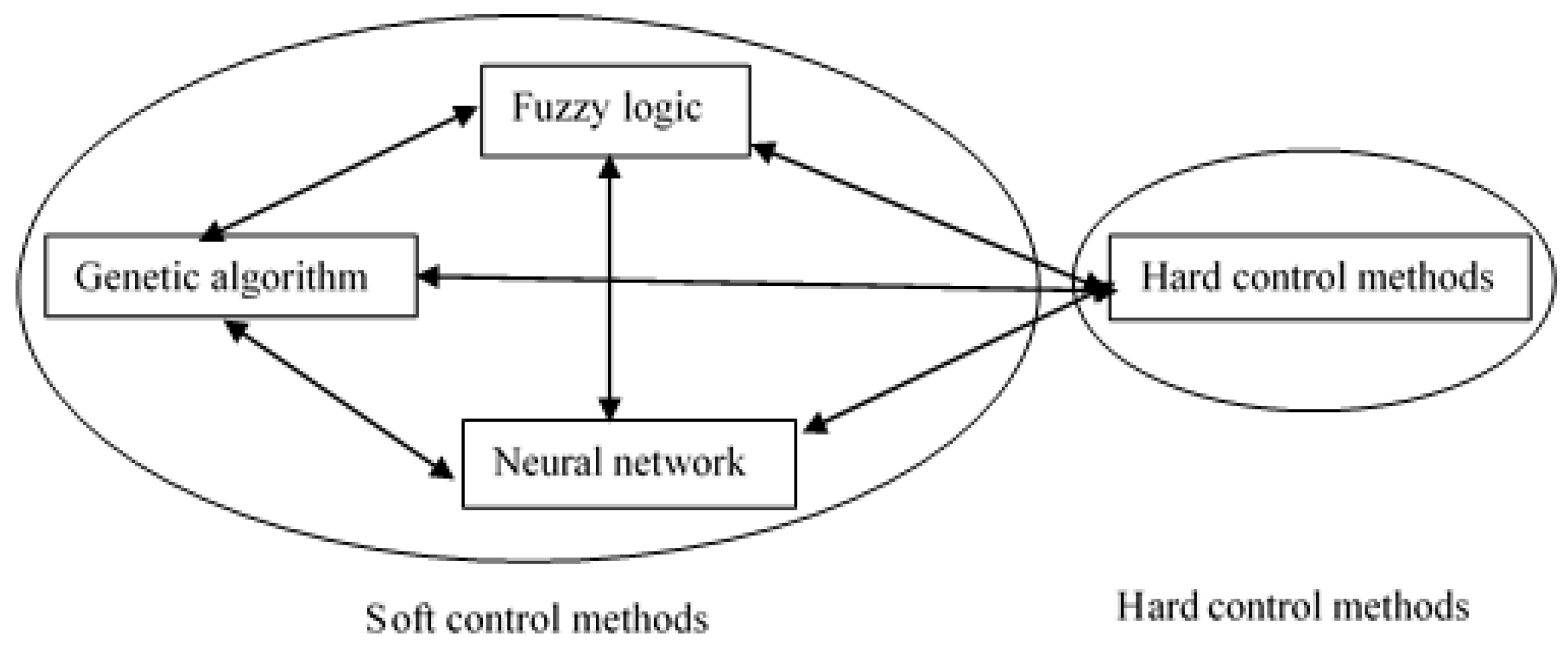
Figure 6.
The schematic diagram of typical HVAC system.
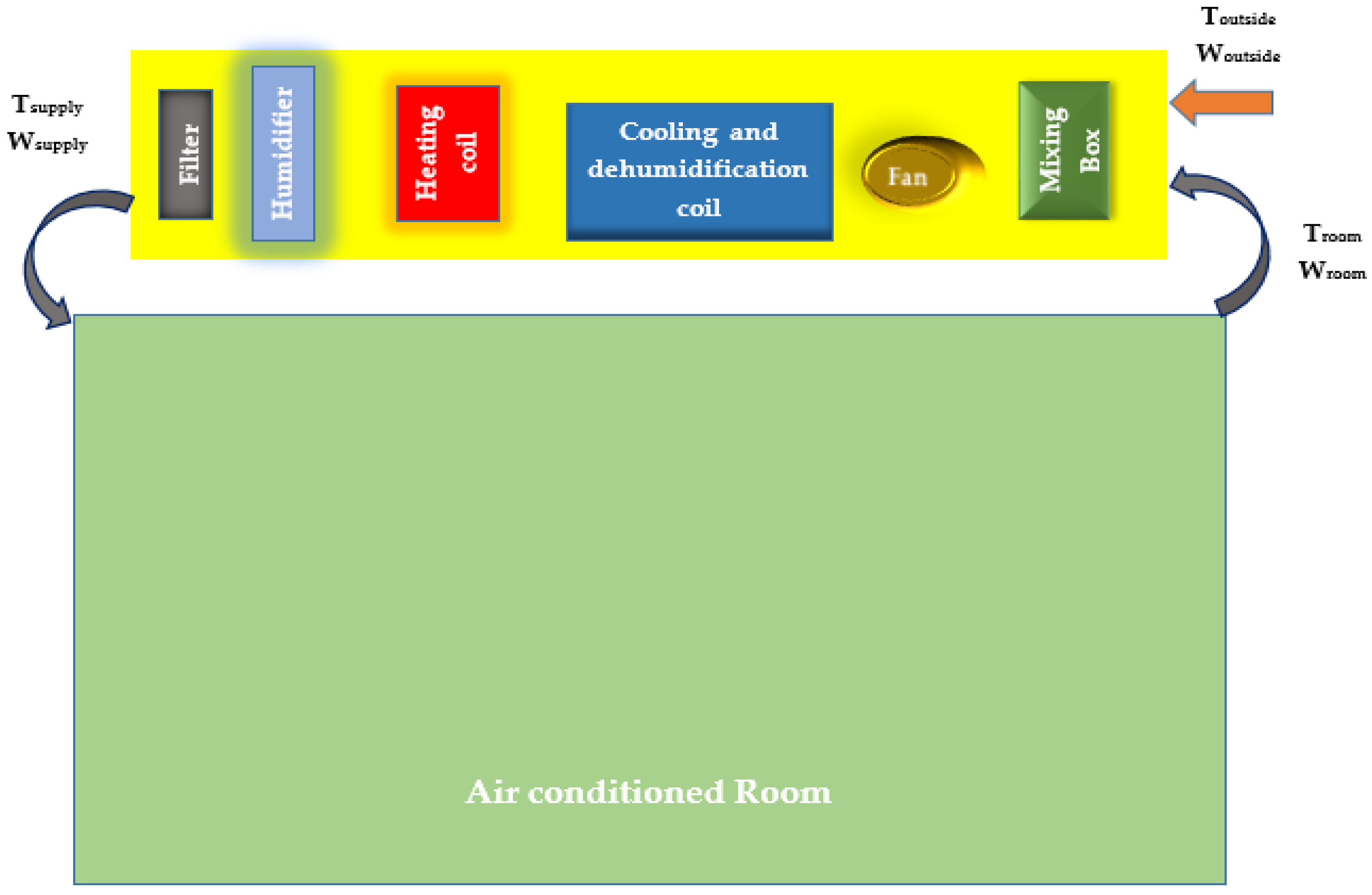
Figure 7.
The schematic diagram of the overall cooling system in summer operation season.

Figure 8.
The schematic diagram of the overall heating system in winter operation season.

Figure 9.
Temperature of the controlled zone in summer operation season by (a) FCM controller (b) PID controller.
Figure 9.
Temperature of the controlled zone in summer operation season by (a) FCM controller (b) PID controller.

Figure 10.
Humidity ratio of the controlled zone in summer operation season by (a) FCM controller (b) PID controller.
Figure 10.
Humidity ratio of the controlled zone in summer operation season by (a) FCM controller (b) PID controller.

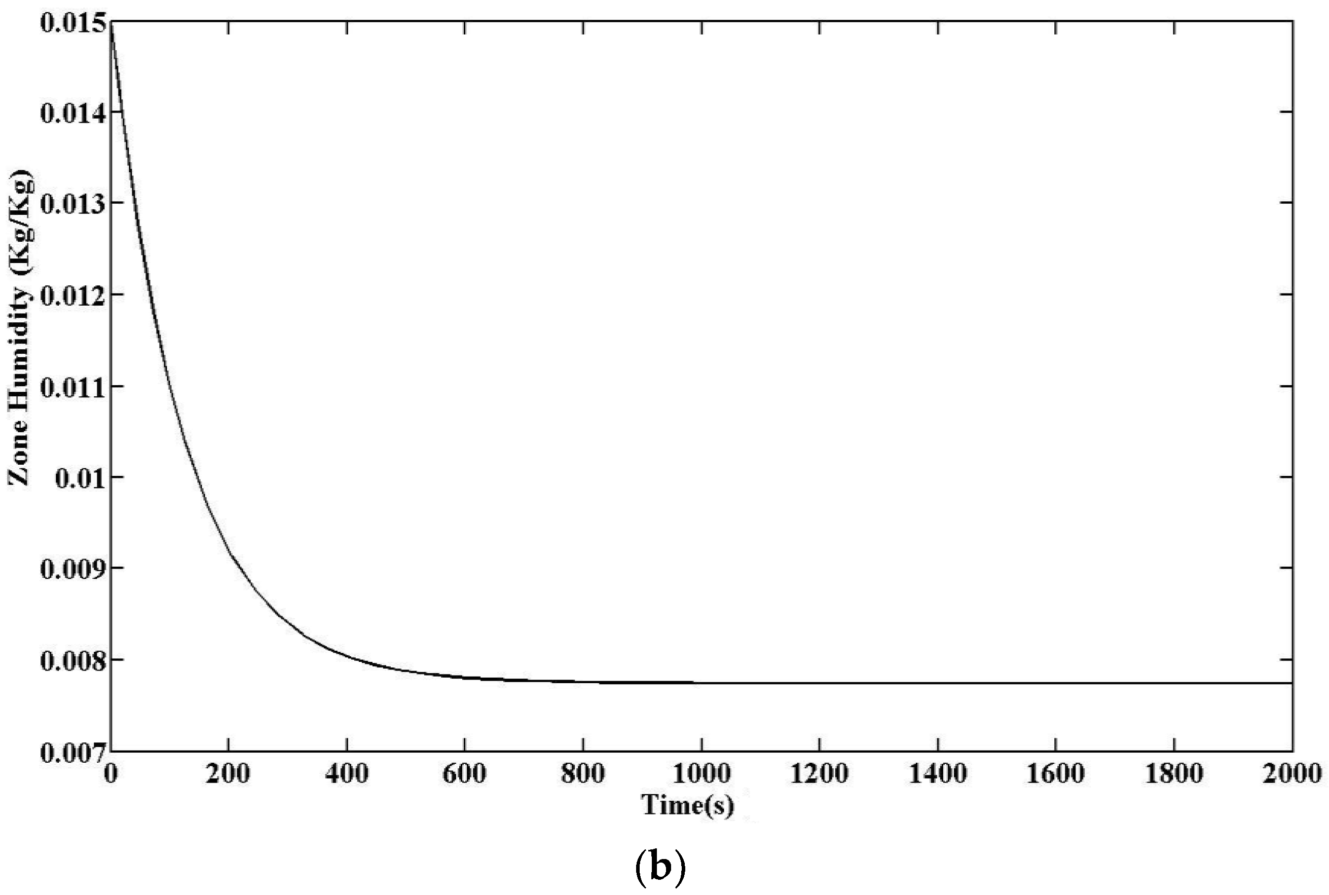
Figure 11.
Supply air temperature of the controlled zone in summer operation season by (a) FCM controller (b) PID controller.
Figure 11.
Supply air temperature of the controlled zone in summer operation season by (a) FCM controller (b) PID controller.
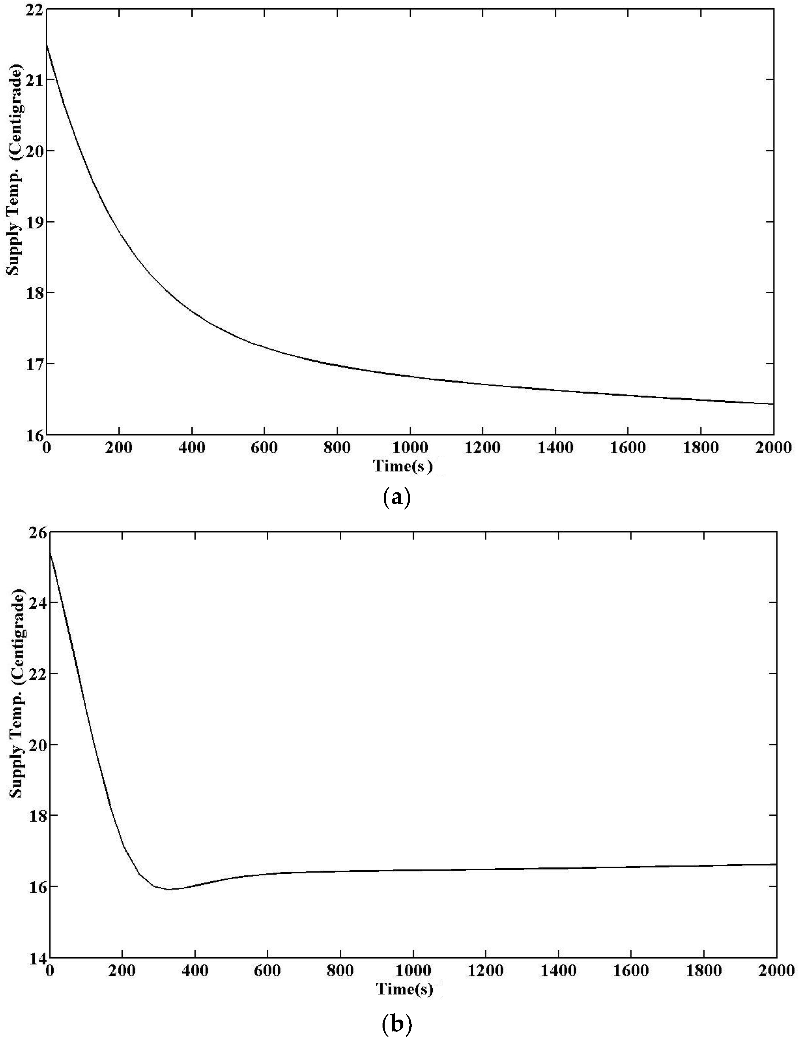
Figure 12.
Supply humidity ratio of the controlled zone in summer operation season by (a) FCM controller (b) PID controller.
Figure 12.
Supply humidity ratio of the controlled zone in summer operation season by (a) FCM controller (b) PID controller.
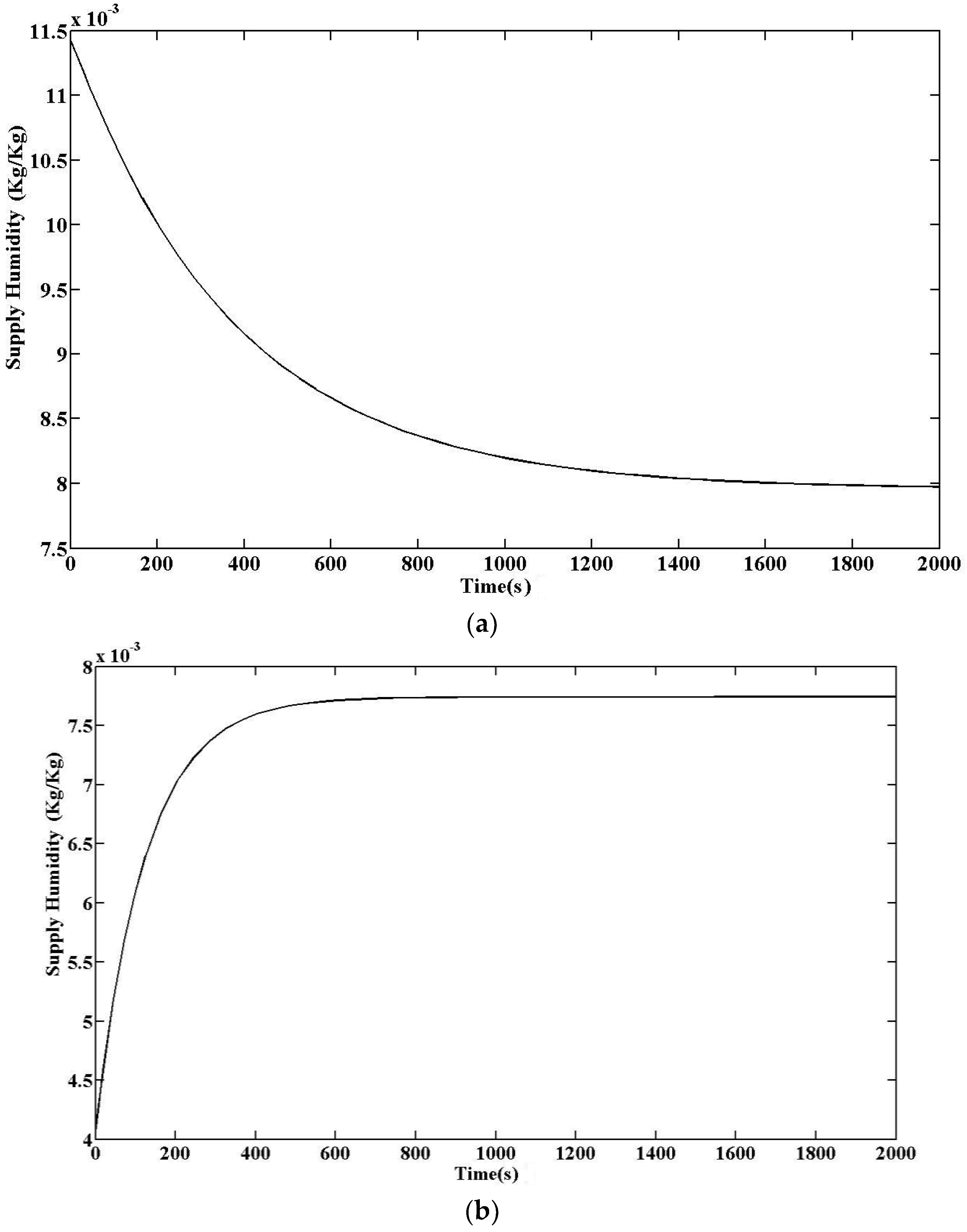
Figure 13.
Temperature of the controlled zone in winter operation season by (a) FCM controller (b) PID controller.
Figure 13.
Temperature of the controlled zone in winter operation season by (a) FCM controller (b) PID controller.


Figure 14.
Humidity ratio of the controlled zone in winter operation season by (a) FCM controller (b) PID controller.
Figure 14.
Humidity ratio of the controlled zone in winter operation season by (a) FCM controller (b) PID controller.

Figure 15.
Supply air temperature of the controlled zone in winter operation season by (a) FCM controller (b) PID controller.
Figure 15.
Supply air temperature of the controlled zone in winter operation season by (a) FCM controller (b) PID controller.
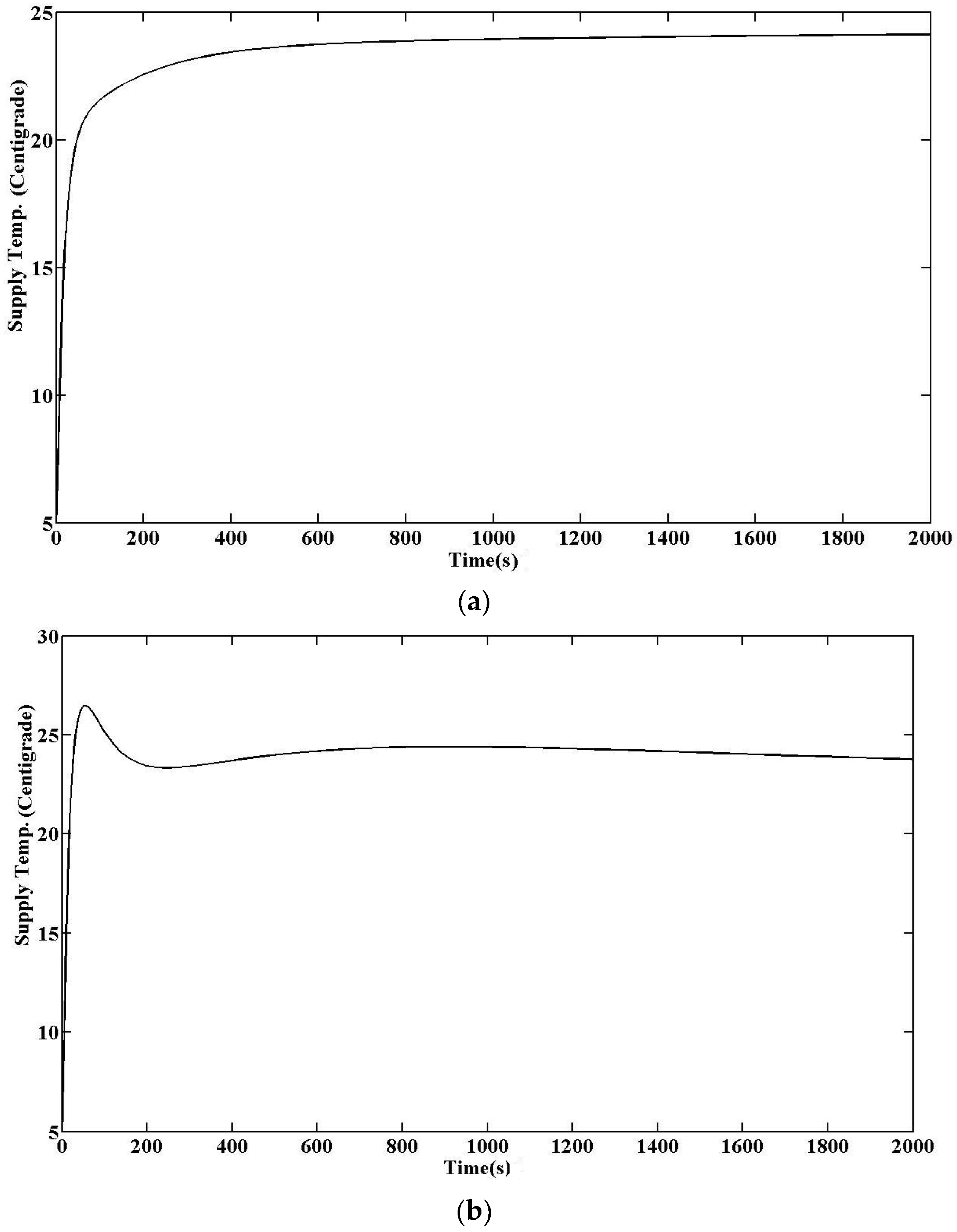
Figure 16.
Supply humidity ratio of the controlled zone in winter operation season by (a) FCM controller (b) PID controller.
Figure 16.
Supply humidity ratio of the controlled zone in winter operation season by (a) FCM controller (b) PID controller.


Figure 17.
The model of the DX A/C system.

Figure 18.
Air conditioned room temperature [91].
Figure 18.
Air conditioned room temperature [91].

Figure 19.
Air conditioned room humidity [91].
Figure 19.
Air conditioned room humidity [91].
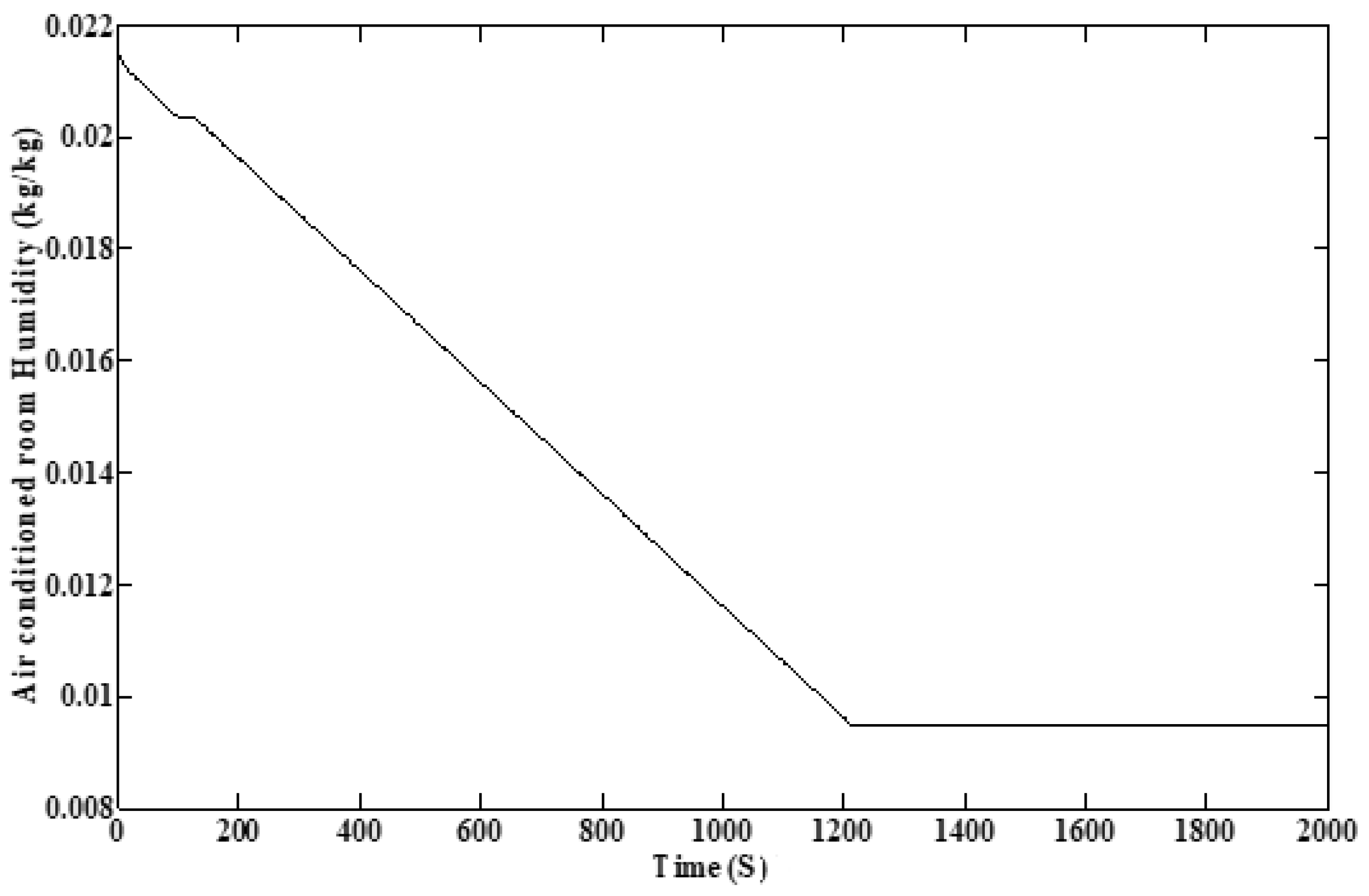
Figure 20.
Air conditioned room temperature in a set point tracking test with changes of set point to 23 °C [91].
Figure 20.
Air conditioned room temperature in a set point tracking test with changes of set point to 23 °C [91].

Figure 21.
Air conditioned room temperature in a disturbance rejection test [91].
Figure 21.
Air conditioned room temperature in a disturbance rejection test [91].
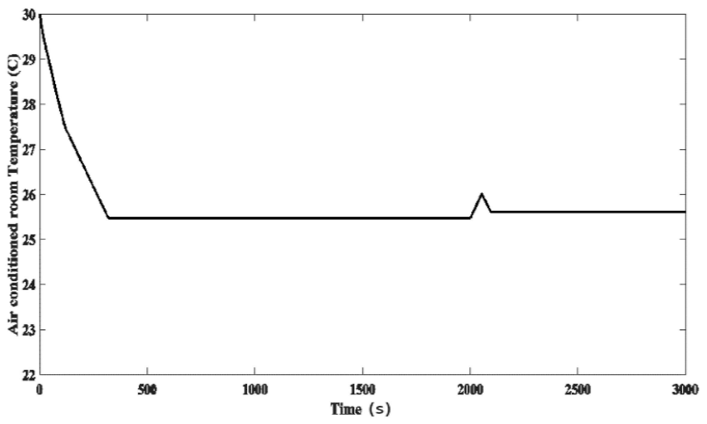
Figure 22.
Air conditioned room humidity in a disturbance rejection test [91].
Figure 22.
Air conditioned room humidity in a disturbance rejection test [91].
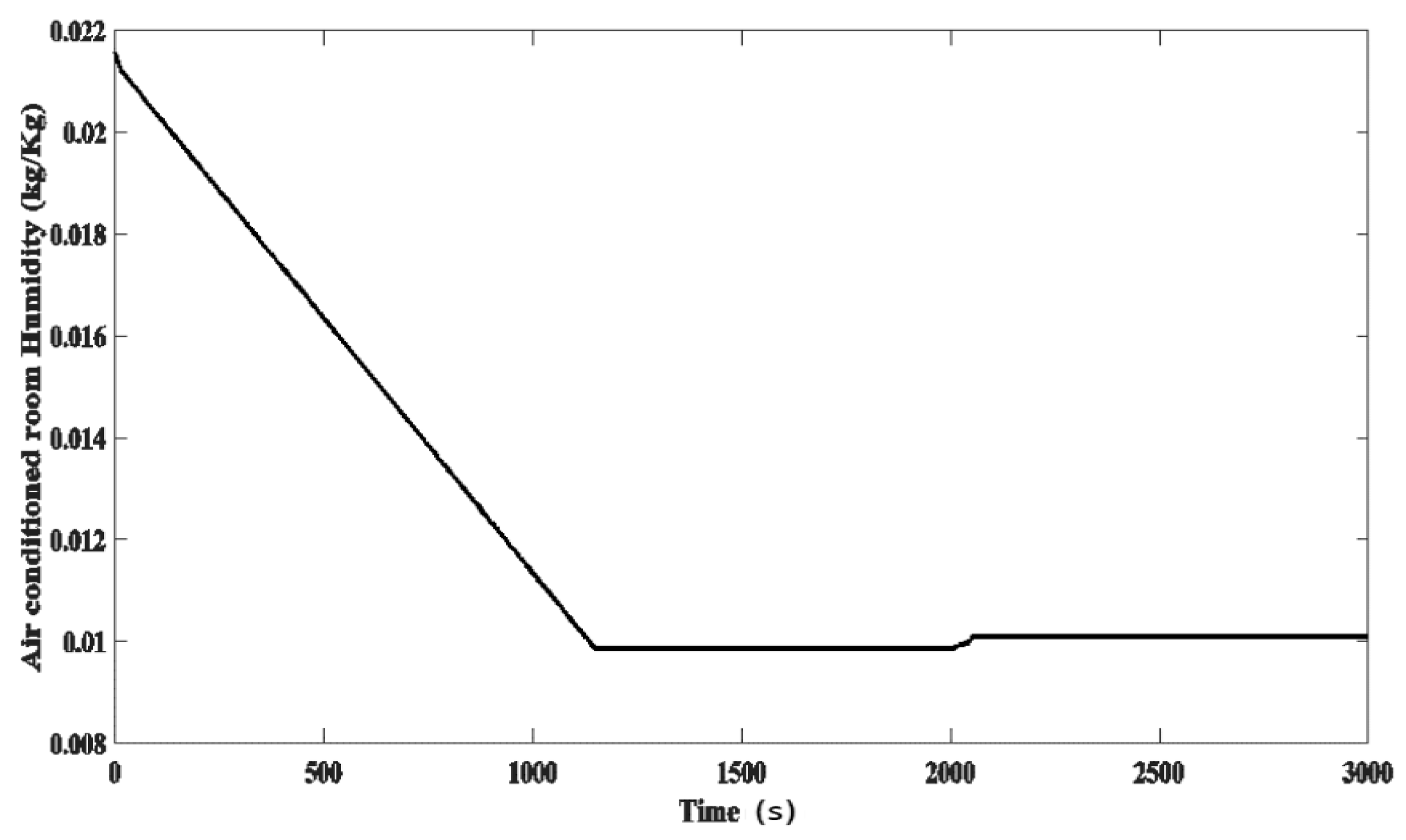

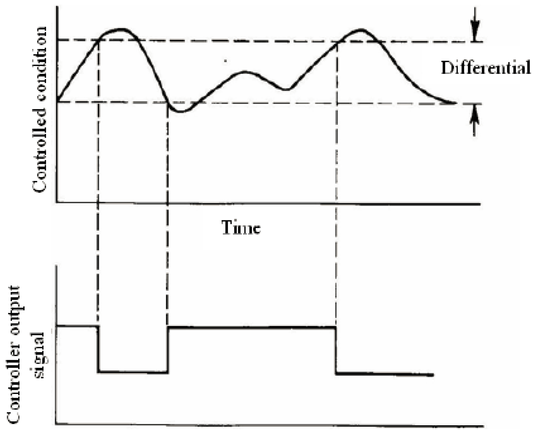
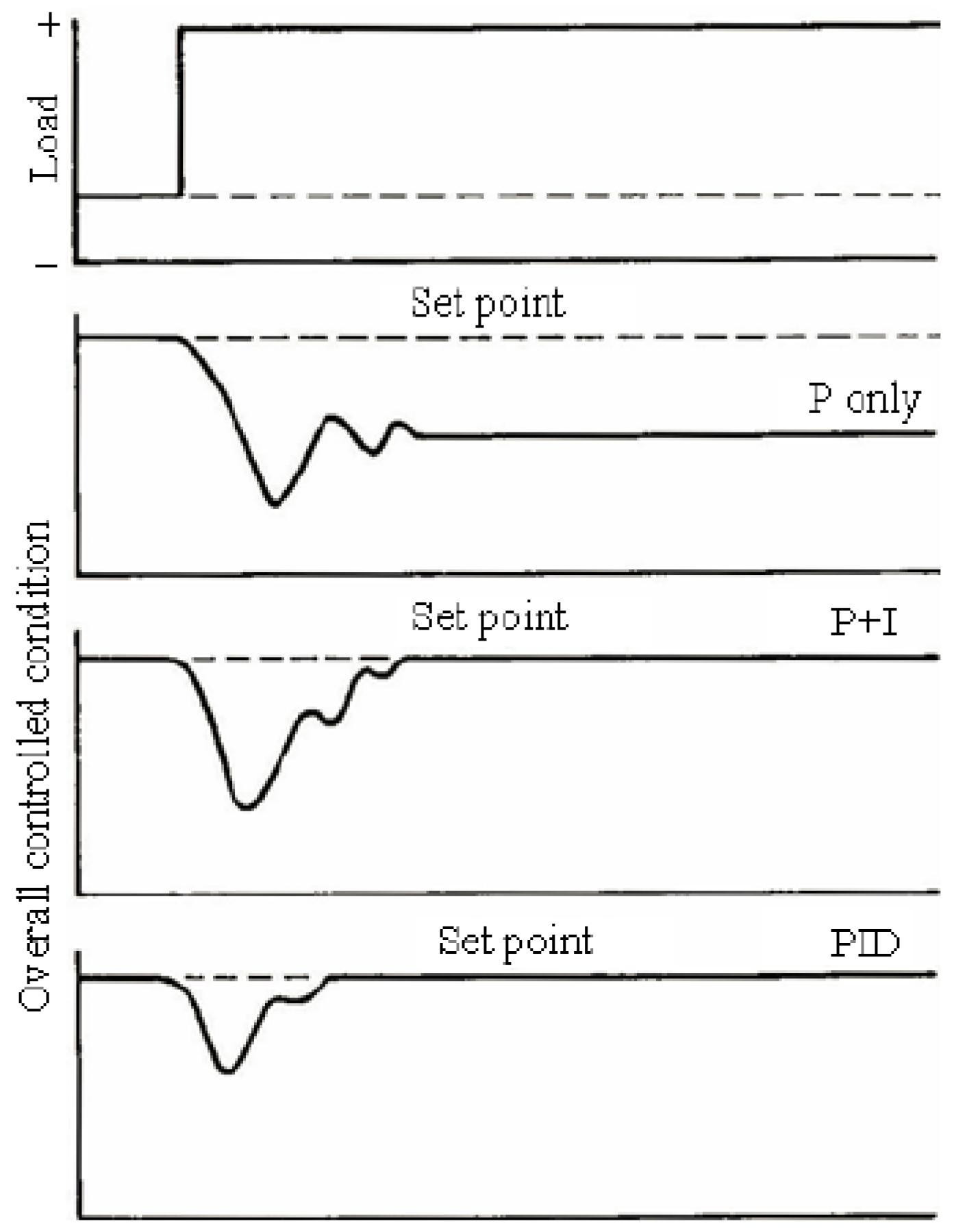
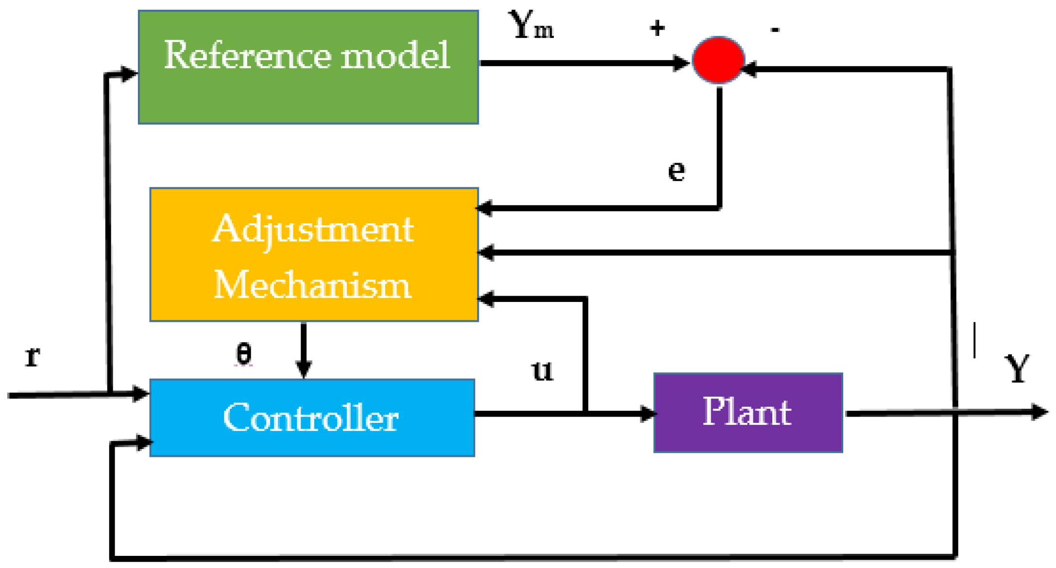
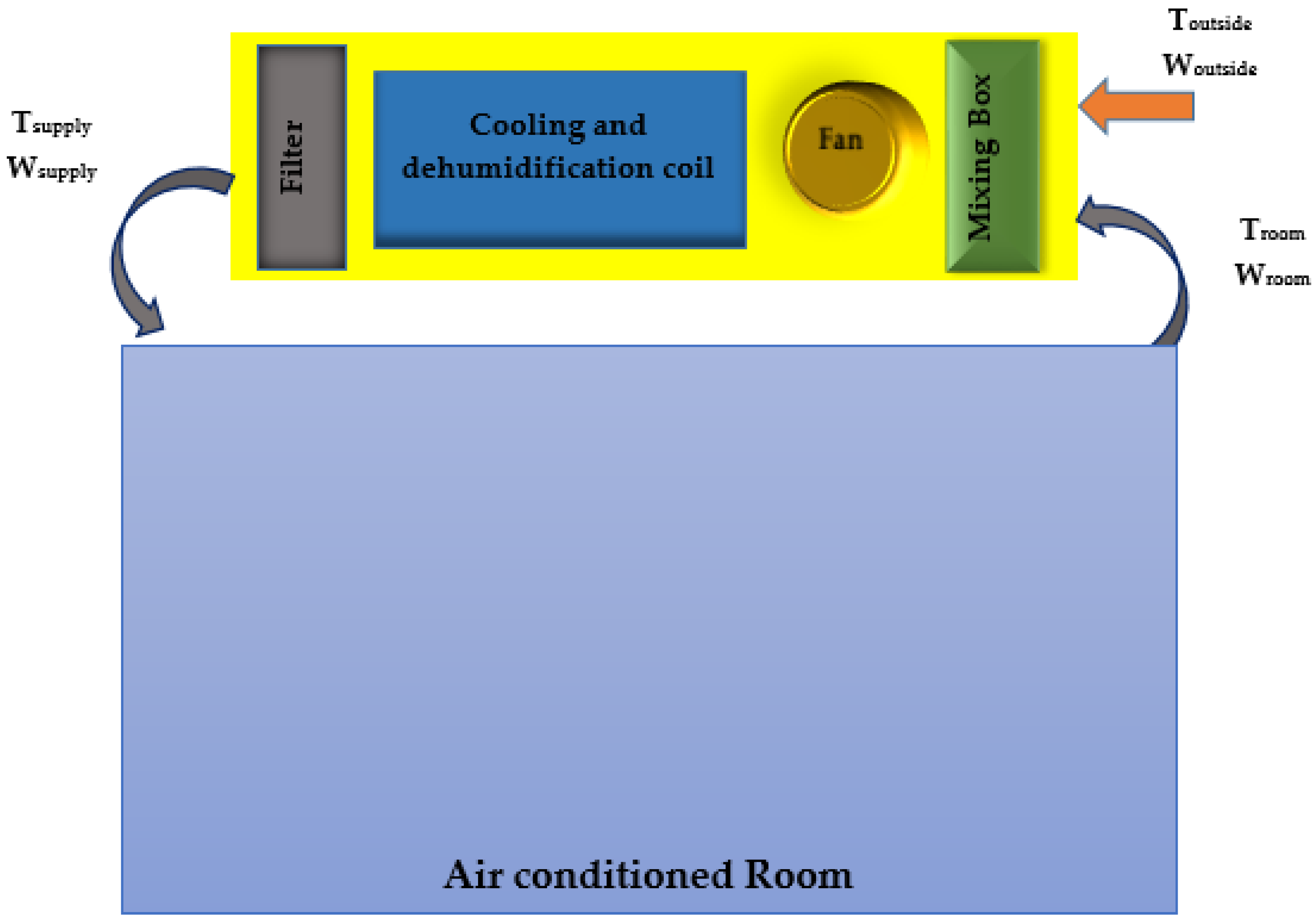
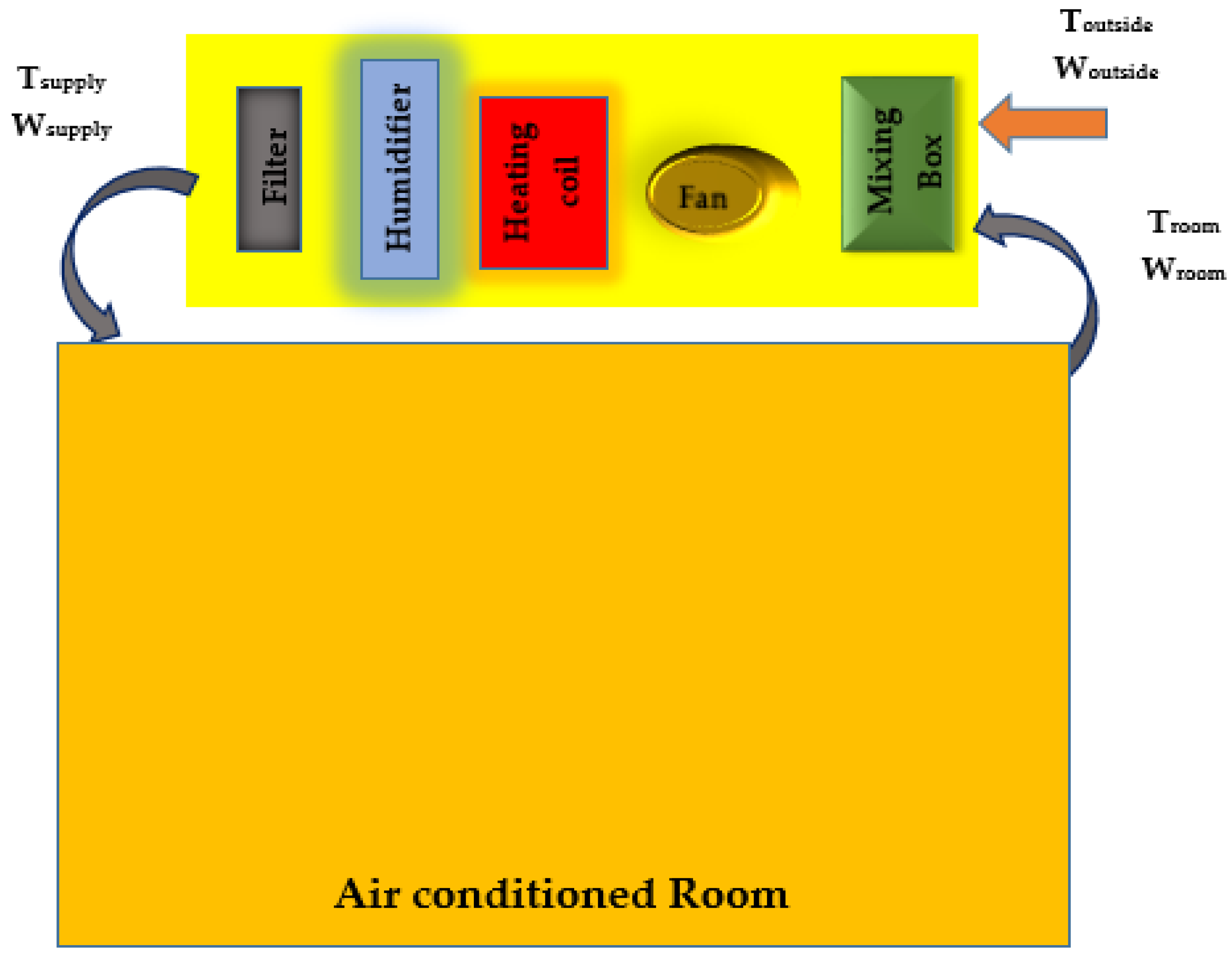
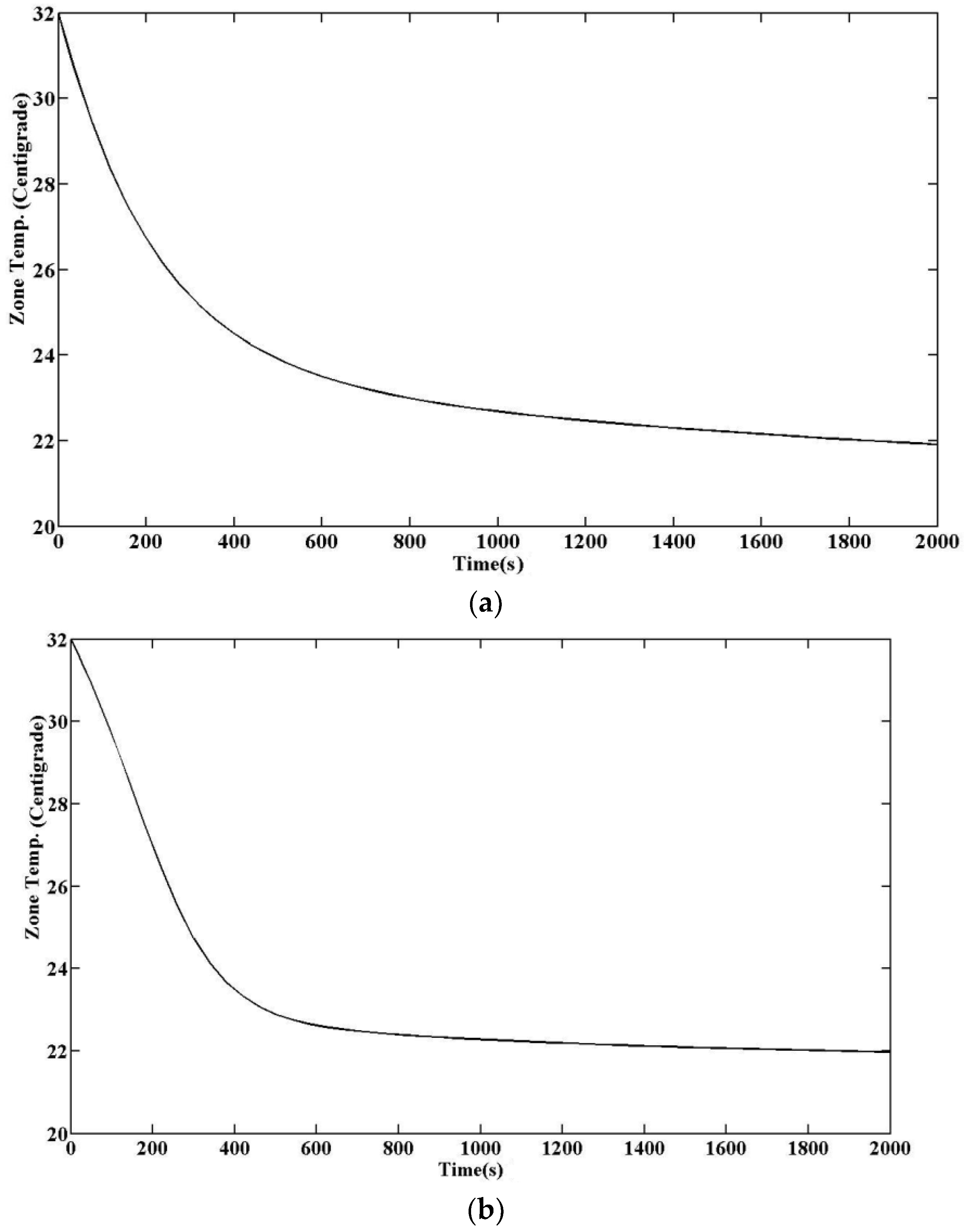
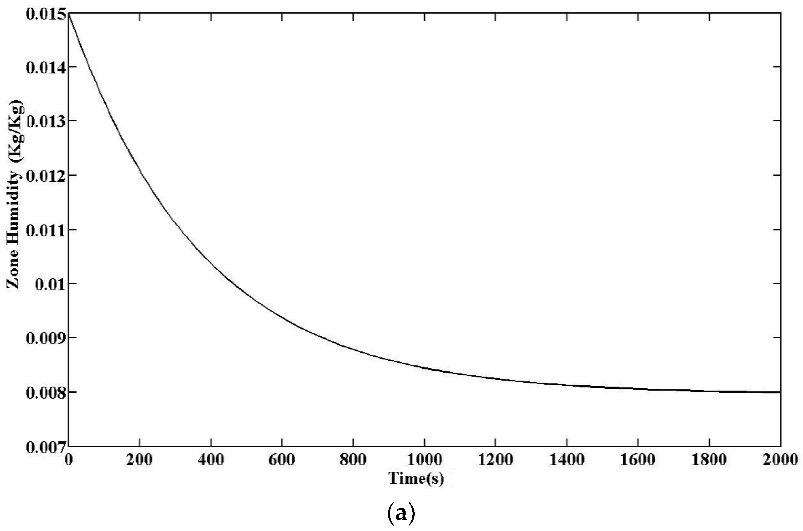
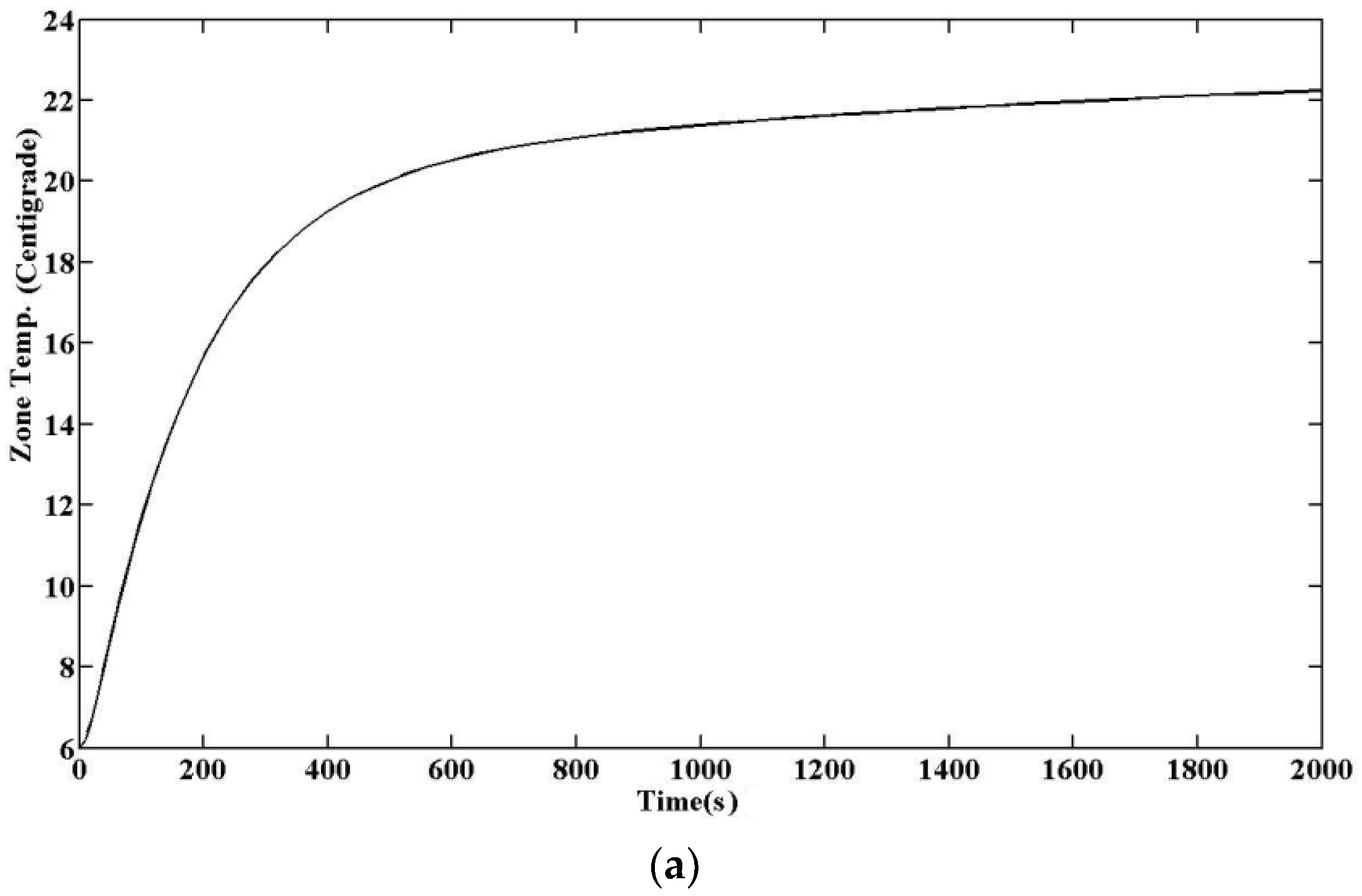
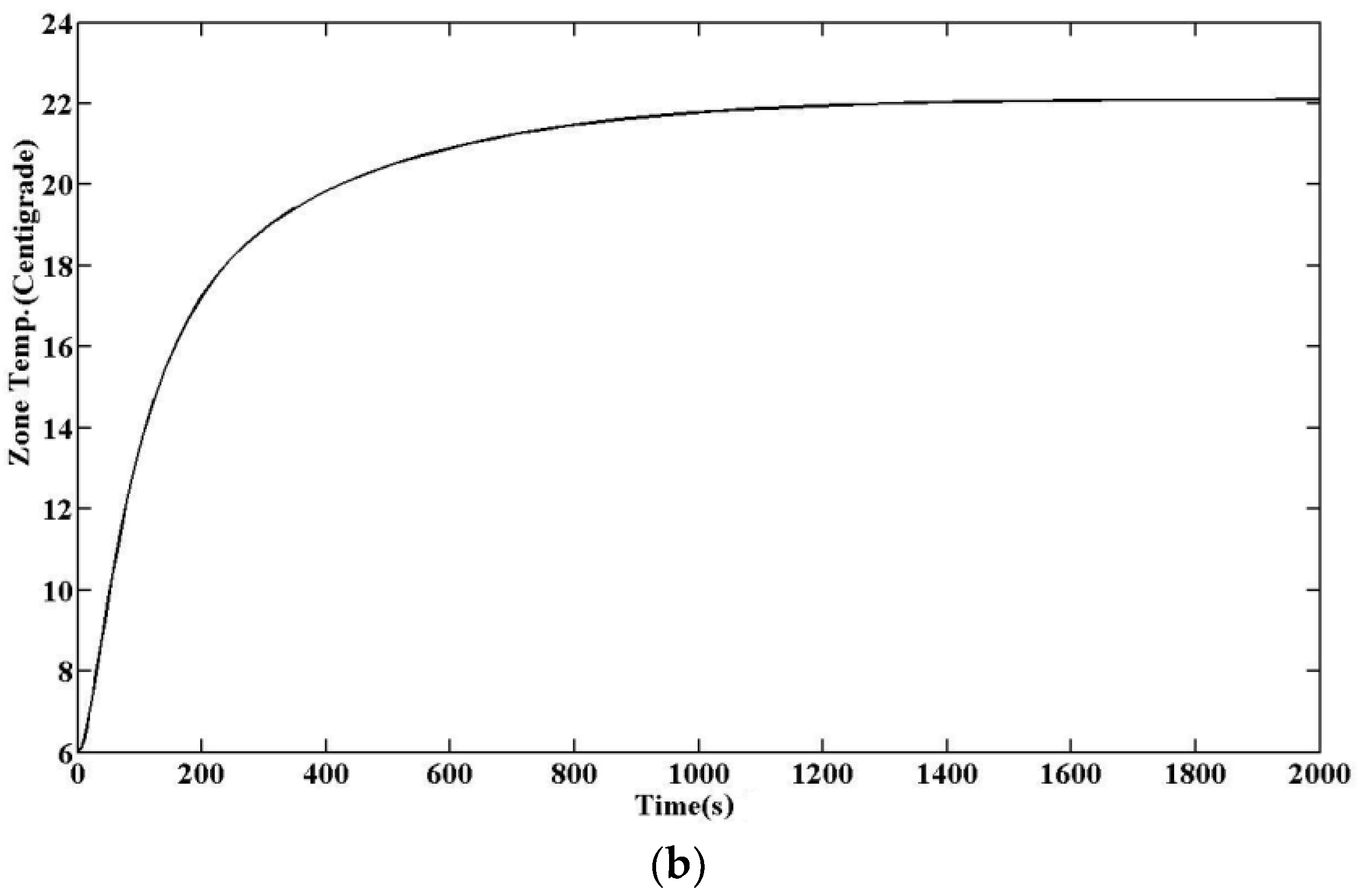
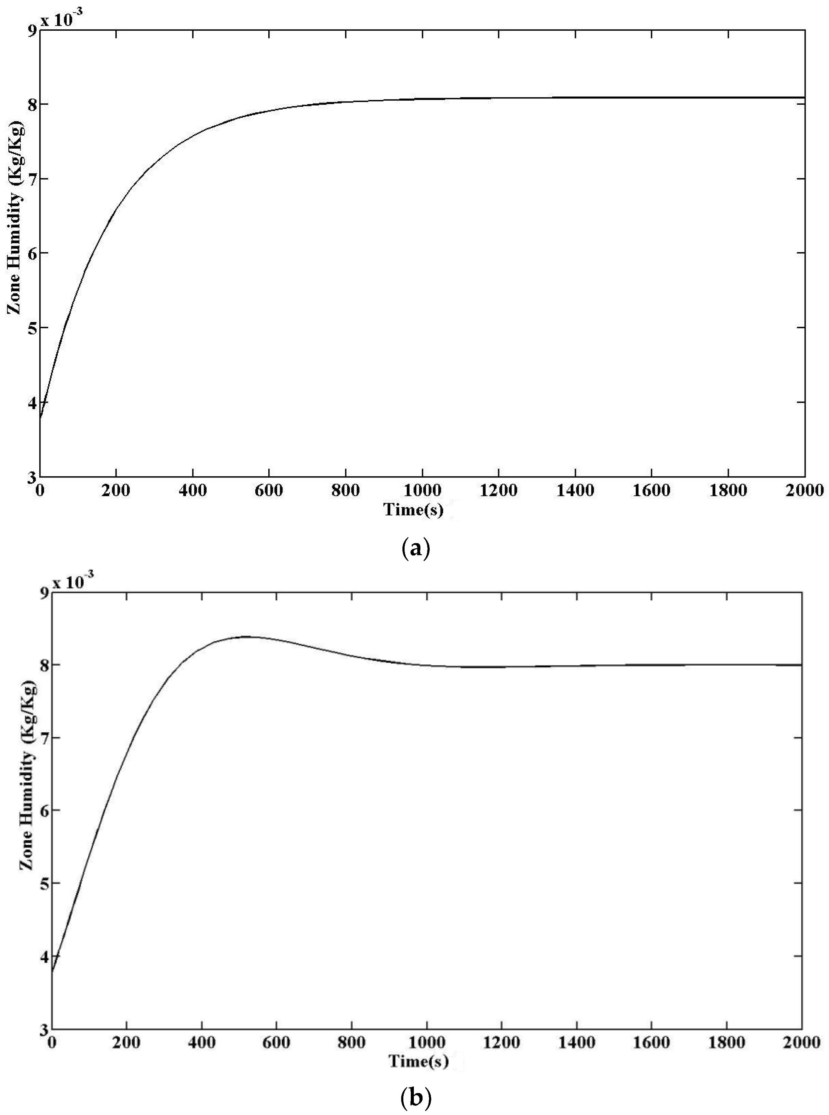
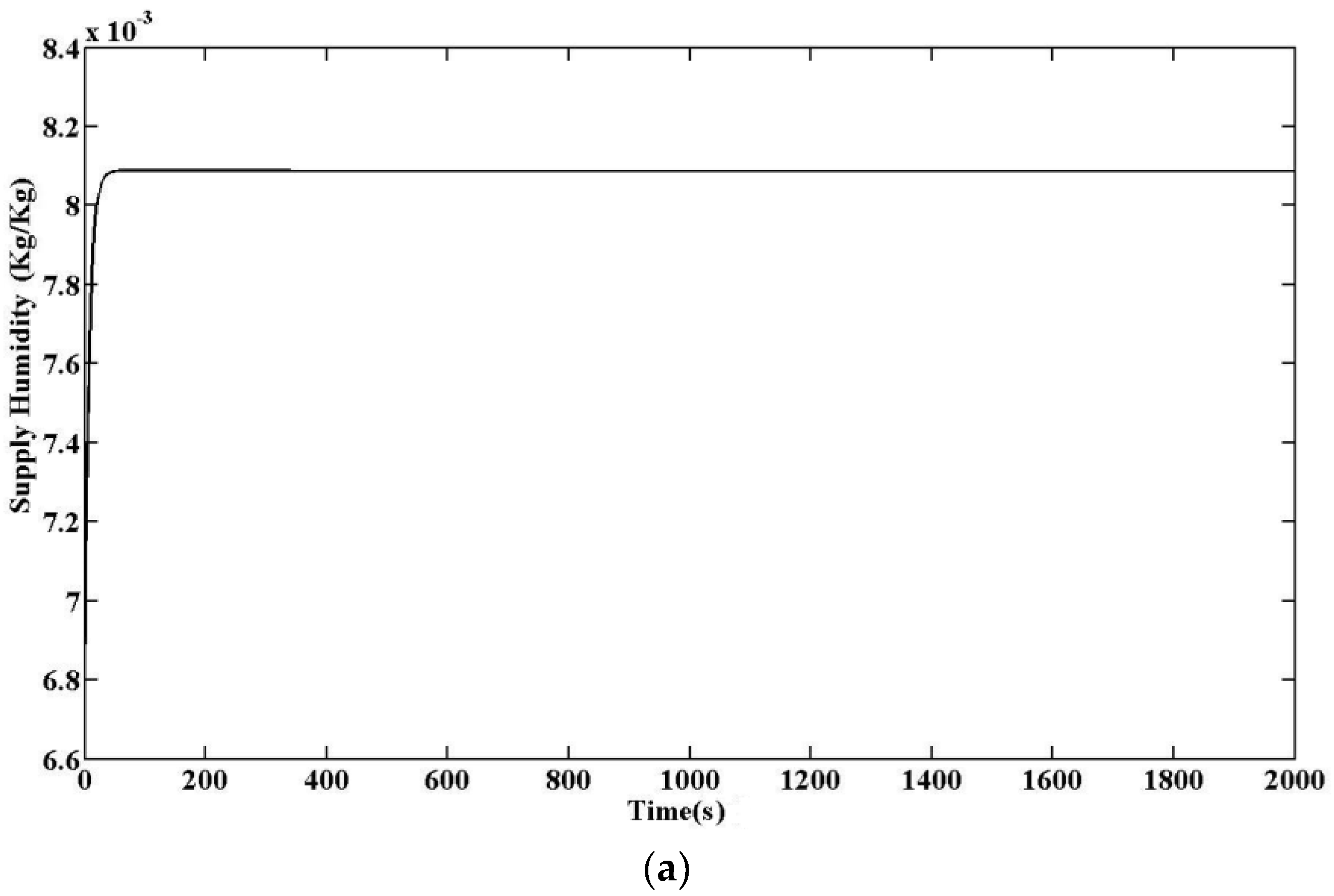
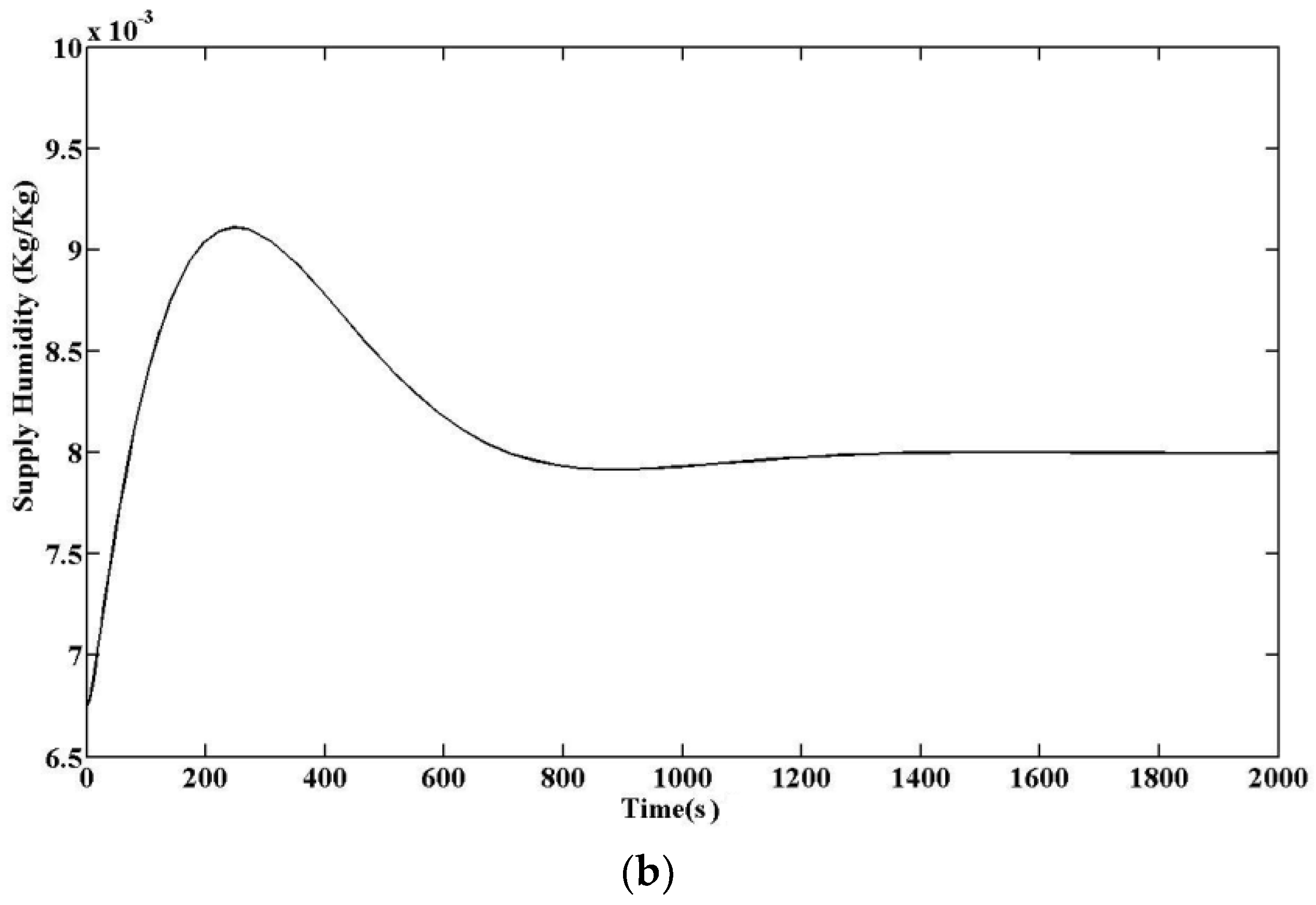
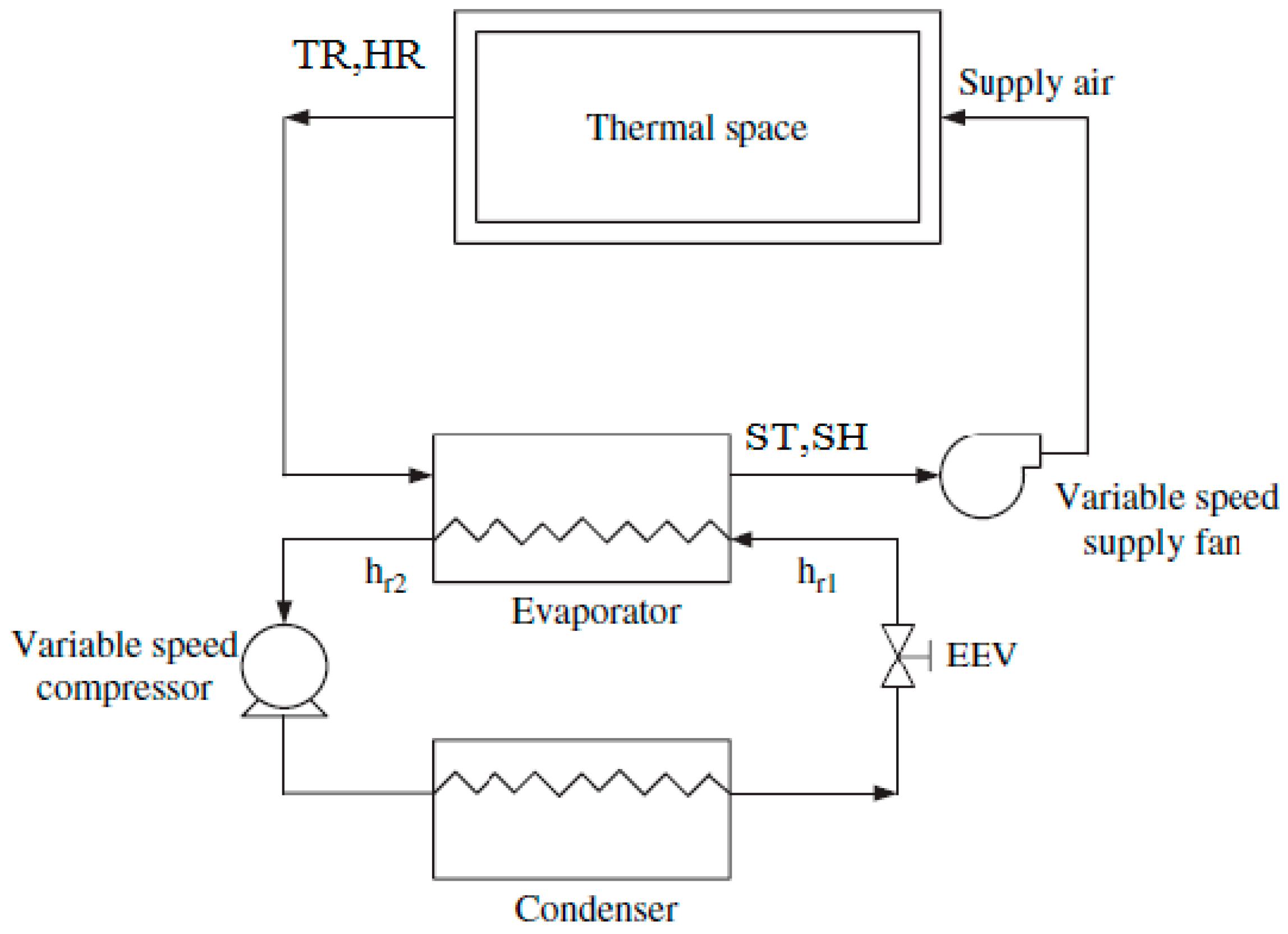
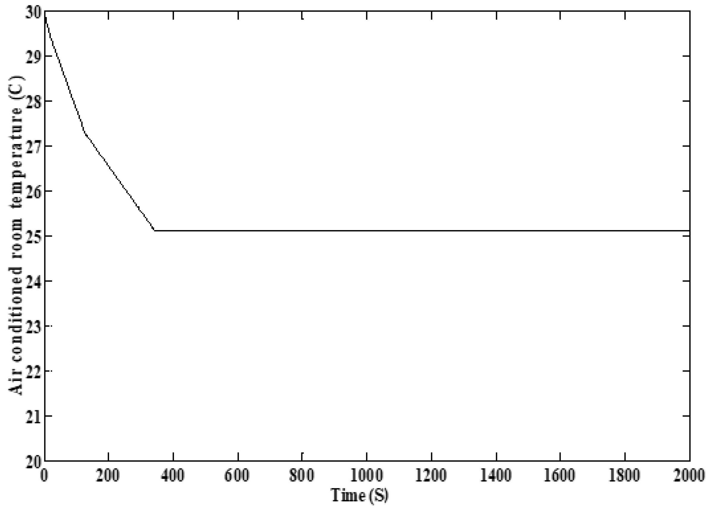
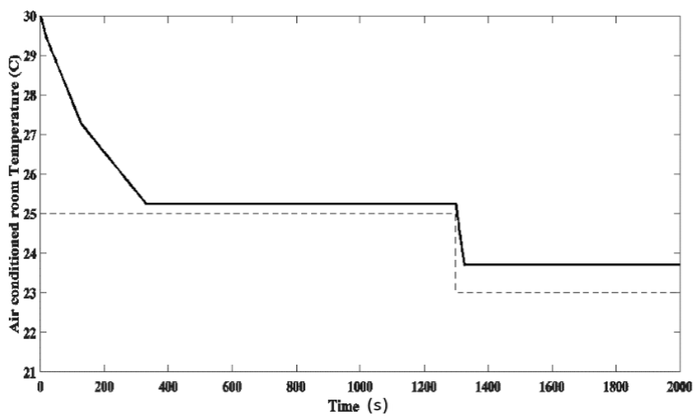
Table 1.
Advantages and disadvantages of classical control techniques.
| Control Method | Advantage | Disadvantage |
|---|---|---|
| On/Off control | ||
| PID control |
|
Table 2.
Advantages and disadvantages of optimal control techniques.
| Control Method | Advantage | Disadvantage |
|---|---|---|
| Optimal controls |
|
Table 3.
Advantages and disadvantages of robust control techniques.
| Control Method | Advantage | Disadvantage |
|---|---|---|
| Robust control |
|
Table 4.
Advantages and disadvantages of adaptive control techniques.
| Control Method | Advantage | Disadvantage |
|---|---|---|
| Adaptive control |
|
Table 5.
Advantages and disadvantages of nonlinear control technique.
| Control Method | Advantage | Disadvantage |
|---|---|---|
| Nonlinear control |
|
|
Table 6.
Different methods for non-linear control systems.
| Methods | Advantageous | Disadvantageous |
|---|---|---|
| state-feedback controller(Linearization around an operating point) |
|
|
| Compensation of static nonlinearities |
|
|
| Linearization by local feedback |
|
|
| Input-to-state linearization |
|
|
| Input-to-output linearization |
|
|
| Lyapunov redesign |
|
|
| Backstepping |
|
|
| Sliding-mode control |
|
|
| Relay control |
|
|
| Gain scheduling (open-loop adaptive scheme) |
|
|
| Adaptive Control (closed-loop adaptive scheme) |
|
|
| Neural network control |
|
|
| Fuzzy control |
|
|
Table 7.
Advantages and disadvantages of model predictive control techniques.
| Control Method | Advantage | Disadvantage |
|---|---|---|
| MPC method |
|
Table 8.
Advantages and disadvantages of artificial neural network control techniques.
| Control Method | Advantage | Disadvantage |
|---|---|---|
| ANN method |
|
|
Table 9.
Advantages and disadvantages of fuzzy logic control techniques.
| Control Method | Advantage | Disadvantage |
|---|---|---|
| FL method |
|
|
Table 10.
Merits and demerits of genetic algorithm control techniques.
| Control Method | Advantage | Disadvantage |
|---|---|---|
| GA method |
|
|
© 2018 by the authors. Licensee MDPI, Basel, Switzerland. This article is an open access article distributed under the terms and conditions of the Creative Commons Attribution (CC BY) license (http://creativecommons.org/licenses/by/4.0/).
Share and Cite
MDPI and ACS Style
Behrooz, F.; Mariun, N.; Marhaban, M.H.; Mohd Radzi, M.A.; Ramli, A.R. Review of Control Techniques for HVAC Systems—Nonlinearity Approaches Based on Fuzzy Cognitive Maps. Energies 2018, 11, 495. https://doi.org/10.3390/en11030495
AMA Style
Behrooz F, Mariun N, Marhaban MH, Mohd Radzi MA, Ramli AR. Review of Control Techniques for HVAC Systems—Nonlinearity Approaches Based on Fuzzy Cognitive Maps. Energies. 2018; 11(3):495. https://doi.org/10.3390/en11030495
Chicago/Turabian StyleBehrooz, Farinaz, Norman Mariun, Mohammad Hamiruce Marhaban, Mohd Amran Mohd Radzi, and Abdul Rahman Ramli. 2018. "Review of Control Techniques for HVAC Systems—Nonlinearity Approaches Based on Fuzzy Cognitive Maps" Energies 11, no. 3: 495. https://doi.org/10.3390/en11030495
Note that from the first issue of 2016, this journal uses article numbers instead of page numbers. See further details here.