Height Adjustment of Vehicles Based on a Static Equilibrium Position State Observation Algorithm †

1
Automotive Research Institute, School of Mechanical Engineering, Institute of Technology (BIT), 5 South Zhongguancun Street, Haidian District, Beijing 100081, China
2
National Engineering Laboratory for Electric Vehicles and Collaborative Innovation Center of Electric Vehicles in Beijing, Beijing Institute of Technology (BIT), 5 South Zhongguancun Street, Haidian District, Beijing 100081, China
*
Author to whom correspondence should be addressed.
†
This paper is an extended version of our paper published in Gao Z.P.; Nan J.R.; Xv X.L.; Wang J. Research on vehicle height adjustment control algorithm of air suspension based on UKF state observation algorithm. International Symposium on Electric Vehicles, Stockholm, Sweden, 26–29 July 2017.
Energies 2018, 11(2), 455; https://doi.org/10.3390/en11020455
Submission received: 20 January 2018
/
Revised: 8 February 2018
/
Accepted: 9 February 2018
/
Published: 21 February 2018
(This article belongs to the Special Issue The International Symposium on Electric Vehicles (ISEV2017))
Abstract
:In this paper, a static state observer algorithm based on the static equilibrium position is proposed, which can realize accurate control of electric vehicle height adjustment with existing road excitation. The existence of road excitation can lead to deflection variation of the electronically controlled air suspension (ECAS). The use of only dynamic deflection as the reference for the electric vehicle height adjustment will produce great errors. Therefore, this paper provides an observation algorithm, which can realize the accurate control of vehicle height. Firstly, the static equilibrium position equation of suspension is derived according to the theory of hydrodynamics and characteristics of pneumatic chamber. Secondly, a vehicle dynamics model with seven degrees of freedom (7-DOF) is established and the kinetic equations are discretized. Then, the unscented Kalman filter (UKF) algorithm is used to obtain the static equilibrium position of vehicle. According to the vehicle static equilibrium position obtained by UKF, the height of the vehicle is adjusted by using a fuzzy controller. The simulation and experimental results show that this proposed algorithm can realize the control of vehicle height with an accuracy of over 96%, which ensures the excellent driving performance of vehicles under different road conditions.
1. Introduction
The electric vehicle semi-active suspension system has attracted more and more attention [1,2,3,4] because it can effectively improve the ride comfort, handling stability and trafficability to ensure the comfort of passengers, the integrity of goods and the safety of driving [5,6,7]. The electronically controlled air suspension (ECAS) belongs to the semi-active suspension class. It has been widely used in commercial vehicles [8], railway vehicles [9], passenger vehicles [10] and agricultural machines [11,12] because of its advantages of adjustable stiffness and height. In the past few years, the research on air suspension systems has mainly focused on three aspects: air suspension analysis modeling [13,14,15,16,17], electronic control system [18,19,20,21,22] and vehicle height control algorithms [23,24,25,26,27,28,29,30].
In the 1980s, European countries and the U.S. designed electronic control units on the basis of the traditional passive air suspension so that the ECAS concept was formed. With the development of electronic control technology, more and more attention has been paid to the improvement of vehicle driving performance. New progress has been made in the study of vehicle height and vehicle performance and many scholars have concentrated on the study of vehicle height control algorithms. The fault tolerant control algorithm was applied to the height adjustment of air suspension by Kim and Lee et al. and effective control effect was achieved [28,29]. Subsequently, they designed a vehicle sliding mode controller based on feedback linearization and established four state observers for internal pressure of the air suspension in order to improve the accuracy of vehicle height adjustment [30]. Chen et al. established a kinetic model of 1/4 air suspension for agricultural vehicles. The single neuron adaptive PID (SNA-PID) controller was used to adjust the height of vehicles with the existence of road excitation by using height sensors. Compared with the traditional fuzzy-PID controller, the accuracy and the efficiency of this control algorithm was effectively improved [11]. Xu et al. established a mathematical model of a vehicle height adjustment system with random disturbance which was regarded as a nonlinear system. This system was decoupled by using the theory of differential geometry and the variable structure control (VSC) method was used to stabilize the system [22]. Then, Xu et al. used three height sensors to establish a three points measuring system so as to establish a mathematical model of vehicle height adjustment. On this basis, the hierarchical control method was proposed by using the VSC technique and fuzzy control theory. The application of this method ensured the stabilization of the system and met the height requirements [23]. Sun et al. established a nonlinear model of vehicle height adjustment with a variable mass inflation/deflation system based on the theory of vehicle system dynamics and thermodynamics. Then, the framework of mixed logical dynamics (MLD) was used to solve the continuous/discrete dynamics problems by controlling the switching state of the solenoid valve in the process of vehicle height adjustment [24]. On the basis of the previous results, they proposed a correction algorithm based on pulse width modulation (PWM) technology, which was used to control the duration of the solenoid valve switch state, so that the control accuracy of height, roll angle and pitch angle could be better realized in the process of height adjustment. The experimental results proved that the control algorithm could control the vehicle attitude [25,27].
However, little attention has been paid to the relationship between the vehicle height and the mass flow rate in the process of pneumatic spring inflating/deflating. The suspension static equilibrium position refers to the ratio of suspension load to suspension stiffness when the vehicle is stationary. The static equilibrium position is constant as long as the sprung mass and suspension stiffness remain constant. If there is no gas exchange and the mass flow in the pipeline is zero, the stiffness of the pneumatic spring is constant after the gas reaches its steady state through a self-balancing process. Therefore, the static equilibrium position is related to the inflating/deflating process. When a vehicle is running on a different road, the target height is different [24]. It’s necessary to adjust the vehicle height according to road conditions in real time, so as to ensure the good handling stability and trafficability of vehicles. If the reference variables selected are inaccurate or even lacking an effective reference to judge whether the vehicle height has reached its target value, it’s difficult to reasonably control the vehicle body attitude in the process of movement and ensure normal driving. In this case, the vehicle height sensors can only detect the changes of suspension dynamic deflections which is related to the road excitation, but it’s difficult to obtain the actual air suspension height changes caused by inflating/deflating. The static equilibrium position can be used to adjust the vehicle height because it doesn’t change without inflating/deflating. The main feature of this paper is the use of the static equilibrium position to realize precise adjustment of vehicle height under different road conditions.
The remainder of this paper is structured as follows: in Section 2, the principle of the ECAS system is introduced. A seven degrees of freedom (7-DOF) dynamic model of a vehicle is established. Then, a simulation model of ECAS is established. According to hydrodynamics theory and the pneumatic chamber characteristics, a mathematical model of the air suspension is established and the expression of suspension static equilibrium position is derived. The control strategy used in this paper is put forward in Section 3. Based on the discretization of dynamic equations and unscented transformation of state variables, the static equilibrium position of the suspension is obtained using the unscented Kalman filter (UKF) state observer. Then, the designed fuzzy controller is used to adjust the vehicle height. In Section 4, the dynamic model is verified by simulation. This model is simulated on the CarSim-AMESim-Simulink joint simulation platform using parameters obtained from CarSim and AMESim. Different excitation conditions in the simulation are set as follows: the vehicle height lifts/lowers 0.03 m without road excitation, the height rises 0.03 m when the vehicle is passing over a speed bump, the height falls 0.03 m when vehicle is running at 90 km/h speed on a B level typical road. In Section 5, vehicle experiments are carried out. The models and algorithm used for simulation are verified by real vehicle experiments. Then, the conclusions of the experiments and simulations are discussed and summarized in Section 6.
2. System Modeling
2.1. ECAS System
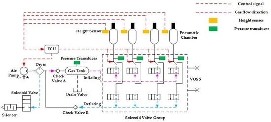
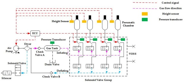
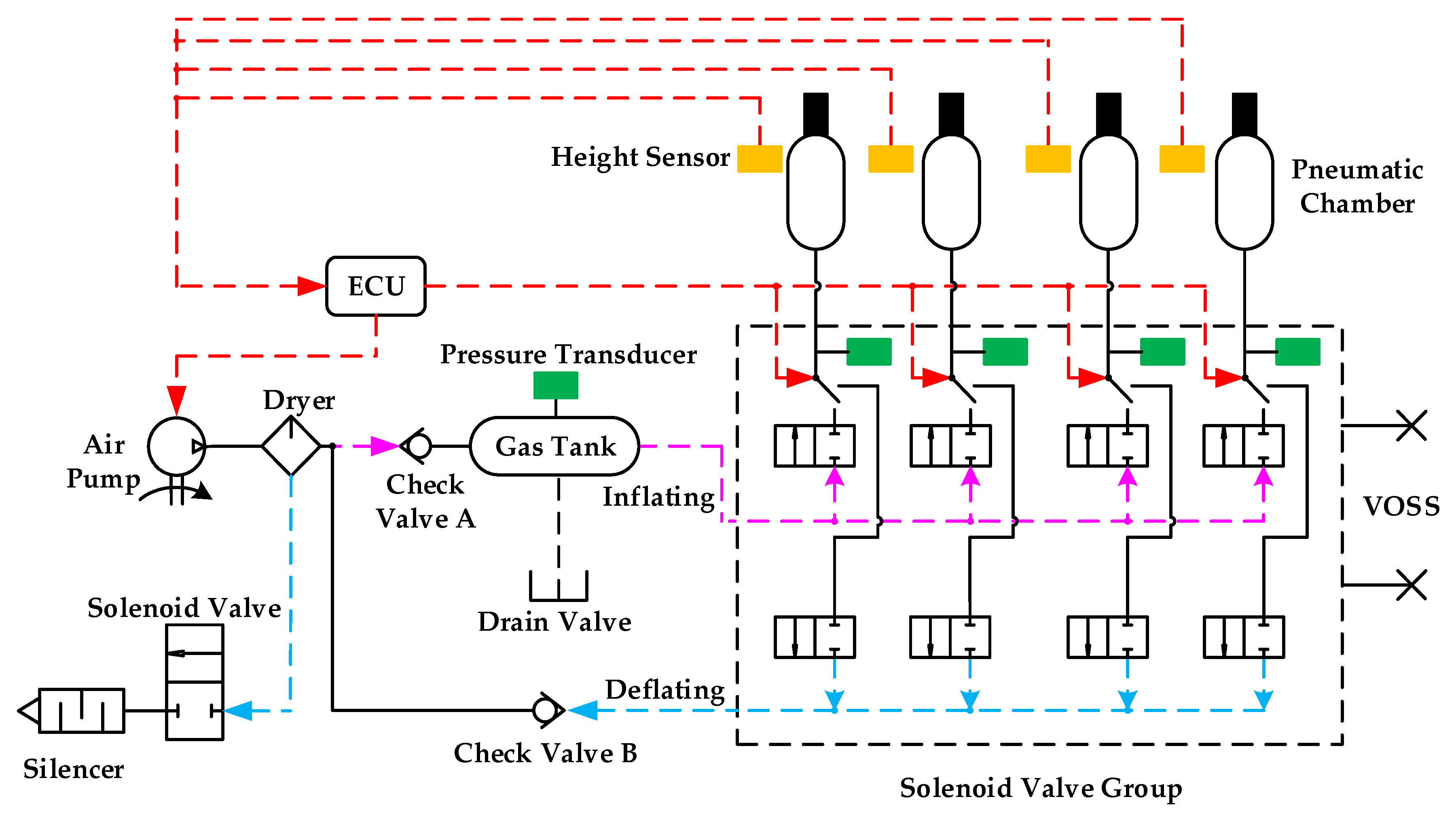
The main components of an ECAS system include the air suspension, ECU, gas tank, valves (including solenoid valve group and check valves), sensors (including height sensors and pressure sensors), air pump, dryer and silencer, etc. The schematic diagram of an ECAS system is shown in Figure 1.
The working principle of the ECAS system is described as follows: after receiving the height and pressure signals, the ECU determines the current state of the vehicle through signals such as speed and pedal signals, etc. The vehicle height can be adjusted by the switching operation of the solenoid valves according to the control strategy stored in the ECU. There are eight solenoid valves in the solenoid valve group, including four intake solenoid valves and four exhaust solenoid valves, respectively. When the ECU receives a vehicle height lifting command, an intake solenoid valve is opened and gas enters into four pneumatic chambers from a gas tank to lift the vehicle height. Similarly, when the vehicle needs to lower its height, gas is released from the pneumatic chambers into the atmosphere through exhaust solenoid valves and the check valve B so as to reduce the vehicle height. When the gas tank pressure is lower than the calibrated pressure value, check valve A is opened and the air pump begins to inflate the gas tank.
The stiffness characteristic of the ECAS are nonlinear. The stiffness of air springs is approximately linear when the vehicle height is in a normal range. The deflection of vehicle suspension has a wide fluctuation and its stiffness characteristics re nonlinear when the vehicle is running on a rough road or in a situation of sharp turning and sharp braking. In order to ensure the superior driving performance of the vehicle under different road conditions, the controller needs to adjust the stiffness and height of the suspension by inflating/deflating as needed.
2.2. Model of Vehicle Dynamics
A vehicle dynamic model with nonlinear elastic characteristics of pneumatic spring is established. The 7-DOF dynamic model includes vertical motion and longitudinal motion. It is shown in Figure 2.
In this paper, the influence of vehicle height on vehicle ride comfort and vehicle attitude stability is studied when the vehicle is running in the longitudinal direction while the speed and road conditions are different. The main content of this model is the effect of air suspension on vehicle ride comfort and the vehicle handling and stability are not studied. Therefore, in order to make the modeling more pertinent and eliminate the influence of tire slip on vehicle body attitude, it is assumed that tire movement is pure rolling and wheel rotation is neglected in the process of modeling [31]. Sprung mass is regarded as a rigid body with lumped mass and tires are simplified to the combination of a rigid body with lumped mass and spring with equivalent stiffness Kt. It is neglected that the effect of air resistance and the vehicle speed is constant in the process of vehicle driving. Furthermore, the air suspension does not collide with the bumper block in the working process. According to Newton’s second law, a dynamic system model can be established as follows. Movement equation of vehicle body centroid is established as follows:
Pitch movement equation of vehicle body is established as follows:
Roll movement equation of vehicle body is established as follows:
Vertical motion equations of wheels are established as follows:
Vertical displacement of suspensions are described as follows:
The elastic force of the pneumatic springs are shown as follows:
where, mb and zb are the sprung mass and displacement of vehicle body centroid, respectively; mwi and zwi are the unsprung mass and displacement of the suspension, respectively; Fsi is the pneumatic spring force; zbi is the suspension vertical displacement; hp and hr are the centroid heights of the sprung mass to the pitch and the roll center, respectively; zgi is the road excitation; a and b are the distances from the centroid to the front axle and rear axle, respectively and the wheelbase L = a + b; Bf and Br are the front track and rear track, supposing Bf = Br = B; θ and φ are the pitch angle and roll angle, respectively; Iθ and Iφ are the pitch inertia and roll inertia, respectively; Pi is the relative gas pressure in the pneumatic chamber; Ai is the effective area of the pneumatic chamber; the subscripts i are fl, fr, rl and rr which are pertinent to front-left, front-right, rear-left and rear-right, respectively.
2.3. Model of Air Suspension
The height adjustment process of a pneumatic spring is nonlinear. The parameters such as volume, temperature, pressure and mass flow change with the adjustment process. In the modeling process, it’s assumed that the gas is regarded as an ideal gas. The inflating/deflating process of the pneumatic chamber is equivalent to an adiabatic process without heat exchange and energy loss [32]. The gas tank is an adiabatic container [33]. The state equation of an ideal gas [34] is as follow:
where, P and V are the pressure and volume during the process of inflating/deflating, respectively; P0 and V0 are the initial pressure and volume of the pneumatic chamber, respectively; n is the gas adiabatic exponent and n = 1.4 in an adiabatic process; R is the gas constant; m is the amount of material of the gas.
A diaphragm pneumatic spring is studied in this paper and the spring force is written as follows:
where, Pa is the atmospheric pressure; A is the effective area of the pneumatic chamber.
The stiffness expression of air spring is shown in Equation (9):
where, dA is the change of the effective area when the height of the pneumatic chamber changes.
The height adjustment is achieved through the inflation/deflation process. The gas tank is a high pressure vessel and gas flows into the pneumatic chamber during the inflation process. Conversely, the pneumatic chamber is a high pressure vessel and gas flows into the atmosphere during the deflation process. The physical model is shown in Figure 3. During the inflating/deflating processes, the gas mass flow is directly related to the pressure ratio σ of the high-pressure gas source and low-pressure gas source, let σ = Phigh/Plow. According to Bernoulli’s principle, the gas velocity in the pipeline is as follows:
where, Cq is the flow coefficient; ρhigh and ρlow are the density of gas inside the high pressure vessel and the low pressure vessel, respectively.
The derivative of qs to σ can be obtained as follows:
where, let = 0 and n = 1.4, here, σ = 0.52828, which is called the critical pressure ratio.
If 0 < σ ≤ 0.52828, the velocity of gas in the pipeline reaches the speed of sound. The mass flow rate of gas in the pipeline reaches the maximum value here and can be expressed as follows:
If 0.52828 < σ ≤ 1, the mass flow rate of gas is expressed as follows:
where, Ae is the throttle area of solenoid valve; Thigh is the temperature inside the high pressure vessel.
According to the first law of thermodynamics [33], the pressure gradient equation of gas during inflating/deflating is only related to the mass flow rate of gas qs and can be expressed as:
where, z1 denotes the displacement of the unsprung mass; z2 denotes the displacement of the sprung mass; denotes the vertical speed of the unsprung mass; denotes the vertical speed of the sprung mass.
It’s assumed that solenoid valve is closed at this time, mass flow qs in pipeline is zero and there is no gas exchange between the pneumatic chamber and the atmosphere. The static equilibrium position does not change after the gas in pneumatic chamber recovers from the current state to the equilibrium state, which is the same as a traditional suspension. According to the first law of thermodynamics and Equation (7), the change process of gas state is shown as:
where, Pi and hi are the pressure inside the pneumatic chamber and displacement of the suspension when the solenoid valve is closed, respectively; Pt and ht are the pressure inside the pneumatic chamber and suspension displacement, respectively. The suspension lever ratio is set to 1, consequently the volume of pneumatic chamber is proportional to the suspension displacement.
If there is no road excitation, the suspension deflection change measured by the height sensor is consistent with the change of suspension height during the process of inflation/deflation. Therefore, the suspension static deflection can be used to adjust the vehicle height. However, when road excitation exists, the suspension height change determined by the ECU includes not only the vehicle height change during inflating/deflating, but also the transient change caused by road excitation. At this time the height change detected by the height sensor, namely the suspension dynamic deflection, can’t reflect the actual change of vehicle height. Therefore, the static equilibrium position ht is proposed to solve the dynamic adjustment of vehicle height problem. However, ht can’t be obtained directly by measurement and needs to be observed by a state observer. According to Equation (16), ht can be described as:
The change rate of the static equilibrium position can be obtained according to Equation (15) and the derivative of Equation (17), which is written as:
According to Equations (17) and (18), it is known that the static equilibrium position is independent of the external excitation and only related to the existence of the inflating/deflating process. This feature allows us to select it as a reference for vehicle height controlling.
3. Control Strategy of Vehicle Height Regulation
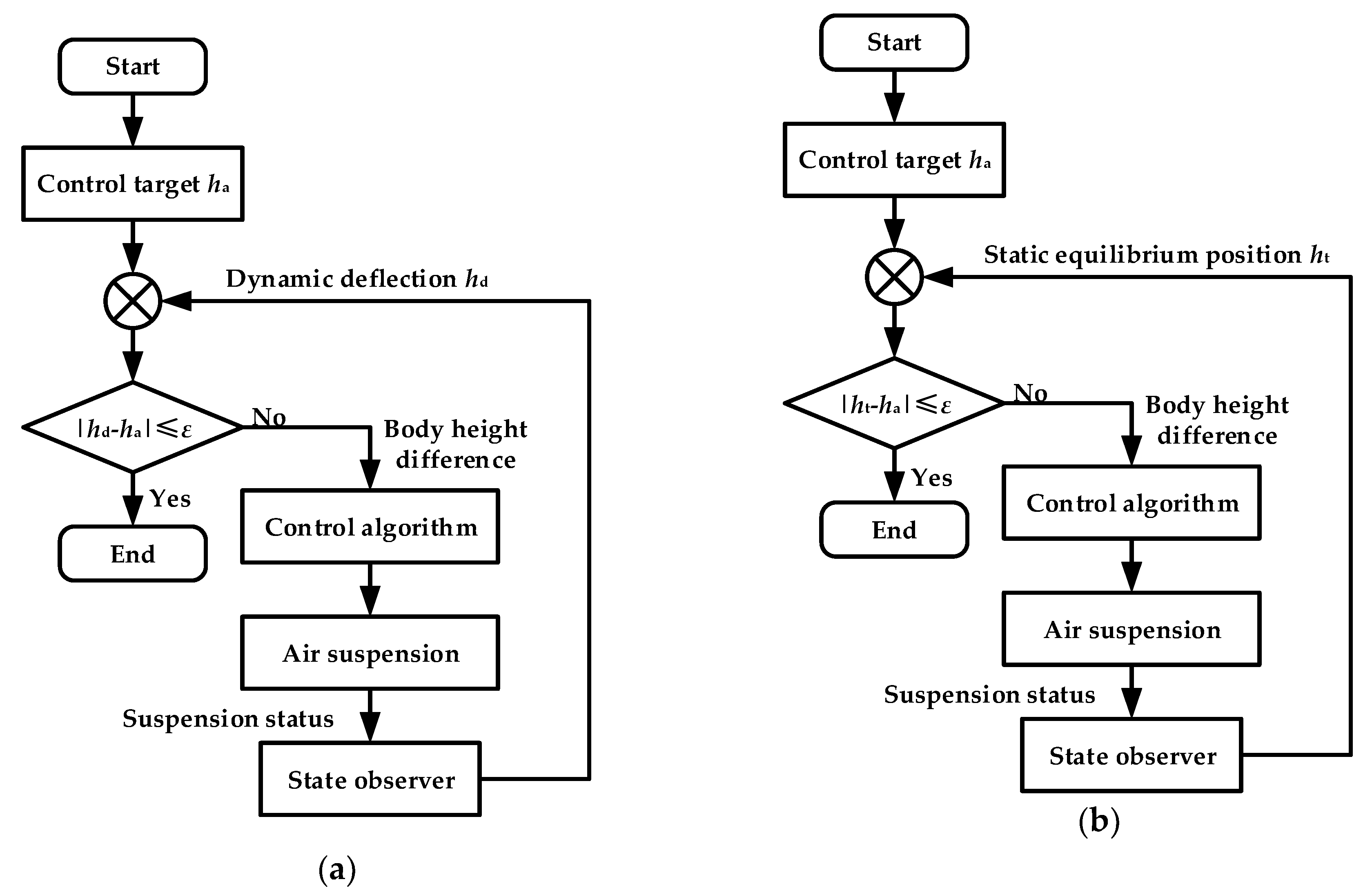
In general, actual vehicle height is compared with target height to determine whether the vehicle height has reacheed the target height. The control strategy selected in this paper is to use the static equilibrium position instead of suspension dynamic deflection as the adjustment basis. In order to verify the effectiveness of the control strategy, the dynamic deflection (as shown in Figure 4a) and the static equilibrium position (as shown in Figure 4b) are used to study the control effect. In the adjustment process, different target values are set according to different road conditions. The solenoid valve is closed when the static equilibrium position reaches the target value through the designed state observer. Subsequently, gas in the pneumatic spring will gradually reach steady state, such as curve A in Figure 5. Otherwise, there will be undesirable phenomena, such as repeated adjustment of height and over-inflating/over-deflating phenomena, which are shown as curve B in Figure 5.
3.1. The Establishment of State Observer
The vehicle observation algorithm is designed to observe the static equilibrium positions. Vertical velocity of vehicle body centroid , pitch angle change rate , roll angle change rate , vertical velocity of unsprung mass zwi, the suspension dynamic deflection zbi-zwi, the deformation of tire zwi-zgi, the suspension static equilibrium position hi and pressure inside the pneumatic chamber Pi are selected as the measurement variables and state equation are established as follows:
and the outputs are selected as follows:
The state equation of ECAS system is depicted as follows:
where:
with w is process excitation noise, ; v is process observation noise.
The time step is ∆T = 0.01 and the discretization of Equation (21) can be obtained as follows:
3.2. Unscented Kalman Filter Algorithm
The Kalman filter algorithm generally uses feedback control to estimate process states [35]. The ECAS system is a nonlinear system, hence suitable for the extended Kalman filter (EKF) algorithm and unscented Kalman filter (UKF) algorithm. However, EKF only retains the first order approximation, which leads to the generation of linear errors [36]. Moreover, the EKF relies on the derivation of the Jacobian matrix, so it requires a continuous adjustable state function and measurement function. However, UKF relies on the unscented transformation (UT), which avoids the tedious process of Jacobian matrix derivation and equations are not linearized using this algorithm, which can effectively improve the calculation accuracy [37]. The process of UT is as follows: the sampling points are substituted into nonlinear functions of the system, whose mean and variance are equal to the original state distribution. The transformed sample points are used to represent the probability density function of the Gauss density approximate state, so that the sample parameters have at least second-order accuracy. The Sigma transform is frequently used for UT. Suppose there is a nonlinear system y = f (x), the dimension of the state vector x is v. The mean and variance of points in the state distribution are and P, respectively. The Sigma points X and the relevant weight ω can be obtained by the following Equations (28) and (29), respectively:
where, m denotes mean; c denotes variance; λ is scaling factor; α stands for the distribution state of sampling points; β denotes nonnegative weight coefficient.
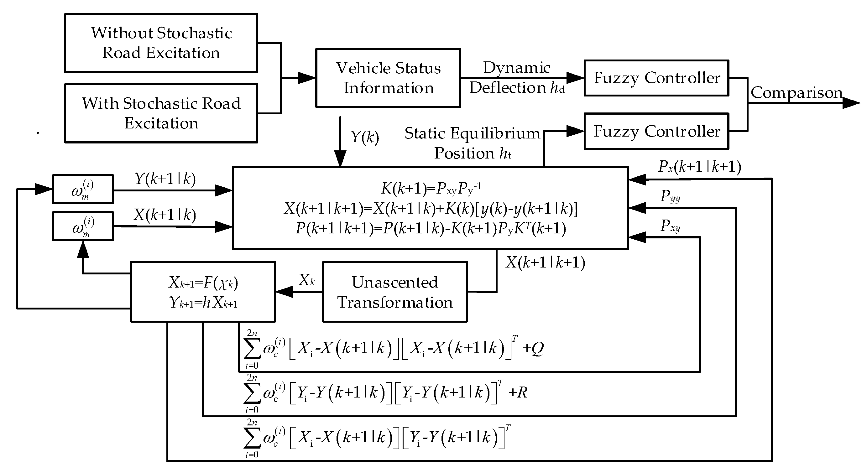
The UKF iteration is carried out using discretization Equations (25)–(27) and this specific process is shown in Figure 6. Using iterative results, suspension deflection and static equilibrium position can be used to adjust vehicle height, so as to compare control effect of different control strategies.
3.3. Fuzzy Controller
Since the solenoid valve used in the experiment is a switch solenoid valve, it has only two states of open and closed. The use of the fuzzy controller to output PWM can quickly control the switch of the solenoid valve and reduce the system delay so as to reduce the effect of the experimental environment on the experimental results to the maximum extent. At the same time, the rules of the fuzzy controller are easily modified and implemented. Moreover, the accuracy of the air suspension model does not need to be considered in the fuzzy controller and the adjustment process of suspension height can be optimized in real time. Therefore, a fuzzy controller is used to adjust the height of the vehicle.
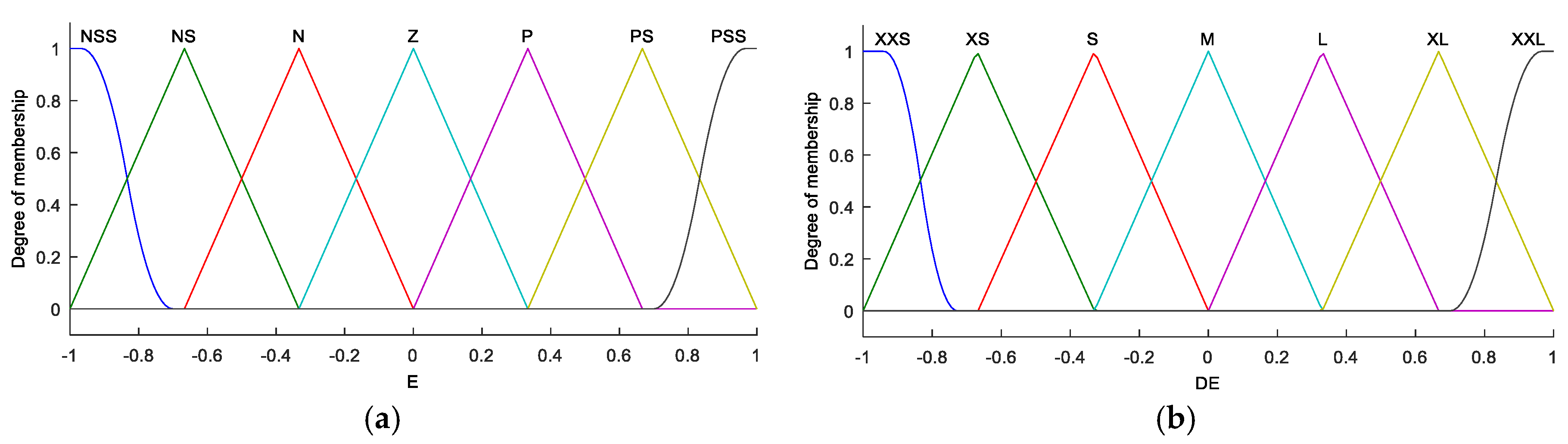
The height adjustment of the ECAS system is realized by using PWM to control the solenoid valve. In the process of adjustment, input variables are the difference e between the target height of vehicle and the static equilibrium position and variation rate de of the difference, respectively. The PWM duty cycle is used as the output variable u. Maximum change ranges of e, de and u can be obtained through system responses with external disturbances. The fuzzy rules need to be modified repeatedly according to the simulation results so as to get a good control effect. In order to ensure the accuracy of the adjustments, the change ranges of inputs and output should be divided into as many intervals as possible. In this paper, two input universes and an output universe of fuzzy controller are divided into seven ranges, as follows:
E = [ NSS NS N Z P PB PBB ]
DE = [ XXS XS S M L XL XXL ]
U = [ NNS NS S M B PB PPB ]
We set the membership function of input variables in Matlab/Simulink, as shown in Figure 7. On the basis of the fuzzy controller designed in this paper, a Mamdani algorithm is adopted in the inference engine and defuzzification is realized by using the centroid method.
According to the inputs and output, 49 linguistic rules of Fuzzy controller are formulated to achieve good control effect and its table is shown in Table 1.
4. Simulation
4.1. Paramaters of Model
The main parameters used in the model simulation are shown in Table 2.
4.2. Model Comparision
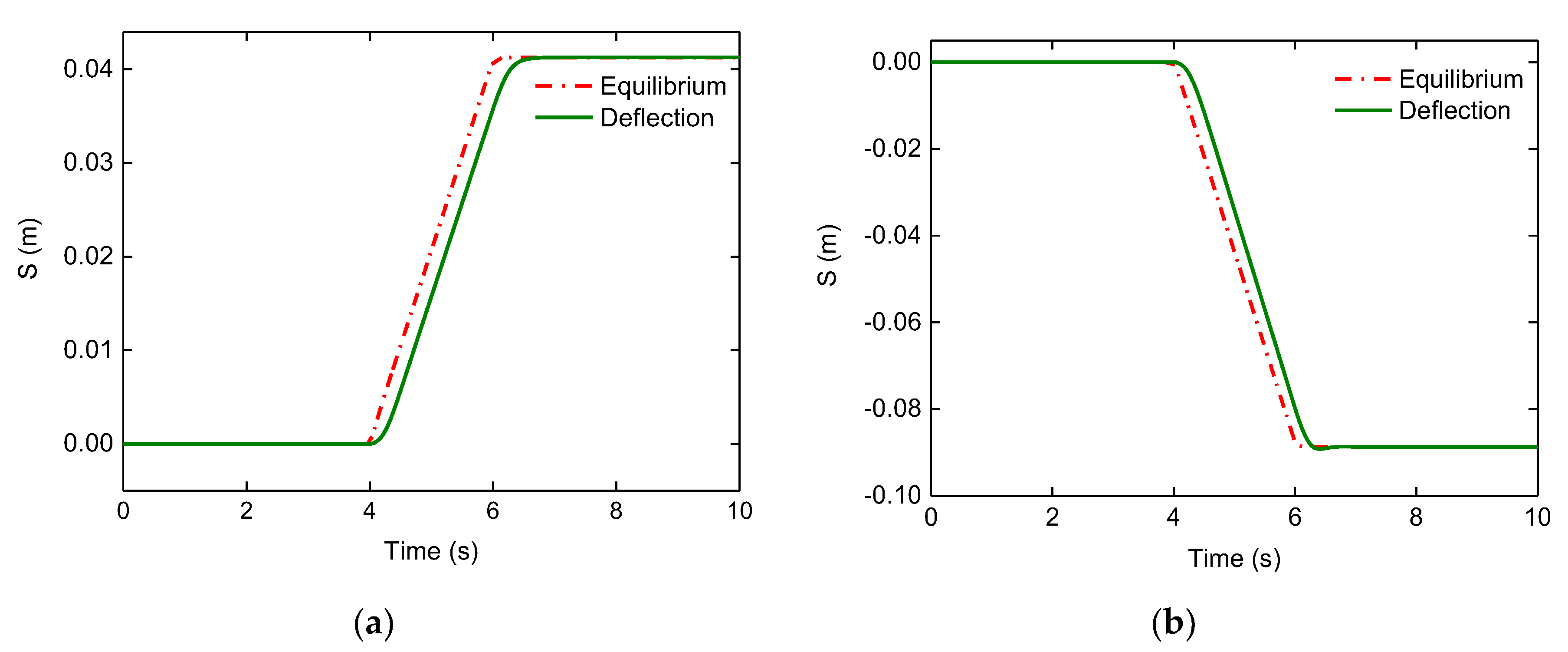
Before the model simulation, the suspension height and the static equilibrium position in the process of inflation/deflation are compared. Intake/exhaust solenoid valve is opened at 4 s and it is closed at 6 s. The response curves are shown in Figure 8.
According to the results, the length of the pipeline from the high pressure gas source to the pneumatic chamber is about 2 m and the length from the pneumatic chamber to the atmosphere is less than 0.5 m. Therefore, the rising height of the suspension is less than the lowering height, as shown in Figure 8. When the solenoid valve opens at 2 s, the suspension height begins to rise/decrease as the static equilibrium position rises/decreases. When the solenoid valve is closed at 6 s, the static equilibrium position observed by the state observer tends to be stable. The suspension height is basically consistent with the static equilibrium after a period of time due to the hysteresis of the inflating/deflating process. It is shown that the static equilibrium position is only related to the inflating/deflating process and its change can reflect the change of actual suspension height. Therefore, it can be used to control the suspension height and vehicle height.
4.3. Model Simulation
Simulation of the model is realized by the CarSim-AMESim-Simulink joint simulation platform. An air suspension model is developed in AMESim and parameters are transmitted into Matlab/Simulink through the S-Function. Parameters of the vehicle can be acquired by CarSim. The control strategy is designed and implemented in Matlab/Simulink. Based on the simulation results, curves are defined as follow: curve H-E denotes the curve of suspension height change adjusted by the static equilibrium position; curve H-D denotes the curve of suspension height change adjusted by the suspension deflection; curve C-E denotes the curve of vehicle centroid height change adjusted by the static equilibrium position; curve C-D denotes the curve of centroid height change adjusted by the suspension deflection.
4.3.1. Statics
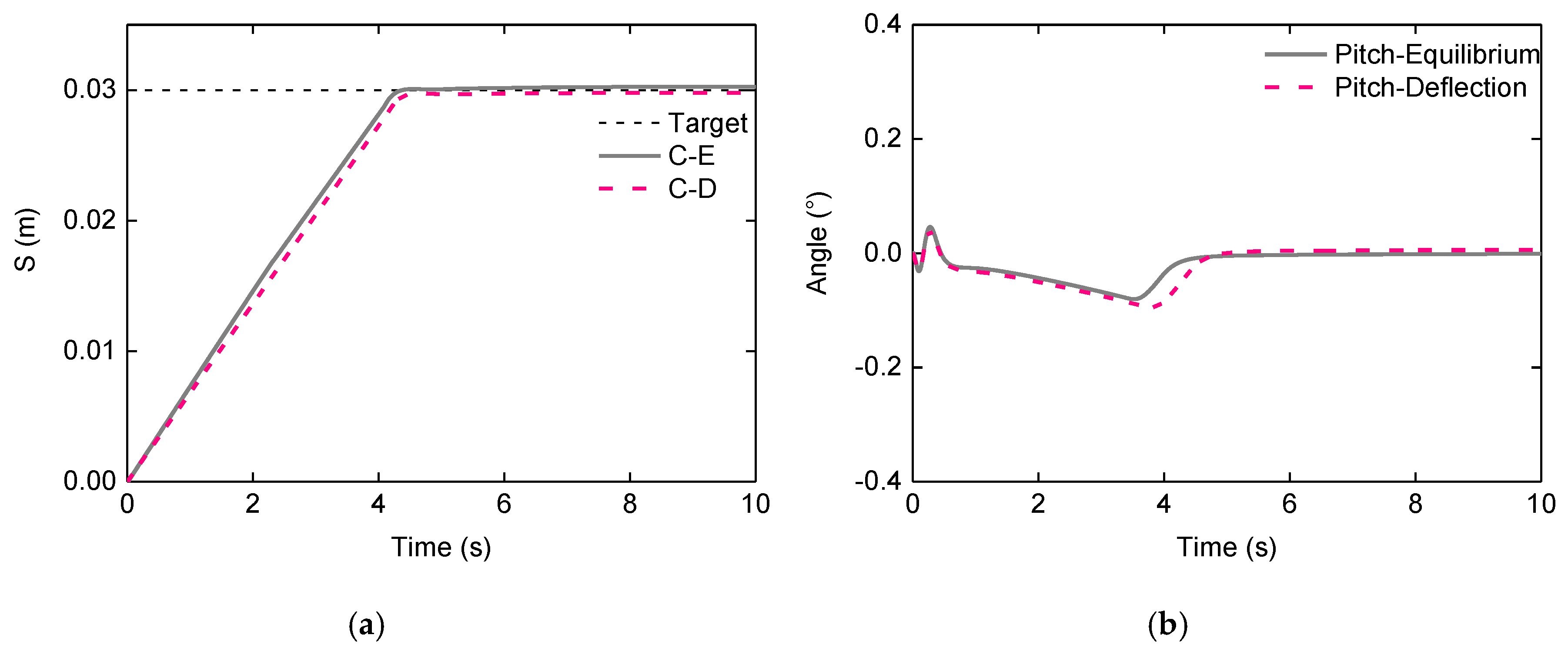
When the vehicle is stationary, the target height is set to ±0.03 m. To effectively reflect the system characteristics, height changes of the front left and rear left suspensions are displayed. Vehicle parameters are shown in Table 2 and response curves are shown in Figure 9, Figure 10, Figure 11 and Figure 12, respectively.
It can be seen from Figure 9, the height changes of the front left and rear left suspension adjusted by deflection are 0.02996 and 0.02995 m, respectively, and the control accuracy is above 99%. Height changes adjusted by the static equilibrium position are 0.03004 and 0.03001 m, respectively, and the control accuracy is above 99%. Because there is no road excitation, the suspension deflection can reflect suspension height changes. However, the static equilibrium position is only related to the process of inflation/deflation, so solenoid valves are closed after reaching the target position. According to Figure 10, the vehicle height changes based on suspension deflection and the static equilibrium position are 0.0305 and 0.0301 m, respectively, and the adjustment accuracy is over 99%. The error is less than the error given error in [22]. As the static equilibrium position is related to the on-off state of solenoid valve, maximum pitch angle is 0.08°, which is smaller than the 0.095° adjusted by the suspension deflection.
Similarly, the deflating process is shown in Figure 11 and Figure 12. The cross-sectional area of the exhaust valve is smaller than that of intake valve, so the adjustment time is slightly longer. As can be seen from Figure 11, the height changes of the front left and rear left suspensions adjusted by deflection are 0.02956 m and 0.02939 m, respectively, and the control accuracy is above 98%. The height changes adjusted by the static equilibrium position are 0.03026 m and 0.03001 m, respectively, and the control accuracy is also above 98%. According to Figure 12, the height changes of the vehicle centroid based on suspension deflection and the static equilibrium position are −0.03006 m and −0.03002 m, respectively. In the process of vehicle height lowering, the adjustment accuracy is over 99.6% and error is less than the error given in [22].
It’s known from the process of vehicle height lifting and lowering that the error of pitch angle is not more than 0.1° and this control algorithm can effectively ensure the stability of the vehicle attitude.
4.3.2. Speed Control Bump
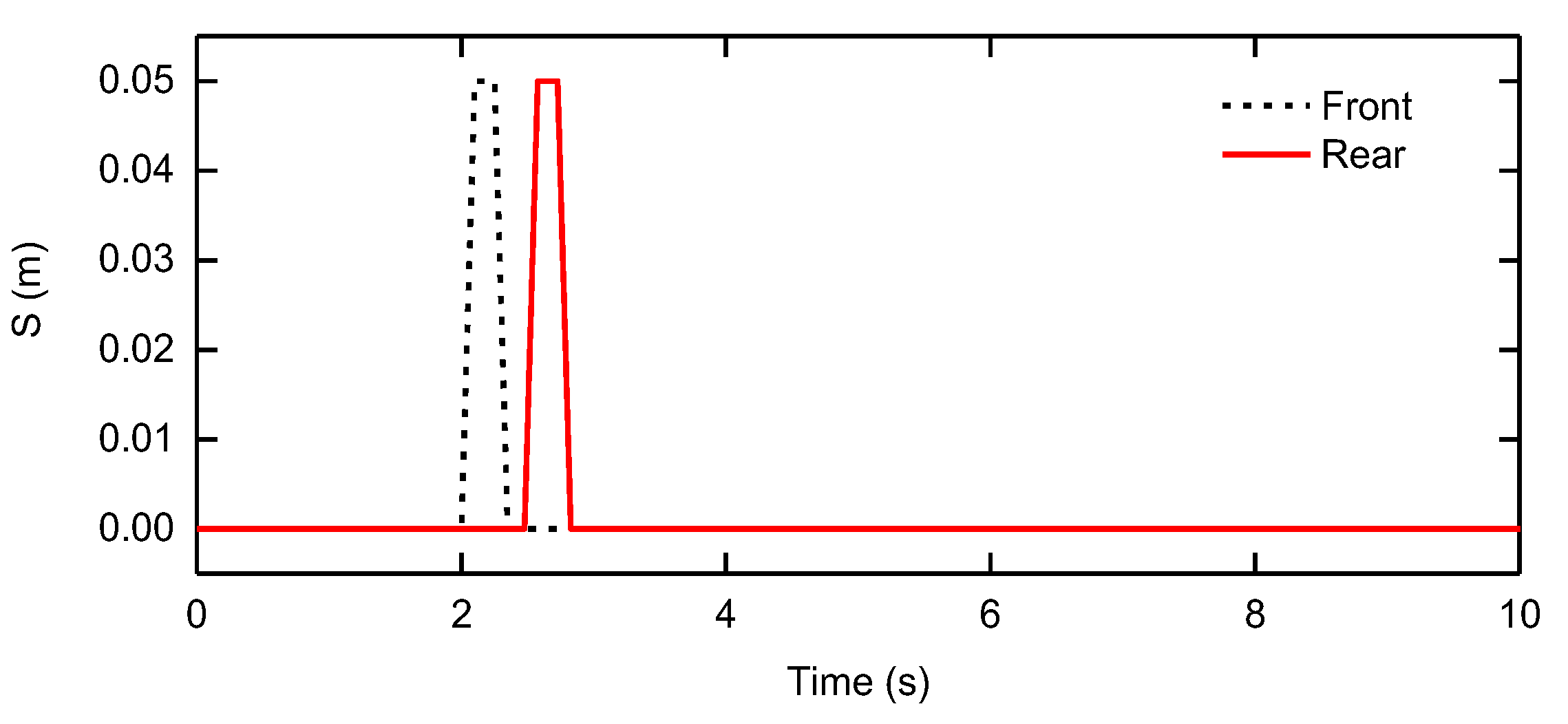
The vehicle speed is set to 20 km/h. Because of the influence of the vehicle wheelbase, there is a lag between the excitation signal of the rear axle and the front axis and the signal inputs of the speed control bump are shown in Figure 13. The vehicle target height is set to 0.03 m and the rising process is disturbed by the speed control hump at 2 s. The response curves of system parameters are shown in Figure 14 and Figure 15.
It is found from Figure 14 that the suspension deflection varies greatly at 2 s. The suspension height changes adjusted by dynamic deflection are as follows: 0.02257, 0.0239, 0.02014 and 0.02133 m. Suspension height changes adjusted by the static equilibrium position are as follows: 0.02995, 0.02994, 0.02998 and 0.02997 m. It can be seen that maximum error adjusted by dynamic deflection is over 0.006 m, which deviates from the target height. Furthermore, the height change of the vehicle centroid is 0.02399 m and it doesn’t reach the desired height, as seen in Figure 15a. However, because the static equilibrium position of the air suspension has strong robustness, it’s not disturbed by the road excitation. Therefore, when it is used to adjust suspension height, the effect of the excitation signal is very small. The control accuracy is over 97%, which meets the actual requirement. The height change of the vehicle centroid is 0.0305 m and its control accuracy can reach over 98.3%. Due to the interference of the speed control bump, the pitch angle is 0.05° and vehicle produces a pitch motion after the height is adjusted according to the suspension dynamic deflection. On the contrary, the vehicle body adjusted according to the static equilibrium position will gradually converge to a stationary state after passing over the speed bump. Therefore, the vehicle body posture adjusted by the static equilibrium position is more stable.
4.3.3. B Level Typical with Speed 90 km/h
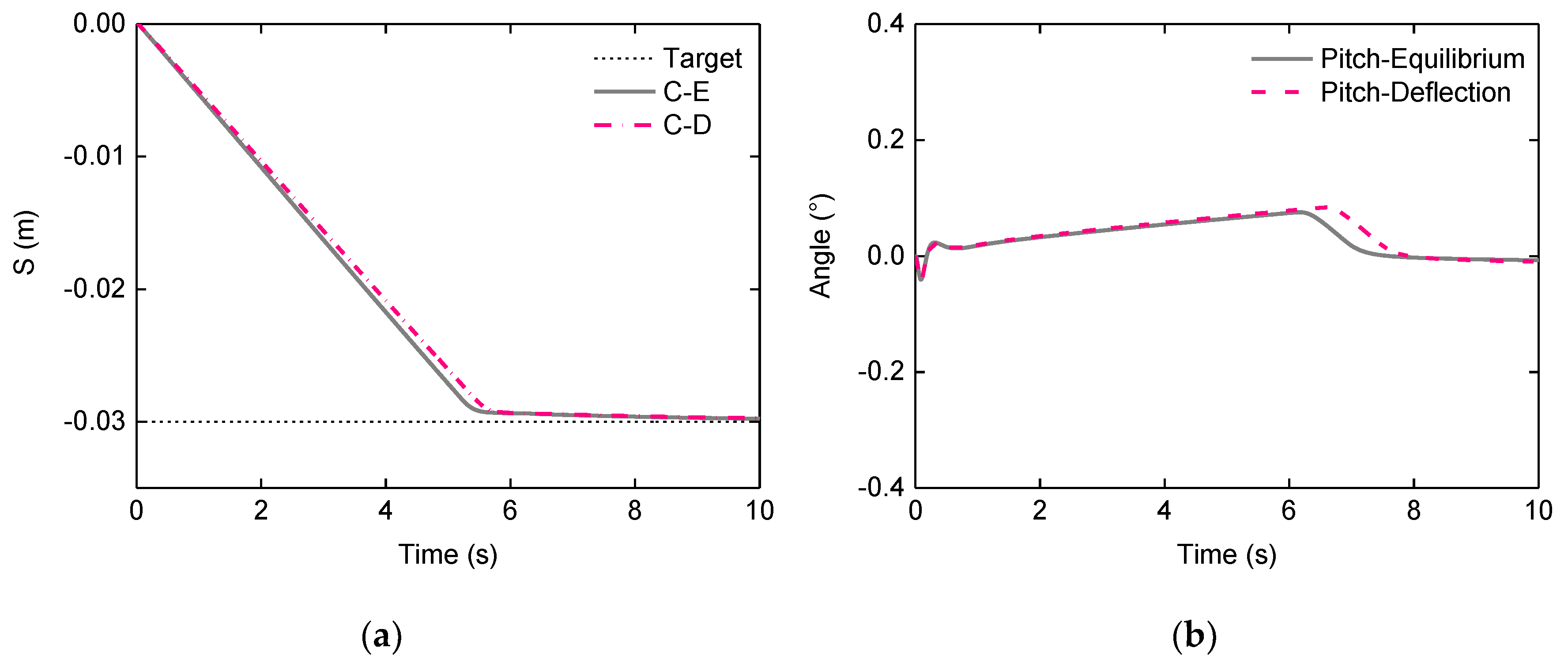
When the vehicle is running at 90 km/h speed on a B level typical road, it’s necessary to reduce the vehicle height in order to improve handling stability and reduce the air resistance so as to extend its mileage. Therefore, the ECU needs to send control commands to the actuator and the system enters into economy mode. Target height is set to −0.03 m and the response curves are shown in Figure 16 and Figure 17.
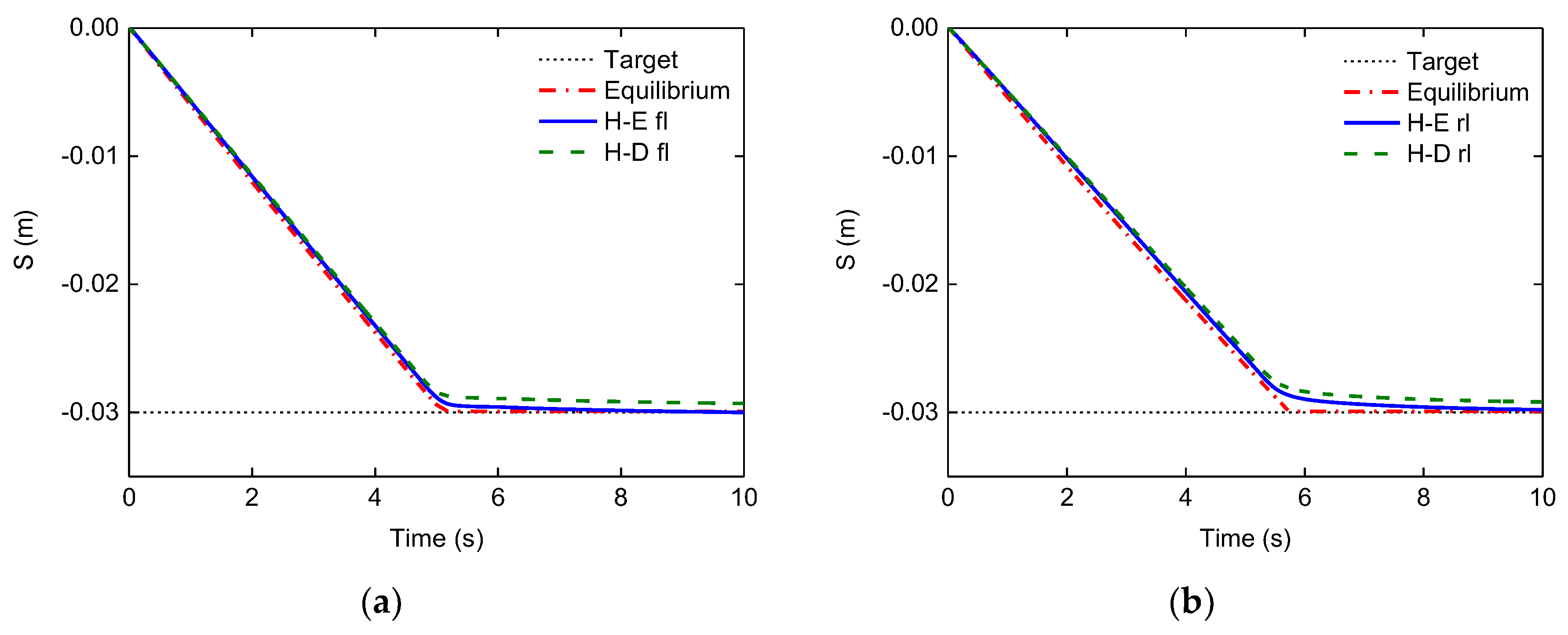
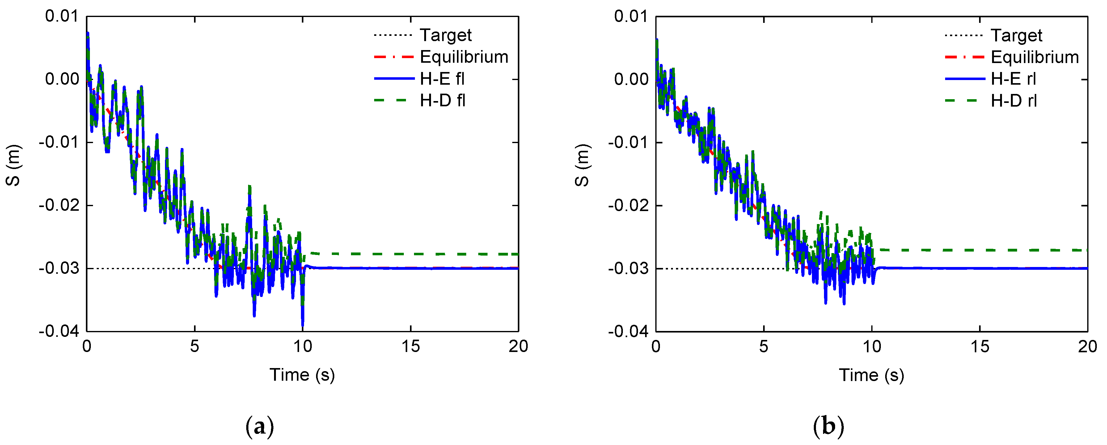
The suspension dynamic deflection can’t accurately indicate the actual suspension height change because it varies with road irregularities. It can be seen from Figure 16 that the height changes of the front left suspension and rear left suspension adjusted by dynamic deflection are −0.02774 m and −0.02703 m, respectively, and the control accuracy is lower than 93%. Height changes adjusted by the static equilibrium position are 0.03001 m and 0.02993 m, respectively, and the control accuracy is also above 99%. Therefore, the suspension height adjusted by dynamic deflection is far from the target height of −0.03 m, which does not meet the precision requirements. The height change of the vehicle centroid adjusted by dynamic deflection is 0.0282 m obtained from Figure 17, which doesn’t reach the desired height.
The above simulation results show the failure of the control strategy based on the suspension dynamic deflection. However, the static equilibrium position is not affected by the road excitation. Accordingly, the static equilibrium position can ensure that the solenoid valve is closed when the suspension height reaches the ideal height and it simultaneously has a stronger robustness, as seen in Figure 16. From Figure 17, it’s known that the height change of vehicle centroid is 0.03035 m and its accuracy is above 98%. Furthermore, the pitch angle and roll angle are 0.00008° and 0.00048° respectively, which can be effectively controlled by adjusting the suspension height so as to better ensure the stability of the vehicle body attitude.
5. Experiments
The components used in a realistic vehicle experiment are shown in Figure 18. The air pump is controlled by the ECU. There are two CAN buses for communication in the ECAS system. CAN1 bus is used to realize the communication between the control box and the system, and the CAN0 bus is used to download control programs into the ECU, collect height and pressure signals and communicate with the ECU to control the solenoid valves. The baud rate of CAN bus communication is set to 500 kbits/s and the cycle period of program is 20 ms. At the same time, the height signals and pressure signals of vehicle are also collected and analysed through DEWESoft X2.
5.1. Model Verification
Before the start of the experiment, the air suspension model, 7-DOF vehicle model and UKF algorithm need to be verified. The air suspension model is verified based on the bench test and other verifications are based on real vehicle tests.
5.1.1. Air Suspension Model Verification
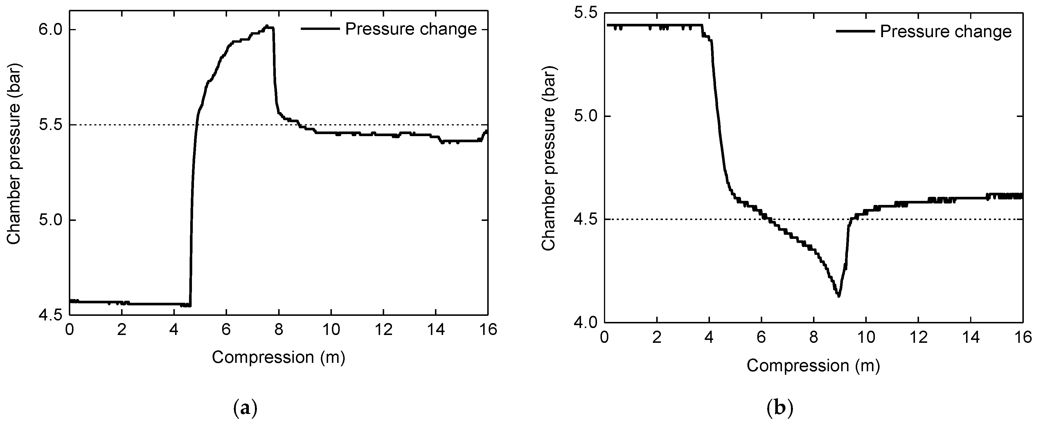
Firstly, the air suspension on the vehicle is tested by bench tests and its characteristic stiffness curve is shown in Figure 19. This curve shows the relationship between the pressure in pneumatic chamber and the suspension height change. The initial absolute pressure of the air suspension is set to 4.54 bar and the suspension height is in the lowest position. Because the travel L of the air suspension is −60–50 mm, air suspension is inflated to increase 110 mm. It can be obtained through the bench tests that the pressure in air suspension is 5.423 bar when the height of the air suspension increases 0.04 m.
Simulation in AMESim using the air suspension parameters was used in the vehicle experiments. When the suspension height increases 0.04 m from the lowest position, the pressure changes are as shown in Figure 20a. As one can see from Figure 20a, the initial absolute pressure is 4.57 bar without inflating and the gas pressure is 5.42 bar when the suspension height increases 0.04 m. The simulation is in agreement with the experimental results. Although the instantaneous gas pressure is up to 6.0 bar and in the process of inflating it takes slightly longer, this is only the excess pressure of the local gas and the pressure is restored to 5.42 bar after the gas reaches the equilibrium state. When the suspension height reduces 0.04 m, the pressure changes as shown in Figure 20b. The initial absolute pressure is 5.441 bar and the gas pressure is 4.62 bar when the deflating process has ended. The simulation results show that model can effectively reflect the stiffness characteristics of the air suspension, so this model is used in the simulation.
5.1.2. 7-DOF Vehicle Model Verification
7-DOF vehicle model is verified by its centroid position. The centroid position of the vehicle body in the simulation can be easily obtained, but in the experimental process, it needs to be calculated by the change of suspension height, pitch angle and roll angle. Pitch angle and roll angle can be obtained by a gyroscope. The simulation model is verified by comparison of the different centroid positions. When the vehicle is stationary, the heights of the front left and front right suspensions increase 0.04 m, respectively. The displacement of the vehicle centroid is calculated using the collected signals, which are then compared with the simulation results. Similarly, the heights of front left and rear left suspensions increase 0.04 m, respectively. The correctness and accuracy of the 7-DOF model are verified by the experiments described above. The simulation and experimental results are compared, as shown in Figure 21.
In Figure 21a, the experimental result is 0.59506 m and the simulation result is 0.59399 m. The error is 0.00107 m. In Figure 21b, the experimental result is 0.59661 m and the simulation result is 0.59609 m. The error is 0.00052 m. The errors of the experimental results may come from the uneven load of the actual vehicle and the loss of gas in the pipeline. The error rate is less than 1%, so the error is within the allowable range. This shows that the simulation results are basically consistent with the centroid position of the vehicle calculated according to an actual vehicle. Therefore, in the process of vehicle height adjustment, the centroid height of the vehicle is chosen as the basis for judging the stability of the vehicle body attitude.
5.1.3. UKF Algorithm Verification
When the vehicle is running on the road, the vehicle height is adjusted. After a certain distance, the height changes of the dynamic deflection and the static equilibrium position are compared. Height and pressure signals are used by the UKF algorithm. We control the solenoid valves to inflate and deflate the pneumatic chamber for a period of time, respectively. At 12 s, the vehicle stops driving. The changes of vehicle suspension and the static equilibrium position of the front-left wheel are shown in Figure 22, where it can be seen from Figure 22a that when the vehicle is driving, the error between dynamic deflection and the static equilibrium position is caused by the road excitation. When the vehicle stops, the height changes of the static equilibrium position obtained are 0.32365 m and 0.25028 m, respectively. The deflection changes are 0.32341 m and 0.25034 m, respectively. The errors between the dynamic deflection and the static equilibrium position are 0.00024 m and 0.00006 m, respectively, and the accuracy of model is over 99%. It can also be seen that from the closing time of the solenoid valve to 12 s, the maximum error range between the dynamic deflection and the static equilibrium position is 0.00667 mm. Then, the dynamic deflection reduces 0.002 m at 12 s and it’s explained that the dynamic deflection does not correctly reflect the vehicle height change because of the effect of road excitation.
When the solenoid valve is closed, there is an overshoot phenomenon in the adjustment process of the static equilibrium position. Because it is related to pressure in the pipeline, the sudden closure of a solenoid valve will cause an excessive local pressure and the overshoot phenomenon occurs, but the pressure of a small amount of high pressure gas gradually reaches stability. When the solenoid valve is just closed, the errors between the static equilibrium position and the suspension height are 0.00832 m and −0.0055 m, respectively. When the vehicle stops and the gas is completely stable, the static equilibrium position is basically the same as the suspension height and is in line with the desired accuracy.
5.2. Experimental Verification
Because the 7-DOF vehicle model has been verified by a real vehicle, the centroid position of the vehicle can be used as a reference for the vehicle height adjustment. According to the suspension height adjusted by dynamic deflection and the static equilibrium position, the corresponding centroid height can be obtained. All the experiments are carried out in a real vehicle.
5.2.1. Vehicle Is Static
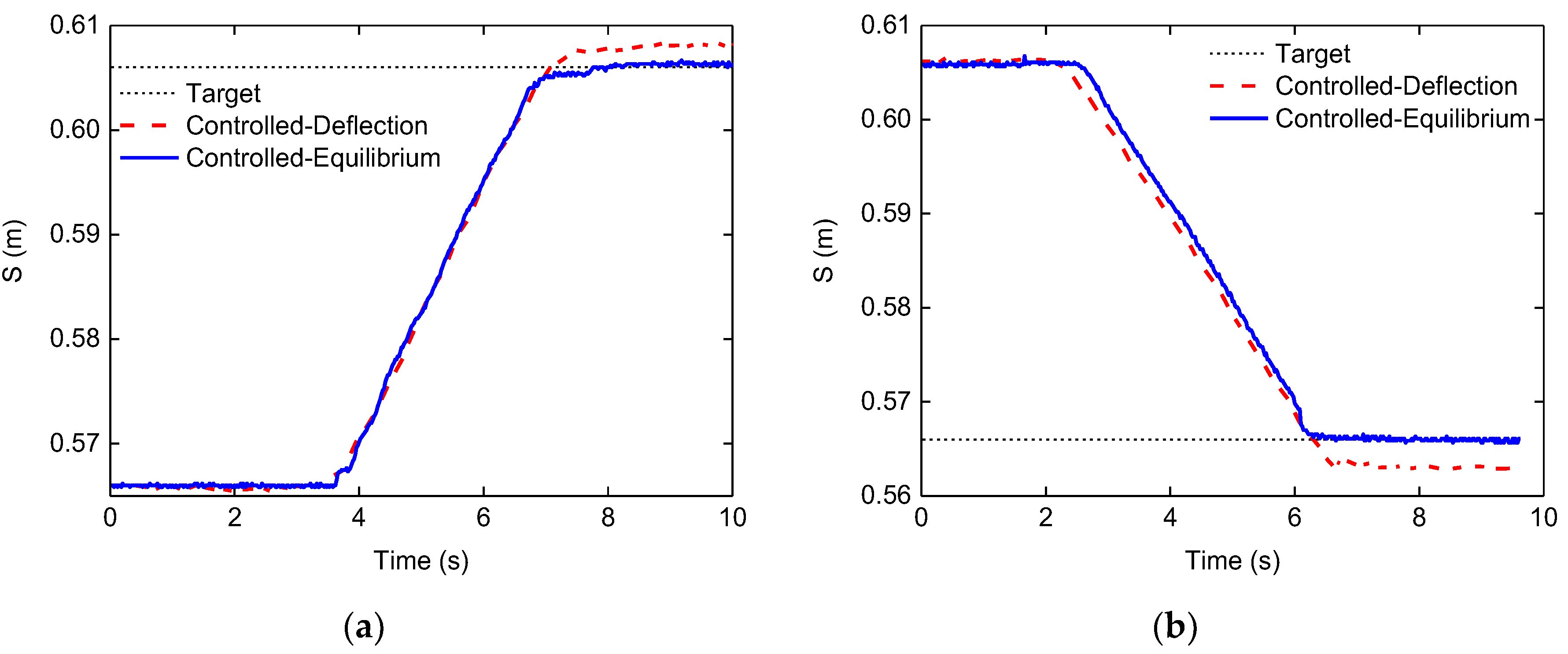
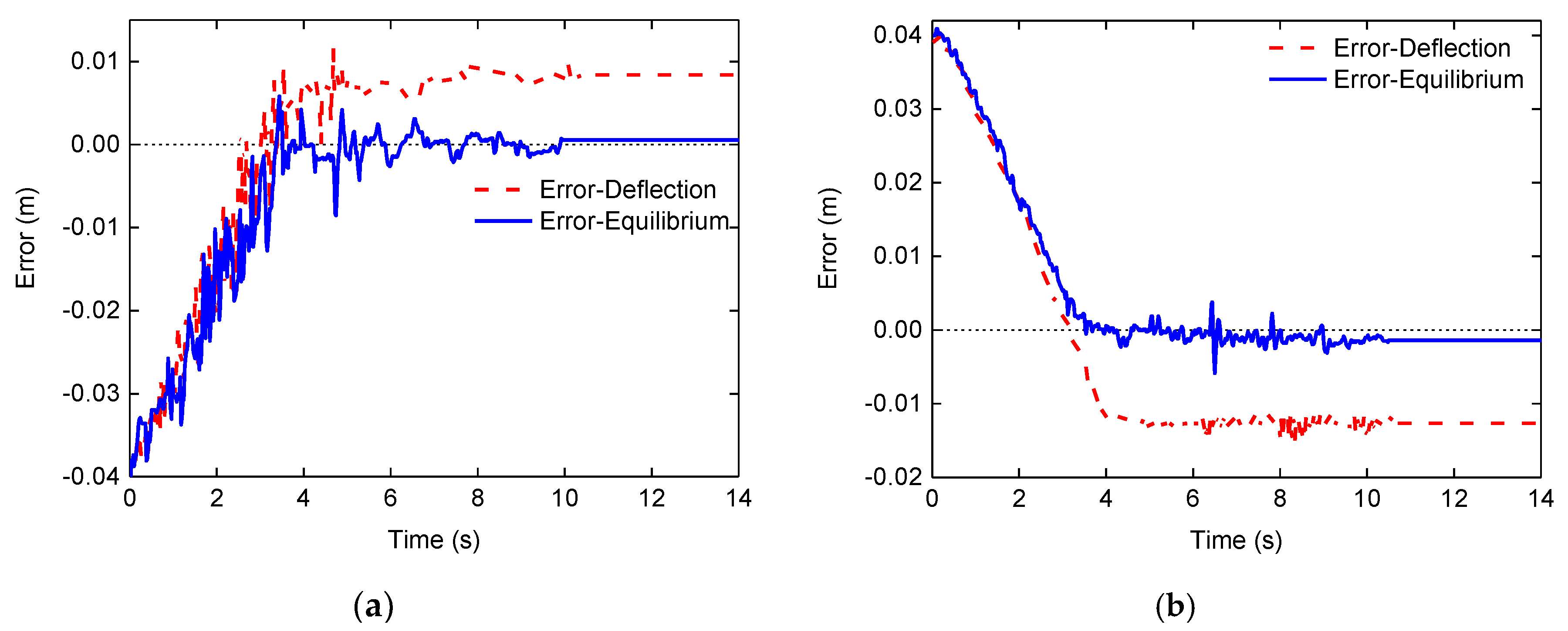
When the vehicle is static, the target height is set at ±0.04 m, respectively. During the process of inflating and deflating, the target heights of the centroid are set as 0.606 m and 0.566 m, respectively. Height changes of the vehicle centroid without stochastic road excitation are shown in Figure 23 and height errors are shown in Figure 24. After the inflating process, the centroid height adjusted according to suspension deflection and the static equilibrium position are 0.60877 m and 0.60617 m, respectively, as seen in Figure 23a. It can be seen from Figure 24a that the maximal height error of centroid position adjusted by deflection is up to 0.00277 m. When the deflection reaches the target height, the ECU sends instructions to close the solenoid valve. Because of the existence of hysteresis in the system, the excess gas comes into the pneumatic chamber and an overshoot phenomenon occurs, as shown in Figure 23a. However, the maximal height error of the centroid position adjusted by the static equilibrium position is 0.00017 m and the error 0.425%. When the calculated static equilibrium position reaches the desired target height, the solenoid valve is immediately closed and there will be little gas coming into the pneumatic chamber so that overshoot phenomenon can be effectively eliminated. Similarly, after the deflating process, the centroid height adjusted by suspension deflection and the static equilibrium position are 0.56292 m and 0.56609 m, respectively, as seen in Figure 24b. The maximal height error is up to 0.00308 m. The maximal height error adjusted by the static equilibrium position is up to 0.00009 m. In the process of inflating and deflating, the adjustment accuracy of centroid height adjusted by the static equilibrium position is more than 99%. Therefore, the adjustment accuracy of the static equilibrium position satisfies our needs. After the solenoid valve is closed, the static equilibrium position gradually reaches the target height and the human body will be unable to perceive the resulting tiny vibrations which can be ignored.
5.2.2. Vehicle Is Running on the Road
When the vehicle is running on a poor road, the vehicle body vibration is strong and the vehicle height increases 0.04 m, as seen in Figure 25a; while when the vehicle is running on a good road, the handling stability of the vehicle is particularly important and the vehicle height needs to reduce 0.04 m, as seen in Figure 25b. In these processes, the target heights of the centroid are set to 0.606 m and 0.566 m, respectively. The vehicle begins to decelerate from the 5 s point and vehicle has completely stopped at 10 s.
In the process of inflating, it can be known from Figure 25a that the centroid height adjusted by dynamic deflection exceeds the target height. When the vehicle stops, the centroid height is 0.61448 m. The error is 0.00848 m and far beyond the desired height. However, the centroid height adjusted by the static equilibrium position is 0.60654 m and its error is 0.00054 m, as seen in Figure 26a. Experimental results show that vehicle height adjustment accuracy according to the static equilibrium position is more than 97%. In the process of deflating, it can be known from Figure 25b that when vehicle stops, the centroid height is 0.55448 m. The error is 0.01152 m and also far beyond the desired height.
However, the centroid height adjusted by the static equilibrium position is 0.565 m and error is 0.001 m, as seen in Figure 26b. The experimental results show that dynamic adjustment accuracy of vehicle height is more than 98% according to the static equilibrium position. According to the experimental results, the static equilibrium position of suspension can not only realize static vehicle height adjustment, but also avoid the disturbance caused by road excitation during the vehicle driving process. The experimental results show that control strategy has good adaptability for different road conditions. The results illustrate that this proposed control strategy can meet the requirements.
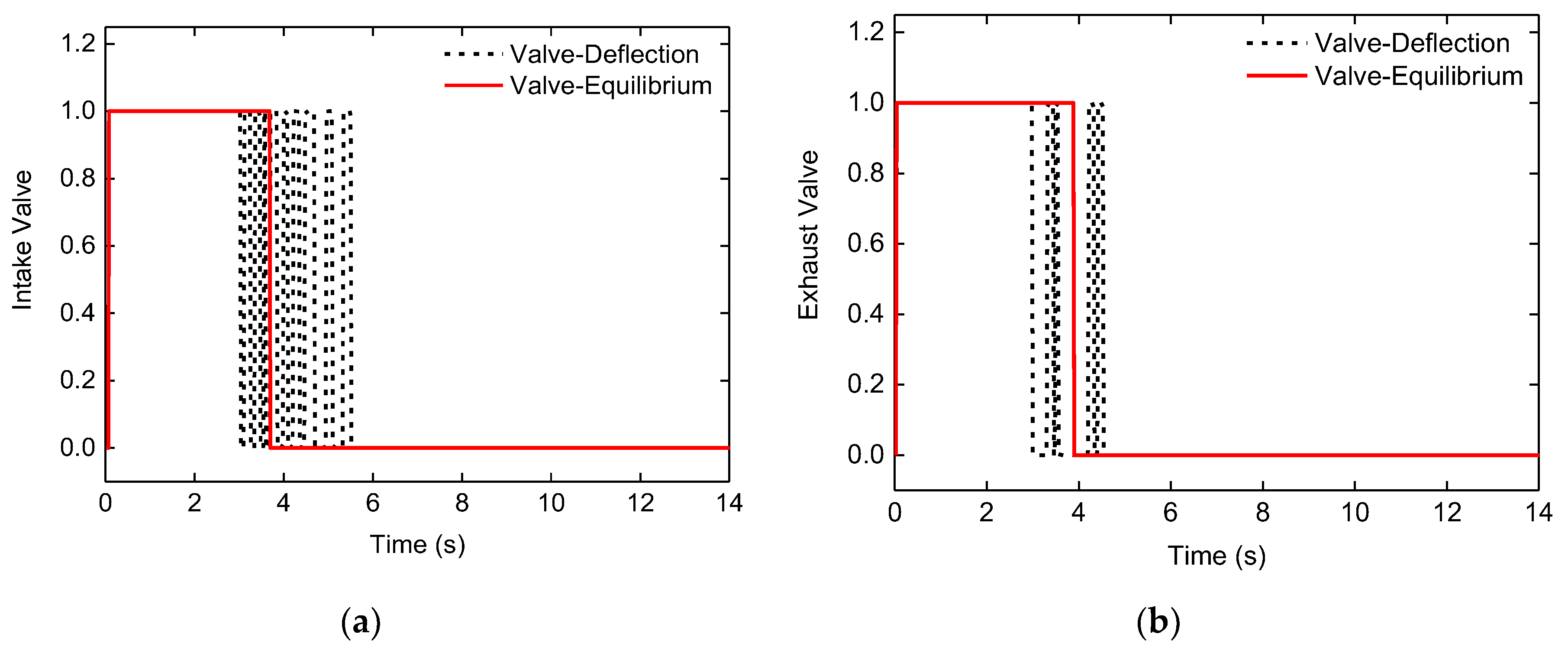
Furthermore, frequent switching of the solenoid valve will be caused by road excitation when the vehicle height, which is adjusted by suspension dynamic deflection, is close to the target height, as shown at 3–6 s in Figure 27a and 3–5 s in Figure 27b. Meanwhile, we can know that when the road excitation is strong, the state of the solenoid valve changes more brusquely by comparing Figure 27a,b. This will seriously affect the stability and life of the ECAS system. Conversely, the static equilibrium position is not related to road excitation, so the solenoid valve will be closed only after the height reaches the target height. This is of great significance to reduce the noise disturbance, keep the system stable and prolong the life of the system.
6. Conclusions
In this paper, a vehicle height adjustment algorithm based on the static equilibrium position of air suspension is proposed according to the gas flow characteristics of the air suspension in the process of inflating/deflating. The static equilibrium position is obtained using the unscented Kalman state observer. On this basis, a fuzzy controller is designed to realize height adjustment of the vehicle.
The simulation results show that suspension height adjustment based on the static equilibrium position not only improves the accuracy of vehicle height adjustment in the static state, but also the control precision of the vehicle height and the stability of the vehicle attitude is ensured when road surface excitation is present.
From the analysis of the experimental results, we can see that the application of the static equilibrium position can achieve accurate adjustment of the vehicle height under various complex road conditions, so as to ensure that the vehicle displays a comprehensive positive driving performance experience.
Acknowledgments
This is supported by the National Nature Science Foundation of China (grant number 51375046 and 51205021).
Author Contributions
Zepeng Gao and Yuzhuang Zhao conceived original ideas; Zepeng Gao, Yuzhuang Zhao and Sizhong Chen performed the simulations and designed the experiment; Zepeng Gao, Yuzhuang Zhao, Sizhong Chen and Jinrui Nan wrote the manuscript; Yuzhuang Zhao directed the overall project. All authors analyzed the data and discussed the results and comments on the manuscript.
Conflicts of Interest
The authors declare no conflict of interest.
References
- Xiong, R.; Tian, J.P.; Mu, H.; Wang, C. A systematic model-based degradation behavior recognition and health monitor method of lithium-ion batteries. Appl. Energy 2017, 207, 367–378. [Google Scholar] [CrossRef]
- Yu, Q.; Xiong, R.; Lin, C.; Shen, W.X.; Deng, J.J. Lithium-ion Battery Parameters and State-of-Charge Joint Estimation Based on H infinity and Unscented Kalman Filters. IEEE Trans. Veh. Technol. 2017, 66, 8693–8701. [Google Scholar] [CrossRef]
- Chen, C.; Xiong, R.; Shen, W. A lithium-ion battery-in-the-loop approach to test and validate multi-scale dual H infinity filters for state of charge and capacity estimation. IEEE Trans. Power Electron. 2018, 33, 332–342. [Google Scholar] [CrossRef]
- Xiong, R.; Cao, J.Y.; Yu, Q.; He, H.; Sun, F.C. Critical review on the battery state of charge estimation methods for electric vehicles. IEEE Access 2017, 6, 1832–1843. [Google Scholar] [CrossRef]
- Woodrooffe, J. Heavy Truck Suspension Dynamics: Methods for Evaluating Suspension Road Friendliness and Ride Quality; SAE: Warrendale, PA, USA, 1996. [Google Scholar] [CrossRef]
- Bao, W.; Chen, L.P.; Zhang, Y.Q. Fuzzy Adaptive sliding mode controller for an air spring active suspension. Int. J. Automot. Technol. 2012, 13, 1057–1065. [Google Scholar] [CrossRef]
- Niea, S.; Zhuang, Y.; Liu, W.; Chen, W. A Semi-active suspension control algorithm for vehicle comprehensive vertical dynamics performance. Veh. Syst. Dyn. 2017, 55, 1099–1122. [Google Scholar] [CrossRef]
- Schonfeld, K.; Geiger, H.; Hesse, K. Electronically Controlled Air Suspension (ECAS) for Commercial Vehicles; SAE: Warrendale, PA, USA, 1991. [Google Scholar] [CrossRef]
- Nagai, M.; Moran, A.; Tamura, Y.; Koizumi, S. Identification and control of non-linear active pneumatic suspension for rail way vehicles using neural networks. Control Eng. Pract. 1997, 5, 1137–1144. [Google Scholar] [CrossRef]
- Meller, T. Self-Energizing Leveling Systems Their Progress in Development and Application; SAE: Warrendale, PA, USA, 1999; pp. 42–45. [Google Scholar]
- Chen, Y.; Chen, L.; Wang, R.; Xu, X.; Shen, Y.; Liu, Y. Modeling and test on height adjustment system of electrically-controlled air suspension for agricultural vehicles. Int. J. Agric. Biol. Eng. 2016, 9, 40–47. [Google Scholar]
- Kyuhyun, S.; Lee, H.; Ji, W.; Choi, C.; Hwang, S. Effectiveness evaluation of Hydro-Pneumatic and Semi-active Cab suspension for the Improvement of ride comfort of agricultural tractors. J. Terramech. 2017, 69, 23–32. [Google Scholar]
- Sayyaadi, H.; Shokouhi, N. New dynamics model for rail vehicles and optimizing air suspension parameters using GA. Sci. Iran. 2009, 16, 496–512. [Google Scholar]
- Alonso, A.; Giménez, J.G.; Vinolas, J. Air suspension characterisation and effectiveness of a Variable Area Orifice. Veh. Syst. Dyn. 2010, 48, 271–286. [Google Scholar] [CrossRef]
- Nakajima, T.; Shimokawa, Y.; Mizuno, M. Air suspension system model coupled with leveling and differential pressure valves for railroad vehicle dynamics simulation. J. Comput. Nonlinear Dyn. 2014, 9, 149–155. [Google Scholar] [CrossRef]
- Löcken, F.; Welsch, M. The dynamic characteristic and hysteresis effect of an Air Spring. Int. J. Appl. Mech. Eng. 2015, 20, 127–145. [Google Scholar] [CrossRef]
- Zhu, H.; Yang, J.; Zhang, Y.; Feng, X. A novel Air Spring Dynamic Model with Pneumatic Thermodynamics, Effective Friction and Viscoelastic Damping. J. Sound Vib. 2017, 408, 87–104. [Google Scholar] [CrossRef]
- Such, Y.; Kumaki, S. Study on curving characteristic of enhance vehicle stability. Int. J. Veh. Des. 2000, 23, 124–144. [Google Scholar]
- Lee, I.; Park, J.; Shin, M.; Jang, J. Study of failure examples of automotive electronic control suspension system including cases with wiring disconnection and air leakage. J. Korean Soc. Tribol. Lubr. Eng. 2013, 29, 180–185. [Google Scholar] [CrossRef]
- Prabu, K.; Jancirani, J.; John, D. Vibration control of air suspension system using PID controller. J. Vibroeng. 2013, 15, 132–138. [Google Scholar]
- Xiong, R.; Yu, Q.; Wang, L.Y.; Lin, C. A novel method to obtain the open circuit voltage for the state of charge of lithium ion batteries in electric vehicles by using H infinity filter. Appl. Energy 2017, 207, 341–348. [Google Scholar] [CrossRef]
- Xu, X.; Chen, L.; Sun, L.; Sun, X. Dynamic ride height adjusting controller of ECAS vehicle with random road disturbances. Math Probl. Eng. 2013, 2013. [Google Scholar] [CrossRef]
- Xu, X.; Zhou, K.; Zou, N.; Jiang, H.; Cui, X. Hierarchical control of ride height system for electronically controlled air suspension based on variable structure and fuzzy control theory. Chin. J. Mech. Eng. 2015, 28, 945–953. [Google Scholar] [CrossRef]
- Sun, X.; Chen, L.; Wang, S.; Xu, X. Vehicle height control of electronic air suspension system based on mixed logical dynamical modelling. Sci. China Technol. Sci. 2015, 58, 1894–1904. [Google Scholar] [CrossRef]
- Sun, X.; Cai, Y.; Wang, S.; Liu, Y.; Chen, L. A hybrid approach to modeling and control of vehicle height for electronically controlled Air Suspension. Chin. J. Mech. Eng. 2016, 29, 152–162. [Google Scholar] [CrossRef]
- Xiong, R.; Cao, J.Y.; Yu, Q. Reinforcement learning-based real-time power management for hybrid energy storage system in the plug-in hybrid electric vehicle. Appl. Energy 2018, 211, 538–548. [Google Scholar] [CrossRef]
- Sun, X.; Cai, Y.; Yuan, C.; Wang, S.; Chen, L. Vehicle height and leveling control of electronically controlled air suspension using mixed logical dynamical approach. Sci. China Technol. Sci. 2016, 59, 1814–1824. [Google Scholar] [CrossRef]
- Kim, H.; Lee, L. Fault-Tolerant Control Algorithm for a Four-Corner Closed-Loop Air Suspension System. IEEE. Trans. Ind. Electron. 2011, 58, 4866–4879. [Google Scholar] [CrossRef]
- Kim, H.; Lee, L. Model-based fault-tolerant control for an automotive air suspension control system. Proc. Inst. Mech. Eng. Part D J. Automob. Eng. 2008, 225, 1462–1480. [Google Scholar] [CrossRef]
- Kim, H.; Lee, L. Height and levelling control of automotive air suspension system using sliding mode approach. IEEE Trans. Veh. Technol. 2011, 60, 2027–2041. [Google Scholar]
- Peng, J.; He, H.; Feng, N. simulation research on an electric vehicle chassis system based on a collaborative control system. Energies 2013, 6, 312–328. [Google Scholar] [CrossRef]
- Wang, R.; Gu, F.; Robert, C.; Andrew, D. Modelling, testing and analysis of a regenerative hydraulic shock absorber system. Energies 2016, 9, 386. [Google Scholar] [CrossRef]
- Yao, E.; Wang, H.; Liu, L.; Xi, G. A novel constant-pressure pumped hydro combined with compressed air energy storage system. Energies 2015, 8, 154–171. [Google Scholar] [CrossRef]
- Jiang, H.; Qian, K.; Lai, Z. Study on Parameters Matching of Air Suspension with Adjustable Auxiliary Chamber and Full Vehicle. Appl. Mech. Mater. 2014, 577, 277–280. [Google Scholar] [CrossRef]
- Ren, H.; Zhao, Y.; Chen, S.; Liu, G. State observer based adaptive sliding mode control for semi-active suspension systems. J. Vibroeng. 2015, 17, 1464–1475. [Google Scholar]
- Xiong, R.; Zhang, Y.; He, H.; Zhou, X.; Michael, P. A double-scale, particle-filtering, energy state prediction algorithm for lithium-ion batteries. IEEE Trans. Ind. Electron. 2018, 65, 1526–1538. [Google Scholar] [CrossRef]
- Hajiyev, C.; Soken, H. Robust adaptive unscented Kalman filter for attitude estimation of pico satellites. Int. J. Adapt. Control. Signal Process. 2014, 28, 107–120. [Google Scholar] [CrossRef]
Figure 1.
Schematic diagram of electronically controlled air suspension system.

Figure 2.
7 DOF dynamic model.
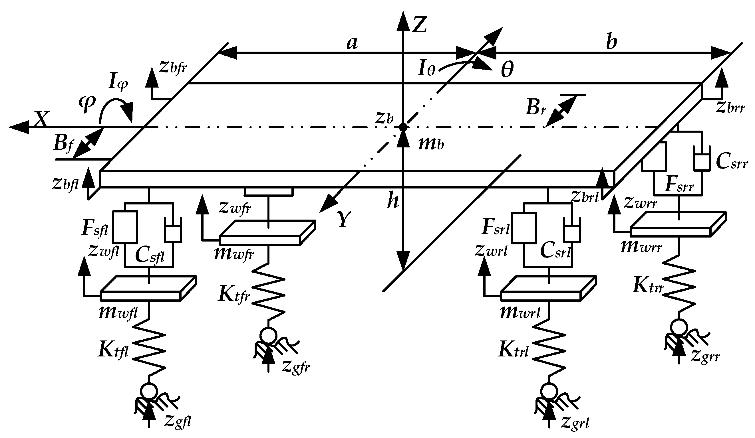
Figure 3.
Vehicle height adjustment system.
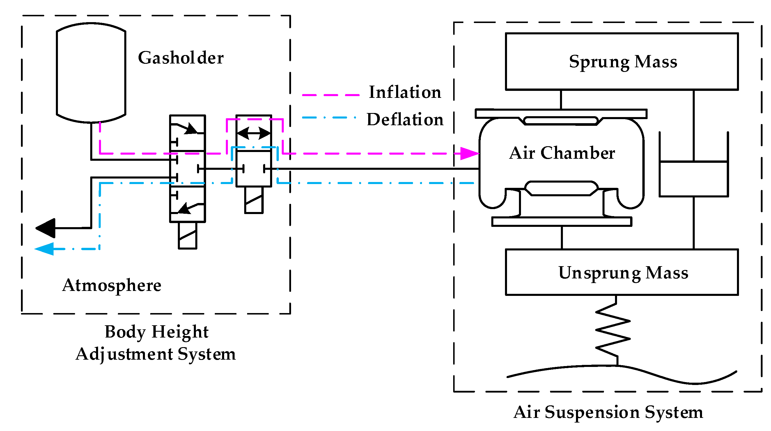
Figure 4.
Flow chart of control strategy: (a) Adjustment according to the dynamic deflection; (b) Adjustment according to static equilibrium position.
Figure 4.
Flow chart of control strategy: (a) Adjustment according to the dynamic deflection; (b) Adjustment according to static equilibrium position.

Figure 5.
Phenomena during the process of height adjustment.
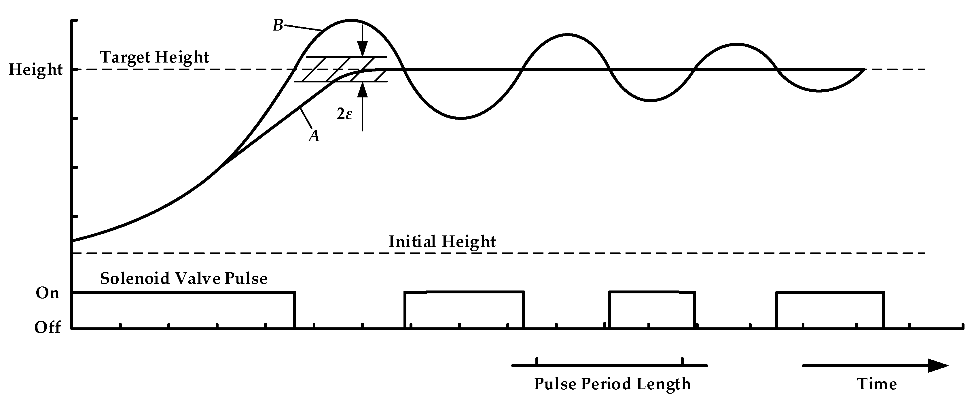
Figure 6.
Iteration of UKF.

Figure 7.
Membership function of input variables: (a) error; (b) change rate of error.

Figure 8.
System responses after solenoid valves open at 2 s: (a) intake valve opening; (b) exhaust valve opening.
Figure 8.
System responses after solenoid valves open at 2 s: (a) intake valve opening; (b) exhaust valve opening.

Figure 9.
System responses: (a) front left suspension; (b) rear left suspension.
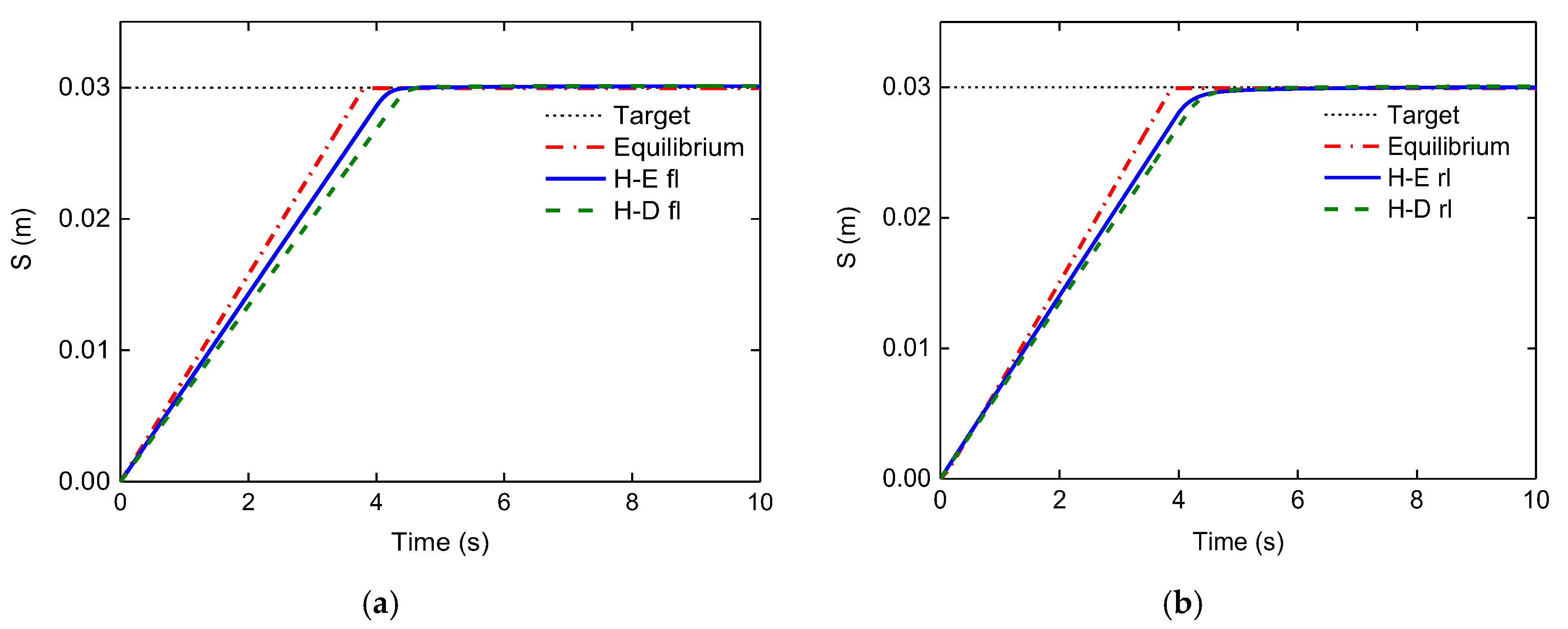
Figure 10.
System responses: (a) height change; (b) pitch angle change.

Figure 11.
System responses: (a) front left suspension; (b) rear left suspension.

Figure 12.
System responses: (a) height change; (b) pitch angle change.

Figure 13.
Excitation signal of a speed bump.

Figure 14.
System responses: (a) front left and front right suspensions; (b) rear left and rear right suspensions.
Figure 14.
System responses: (a) front left and front right suspensions; (b) rear left and rear right suspensions.
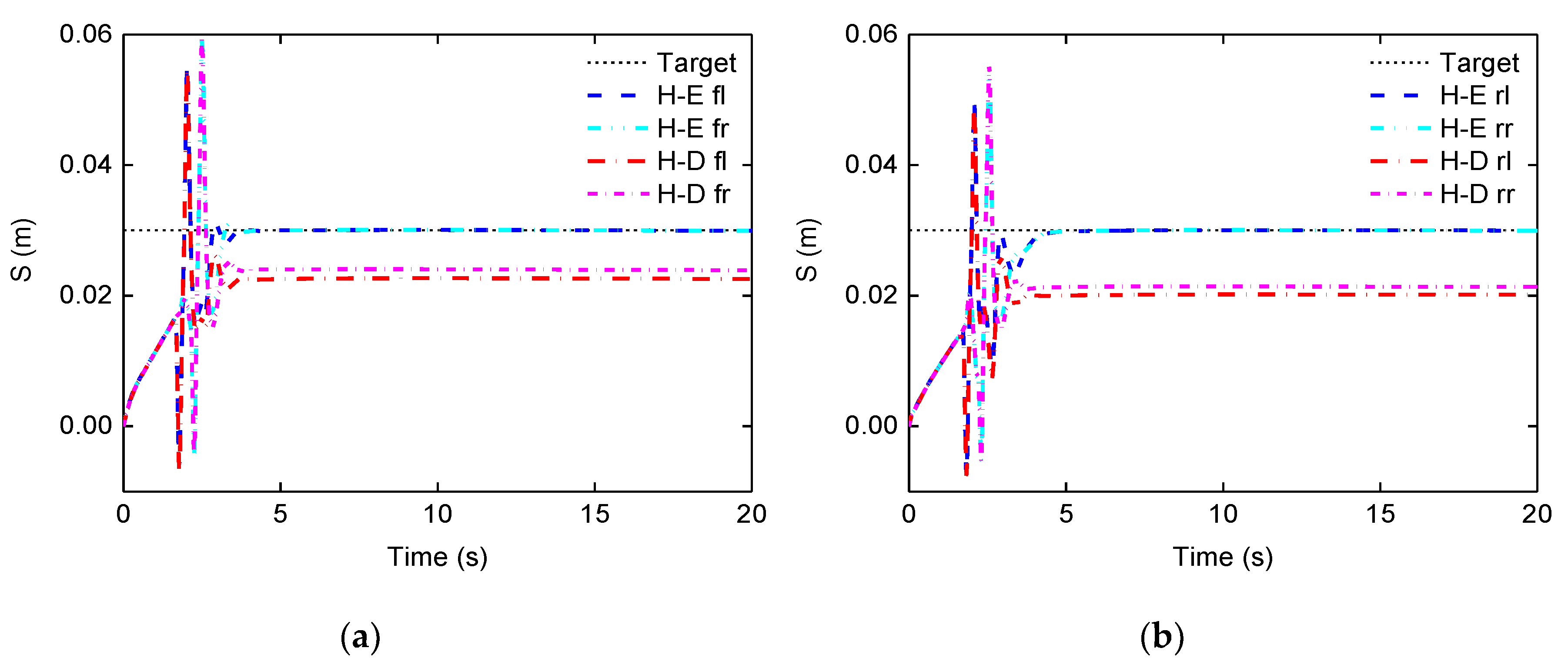
Figure 15.
System responses: (a) height change; (b) pitch angle change.
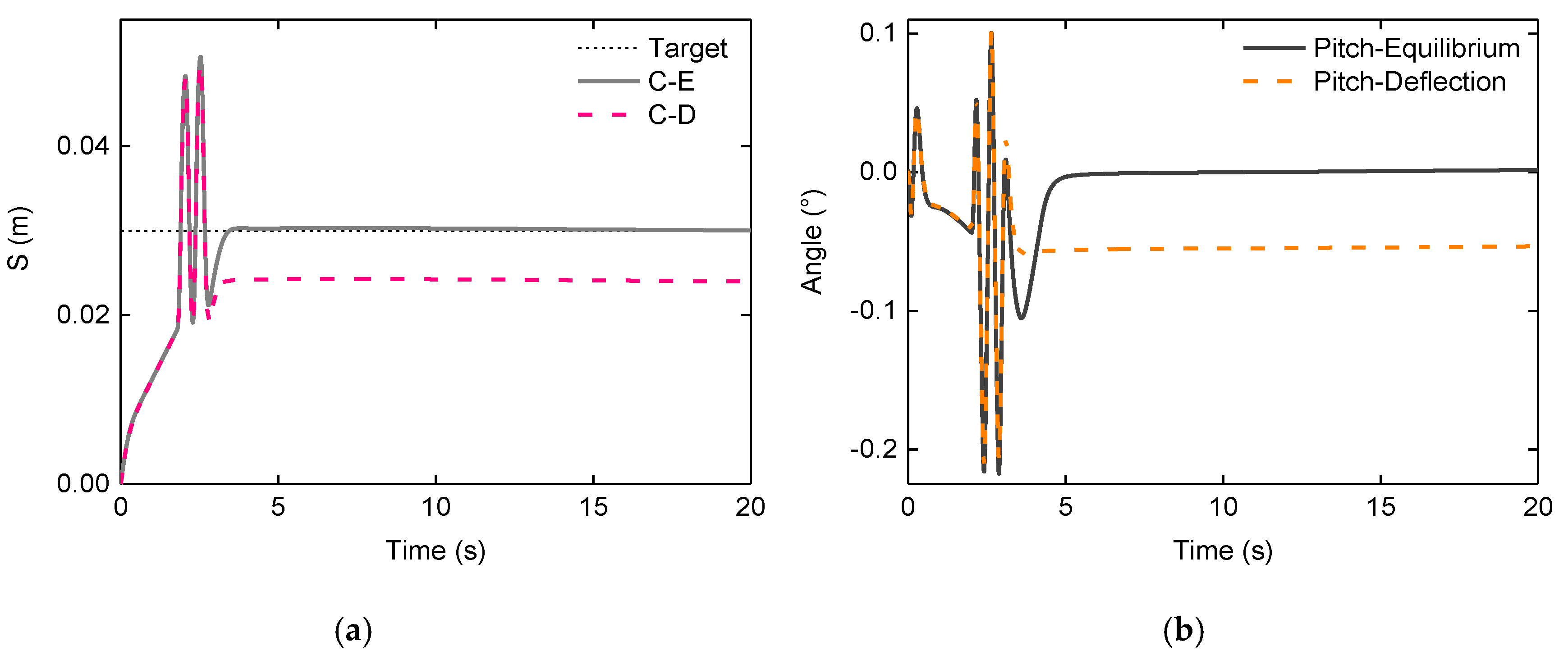
Figure 16.
System responses: (a) front left suspension; (b) rear left suspension.

Figure 17.
System responses: (a) height change; (b) changes of pitch angle and roll angle.
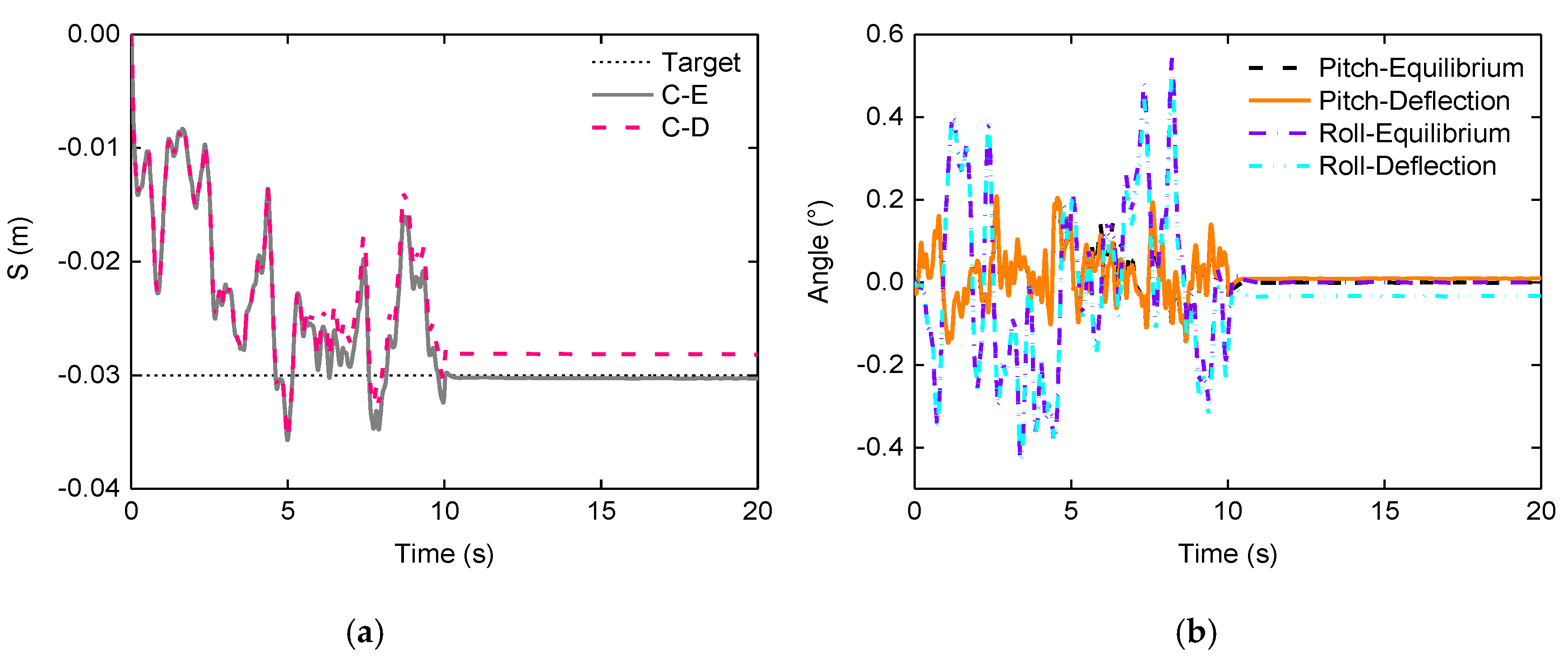
Figure 18.
Vehicle test.
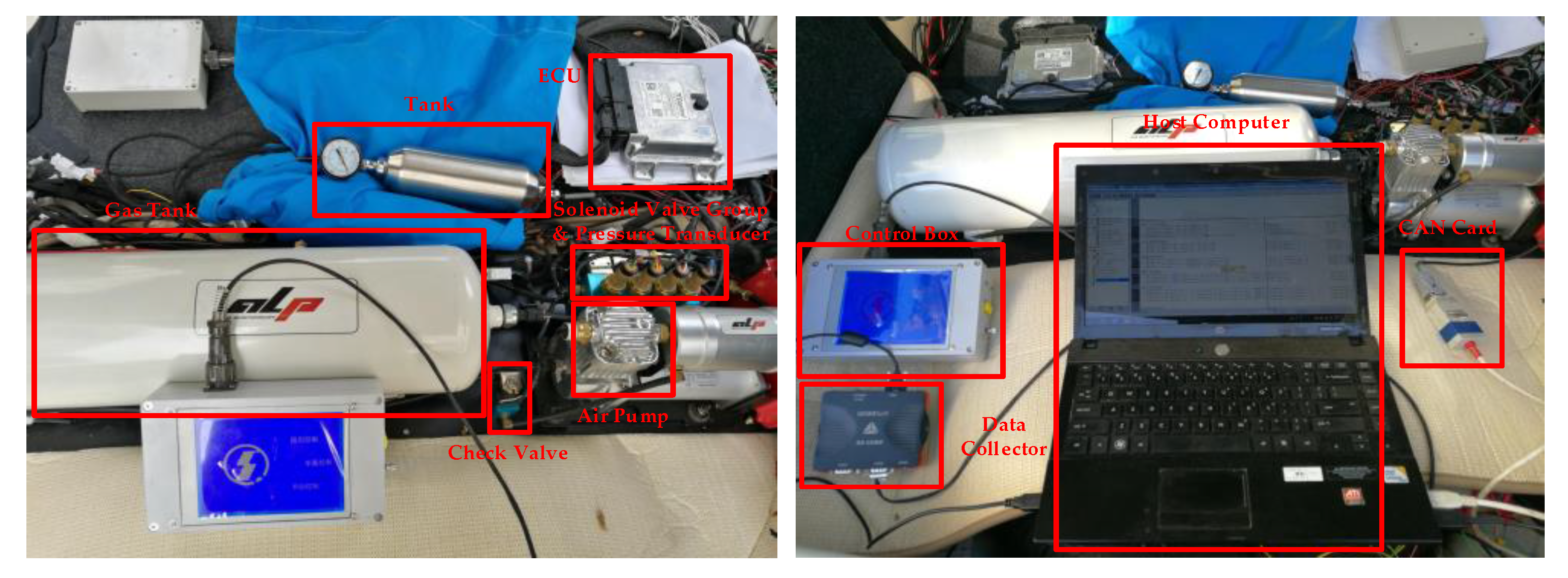
Figure 19.
Air suspension stiffness characteristics.
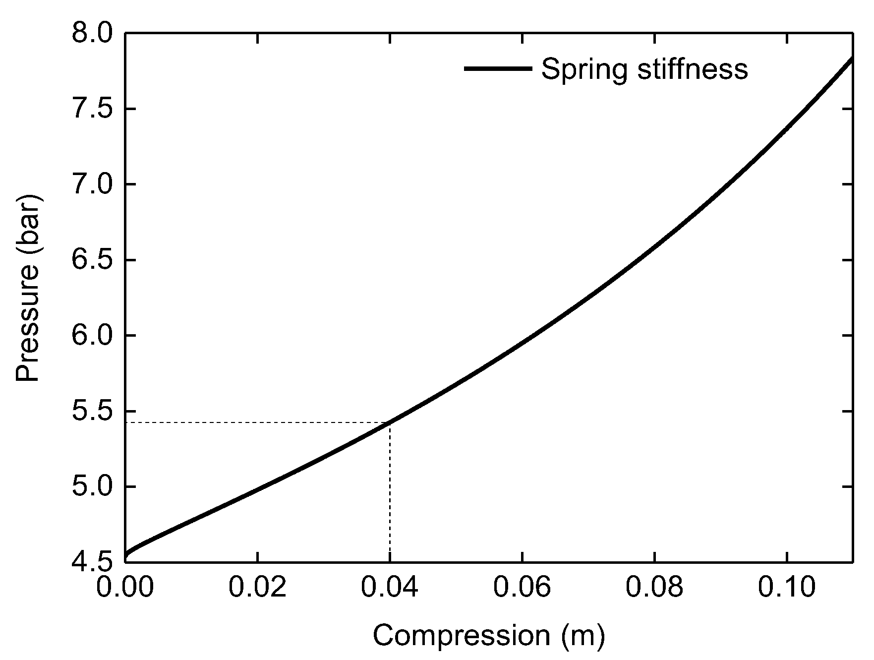
Figure 20.
Pressure changes: (a) inflating; (b) deflating.

Figure 21.
Vehicle centroid height changes: (a) suspensions inflating; (b) suspensions inflating.
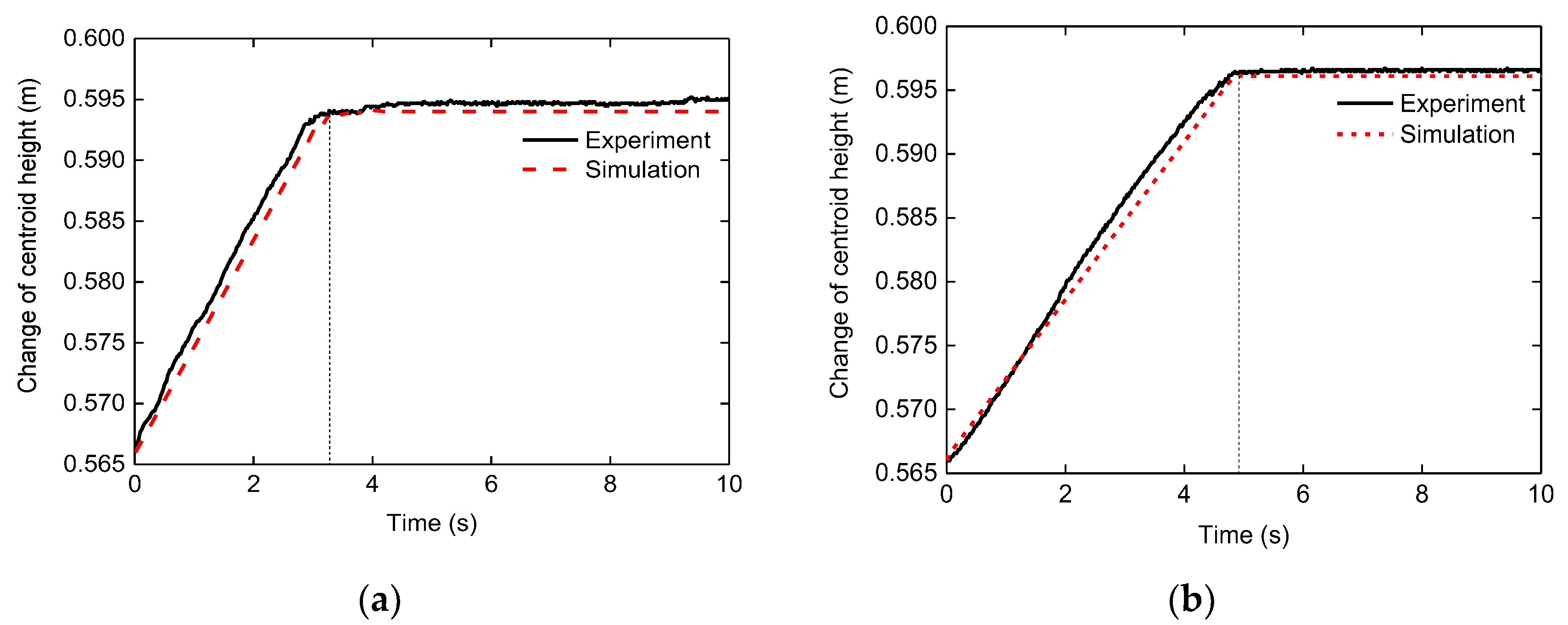
Figure 22.
Height changes: (a) suspension inflating; (b) suspension deflating.
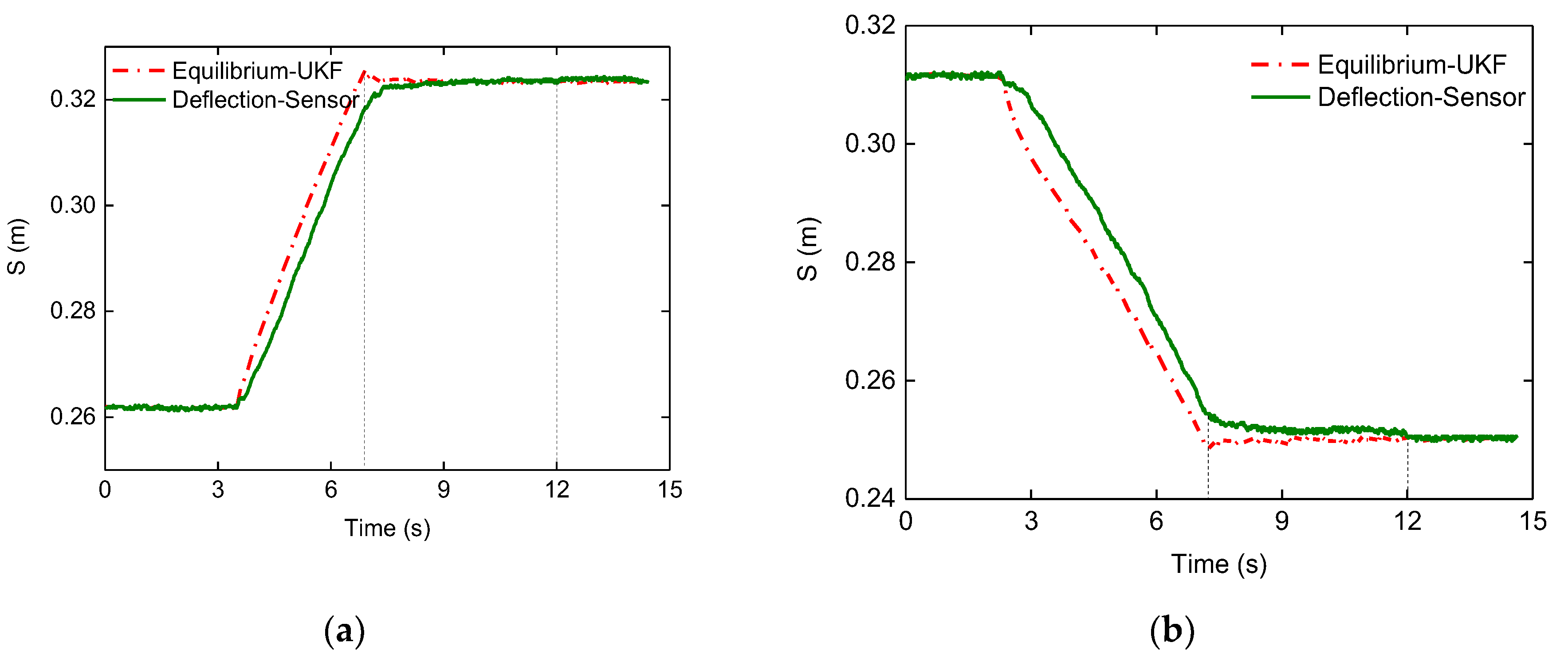
Figure 23.
Height changes: (a) height lifting; (b) height lowering.

Figure 24.
Error changes: (a) height lifting; (b) height lowering.
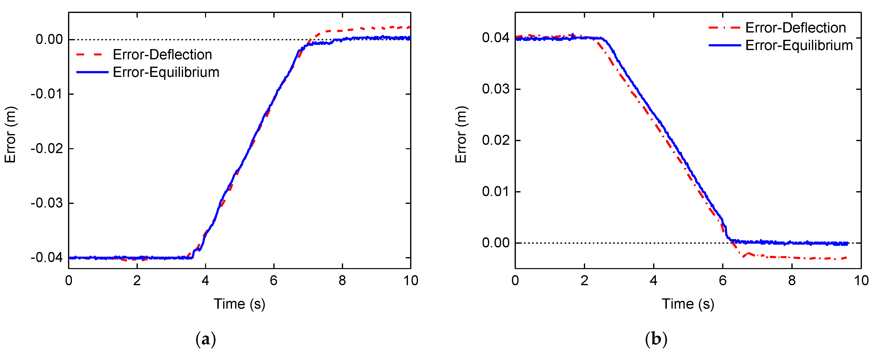
Figure 25.
Height changes: (a) height lifting; (b) height lowering.
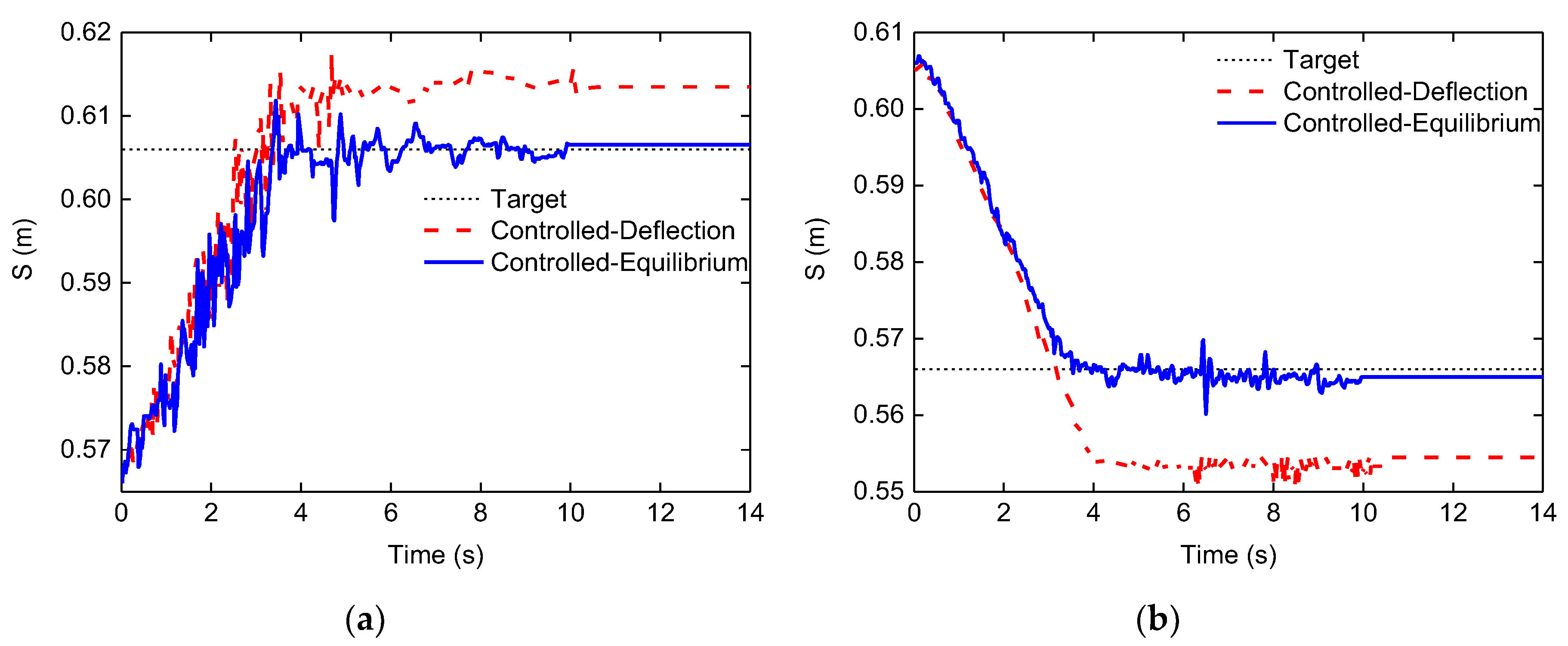
Figure 26.
Error changes: (a) height lifting; (b) height lowering.

Figure 27.
State of solenoid valve: (a) intake solenoid valve; (b) exhaust solenoid valve.


Table 1.
The linguistic rules table.
| DEE | XXS | XS | S | M | L | XL | XXL |
|---|---|---|---|---|---|---|---|
| NSS | NNS | NNS | NNS | NNS | NNS | NNS | NS |
| NS | NNS | NNS | NNS | NNS | NNS | NS | NS |
| N | NNS | NS | NS | S | M | B | PB |
| Z | S | S | M | B | PB | PB | PPB |
| P | S | M | B | B | PB | PPB | PPB |
| PB | M | B | B | PB | PPB | PPB | PPB |
| PPB | B | PB | PB | PPB | PPB | PPB | PPB |
Table 2.
Parameters of electric vehicle system.
| Parameters | Value | Parameters | Value |
|---|---|---|---|
| mb | 1000 kg | Cs | 5 kNs/m |
| mt | 42 kg | Kt | 232 kN/m |
| a | 1.05 m | A | 78.54 cm2 |
| b | 1.6 m | Ae | 3.14 mm2 |
| h | 0.566 m | L | −60 ~ 50 mm |
| Iθ | 2566.29 kg·m2 | R | 287 J/(kg K) |
| Iφ | 753.31 kg·m2 | D | 0.1 m |
| B | 1.5 m | g | 9.81 m/s2 |
© 2018 by the authors. Licensee MDPI, Basel, Switzerland. This article is an open access article distributed under the terms and conditions of the Creative Commons Attribution (CC BY) license (http://creativecommons.org/licenses/by/4.0/).
Share and Cite
MDPI and ACS Style
Gao, Z.; Chen, S.; Zhao, Y.; Nan, J. Height Adjustment of Vehicles Based on a Static Equilibrium Position State Observation Algorithm. Energies 2018, 11, 455. https://doi.org/10.3390/en11020455
AMA Style
Gao Z, Chen S, Zhao Y, Nan J. Height Adjustment of Vehicles Based on a Static Equilibrium Position State Observation Algorithm. Energies. 2018; 11(2):455. https://doi.org/10.3390/en11020455
Chicago/Turabian StyleGao, Zepeng, Sizhong Chen, Yuzhuang Zhao, and Jinrui Nan. 2018. "Height Adjustment of Vehicles Based on a Static Equilibrium Position State Observation Algorithm" Energies 11, no. 2: 455. https://doi.org/10.3390/en11020455
Note that from the first issue of 2016, this journal uses article numbers instead of page numbers. See further details here.