Prediction Model of Photovoltaic Module Temperature for Power Performance of Floating PVs


1
Konkuk University, 120 Neungdong-Ro, Gwanjin-Gu, Seoul 143-701, Korea
2
LSIS R&D Campus 116 beongil 40 Anyang, Gyeonggi 431-831, Korea
*
Author to whom correspondence should be addressed.
Energies 2018, 11(2), 447; https://doi.org/10.3390/en11020447
Submission received: 13 December 2017
/
Revised: 9 February 2018
/
Accepted: 11 February 2018
/
Published: 18 February 2018
(This article belongs to the Special Issue PV System Design and Performance)
Abstract
:Rapid reduction in the price of photovoltaic (solar PV) cells and modules has resulted in a rapid increase in solar system deployments to an annual expected capacity of 200 GW by 2020. Achieving high PV cell and module efficiency is necessary for many solar manufacturers to break even. In addition, new innovative installation methods are emerging to complement the drive to lower $/W PV system price. The floating PV (FPV) solar market space has emerged as a method for utilizing the cool ambient environment of the FPV system near the water surface based on successful FPV module (FPVM) reliability studies that showed degradation rates below 0.5% p.a. with new encapsulation material. PV module temperature analysis is another critical area, governing the efficiency performance of solar cells and module. In this paper, data collected over five-minute intervals from a PV system over a year is analyzed. We use MATLAB to derived equation coefficients of predictable environmental variables to derive FPVM’s first module temperature operation models. When comparing the theoretical prediction to real field PV module operation temperature, the corresponding model errors range between 2% and 4% depending on number of equation coefficients incorporated. This study is useful in validation results of other studies that show FPV systems producing 10% more energy than other land based systems.
1. Introduction
A report published by International Renewable Energy Agency (IRENA) in 2016 [1] shows that the global cumulative capacity of installed solar systems was 222 GW, with China, Germany, Japan, and USA installing 43, 40, 33, and 22 GW, respectively. In many markets, we see the growing conflict between the need to convert arable land or forests to create PV installation sites installation vis-à-vis the need to protect the environment. A floating photovoltaic (PV) system installation on dams or water reservoirs is one such method that offers an installation site option with minimal interference with the environment. Additionally, it utilizes the cooling effect of water on its surface to improve the efficiency of the PV module and ultimately the performance of the PV system [2].
Extensive studies on the efficiency, power, and temperature of the conventional PV system module have been carried out by Evans [3], Duffie and Beckman [4], and many others [5]. Considering the importance of device temperature in PVM efficiency analysis, this paper proposes a model that correlates the temperature of a FPV module to the ambient temperature, solar radiation, and wind speed. A second model incorporates the influence of water temperature of the FPV installation. Well known PV module temperature models are compared under constant irradiation and constant ambient conditions as presented herein. The characteristic analysis of the FPVM temperature models shows resemblance to models proposed by Lasnier and Ang 1990 [6] and Duffie and Beckmans 2006. Duffie and Beckmans’ predictions are thus preferred for size optimization, simulation and design of solar photovoltaics. Koehl [7], Kurtz [8], and Skoplaski [9] that include wind speed in temperature predictions are also included in analysis. A simple comparison of the temperature profiles of FPVMs with the conventional land- or rooftop-based modules shows that the mean value of the yearly PV module temperature of an FPV system is 21 °C, which is 4 °C below that of land or rooftop installed PV modules [10].
The aforementioned research is important in analyzing the correlation between efficiency and temperature. Solar cells only convert a small amount of absorbed solar radiation into electrical energy with the remaining energy being dissipated as heat in the bulk region of the cell [11]. A rise in the operation temperature of a solar cell and module reduces the band gap, thus slightly increasing the short circuit current of a solar cell for a given irradiance, but largely decreasing the open circuit voltage, resulting in a lower fill factor and power output. The net effect results in a linear relation for the electrical efficiency () of a PV module as
where and are the electrical efficiency and temperature coefficient of the PV module, respectively. and are the PV module operational temperature and reference temperature, respectively.
2. Floating PV System Introduction and Performance
2.1. Site Information of Floating PV System
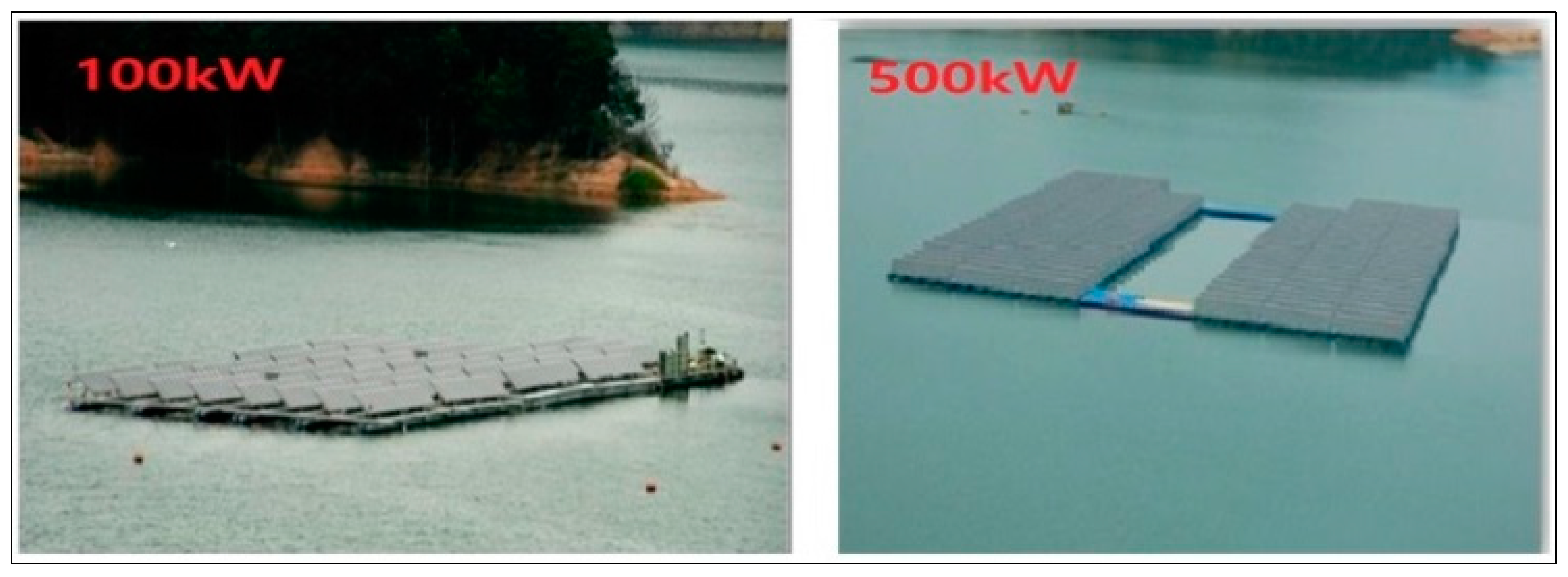
Figure 1 shows the aerial views of Korea’s first 100 kW and 500 kW Hapcheon Dam FPV power stations located at southern part of the country. Based on the previous research on module reliability [2], a special anti-damp proof FPVM with a unique encapsulation was certified and installed. A unique mooring system is anchored the floating system on the dam floor, aligning the FPV system to the correct azimuth. To monitor environment conditions, a portion of the floating platform is fitted with a small weather station equipped with sensors, as outlined in Table 1, and based on IEC (International Electrotechnical Commission) standard 61724-1 [12]. A low-loss cable transmitted DC power from the FPV system to dry land where an electric room housing a PV inverter and monitoring computers were installed.
2.2. Power Outputs of Floating PV Versus Rooftop-Based System
In Table 2, we outline system specification of two FPV and a land based systems study.
Table 3 shows yearly energy results of the three PV systems. We compare the performance of the three systems after normalizing energy output with system kWp capacity (kWh/KWp). The unit (h/d) is an expression of how many hours a PV system operates at its peak power. As shown in Table 3, the y-axis (left) illustrates this daily monthly average energy output. For example in April 2013, average monthly output from the three PV Systems was 443, 2078, and 3976 kWh for the 100, 500, and 1000 kW PV systems, respectively. Multiplying respective monthly average but days in month, and summing monthly outputs gives 130.3, 693.2, and 1197.5 MWh respective total yearly output.
For the 100 kW FPV station, October and December are the best and worst performing months at 445 kWh and 264 kWh respectively, compared to the station’s yearly average of 357 kWh. Similarly for the 500 kW FPV station, March and December are the best and worst performing months at 2316 kWh and 1512 kWh respectively, compared to the station’s yearly average of 1859 kWh. Finally for the 1000 kW rooftop PV station, May and December are the best and worst performing months at 3998 Wh and 2612 kWh respectively, compared to the station’s yearly average of 3281 kWh. Whereas the rooftop produces more power quantitatively, the FPV systems are more efficient in qualitative power delivery. Output energy (kWh) normalization to name plate peak power (kWp) results in hours per day (h/day) unites. Table 3 shows an average of all monthly values gives yearly normalized output of 3.58, 3.80, and 3.28 h/day, respectively, as shown in Table 3. Analysis of the latter values proves the two FPV systems are outperforming the rooftop systems by 9% and 16%, warranting investigation into temperature performance.
3. Methodology of Floating PV Temperature Model
In this section, we formulate a multiple linear equation for the dependent PVM variable (y; FPV module operation temperature) using four independent linear variables , , and representing solar irradiance (), ambient temperature (), wind speed (), and water temperature (), respectively.
The equation is linear for unknown parameters , and is of the form given in Equation (2)
where is the predicted value of module temperature and assumes ith independent error following a normal distribution with independent mean and variance squared. The matrix can be expressed as
where and .
The multiple linear regression form is expressed in Equation (3) with Y, β, ϵ, and X representing y observations, vector of parameters, error, and matrix vectors, respectively. The field data of PV system data is given in the forms of for , respectively.
We use the standard least-squares minimization to determine the aforementioned model parameters by minimizing the sum of squares of residuals () as shown in a matrix form in Equation (4)
where , and .
Substituting the former into Equation (4) leads to the definition of in terms of the unknown parameters in Equation (5).
Equation is expanded using . Integrating with respect to results in normal equations, which have to be solved for unknown equations in Equation (6). For easy computation, an alternative matrix equation is presented for solving the coefficients.
where is the inverse matrix of predictor variables listed on Table 4.
4. FPV Temperature Model Results and Comparisons
4.1. Model Results
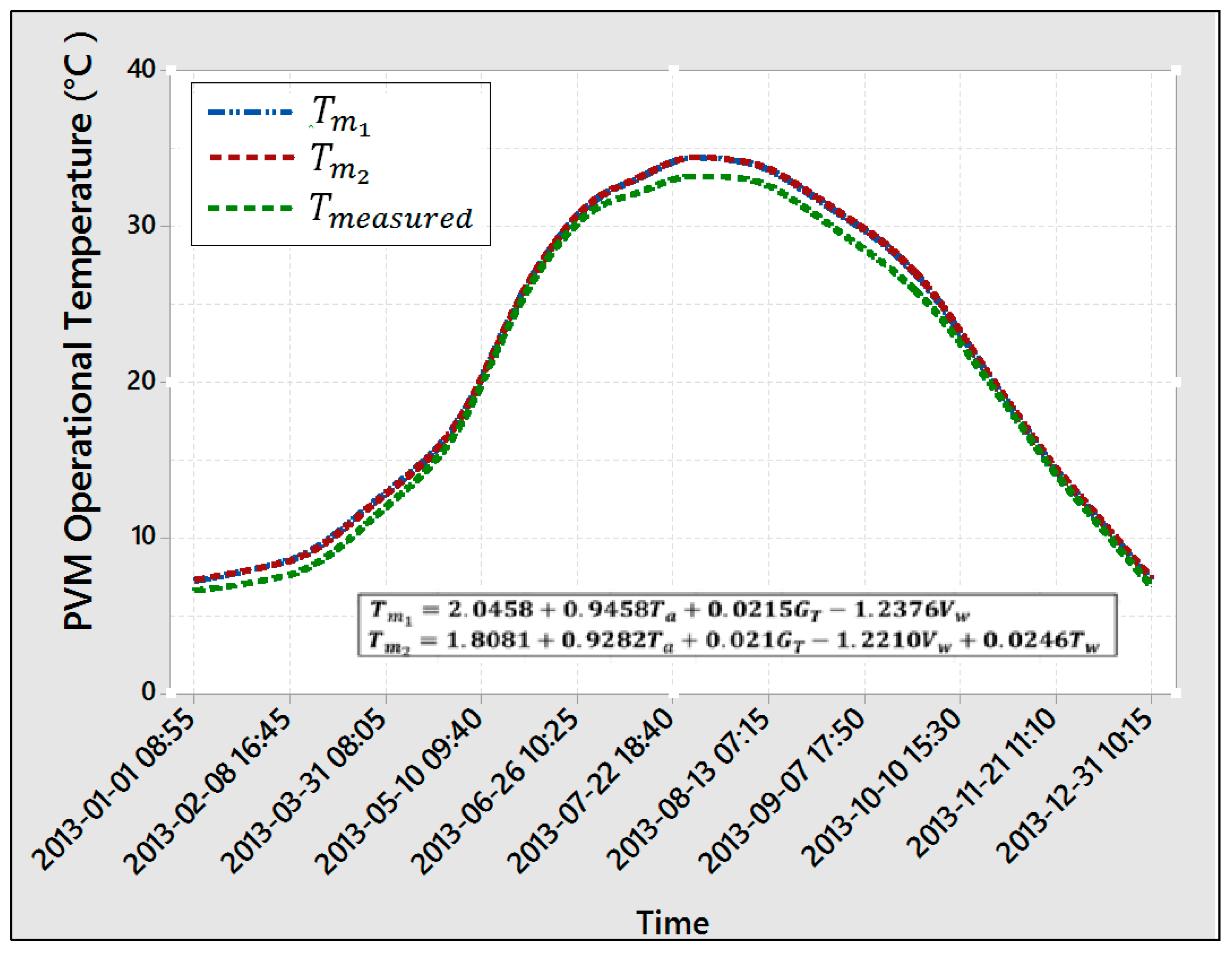
With data collected from the floating PV site, we formulate the X matrix containing FPVM data points, as is plotted in Figure 3, and corresponds to five minutes of site data. The Y matrix corresponds to the measured module temperature. The coefficients of models 1 and models 2 in Equation (4) for the FPVM suggested in this paper are expressed as
and explains the operation temperature behavior of the FPV module with seasonal variables ,, , and .
Based on the two predictions of the temperature of an FPVM proposed herein, we propose two corresponding modifications to Equation (1) based on the input parameters of as
where ,, and represent average values of corresponding model PV module efficiency, ambient temperature, solar irradiation, and wind speed respectively. Equation (9) includes an additional variable, i.e., water temperature ().
Figure 3 is a time series plot of predicted and measured module temperatures in 2013. From the graph, predicted PVM temperatures are almost always higher than measured except during third quarter where , . Coincidentally, wind speeds () are also low during same period, implying the dominance of in the two models Equations (8) and (9).
Equation (12) introduces the average error, as the difference in area of the curves of measured versus modeled temperatures in Figure 3 of FPV models, by showing the average difference between predicted and measured values. ranges between 2.06% and 4.40%, for respective FPV models.
In Equation (12), is total data points. Inclusion of in Equation (11) increases by 2% to 4%.
4.2. Comparison with Land-Based PV System
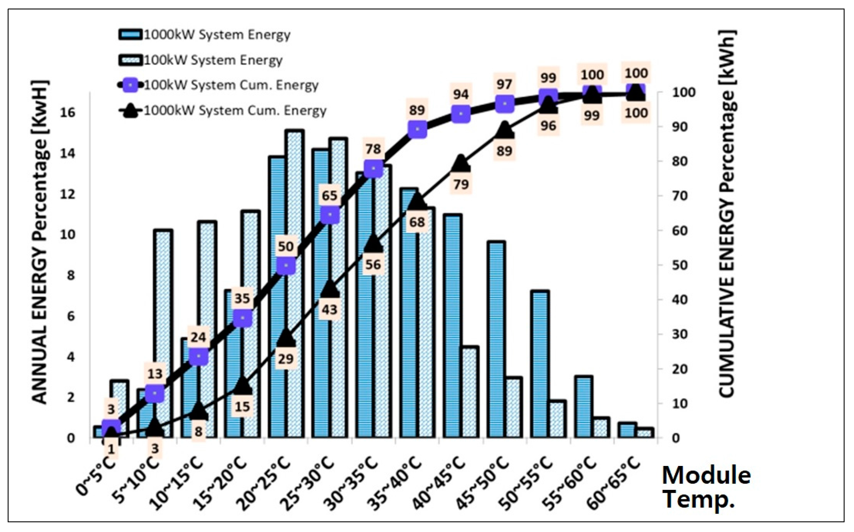
In Figure 4, we compare the floating PV and rooftop system yearly energy profile based on operation module temperature. As can be seen, the FPV system produces a larger portion of energy at lower temperatures [13] compared to the rooftop system.
Cumulative PV energy produced throughout the year, is plotted against corresponding module temperature. As indicated, 89% of annual energy produced by the FPV system, and 68% of the rooftop system’s energy is produced when module temperatures of both systems are below 40 °C. Energy produced beyond the 25 °C is subject to power loss due to loss of open circuit () and fill factor (F.F.).
4.3. Comparison with Selected Temperature Models
A select group of PV temperature models [5] is presented in Table 5 for comparison. The models incorporate a reference, stating for example air temperature (), and the corresponding values of relevant variables (, , etc.). Owing to the complexities involved, some authors presented explicit correlation in addition to implicit relations requiring iterations.
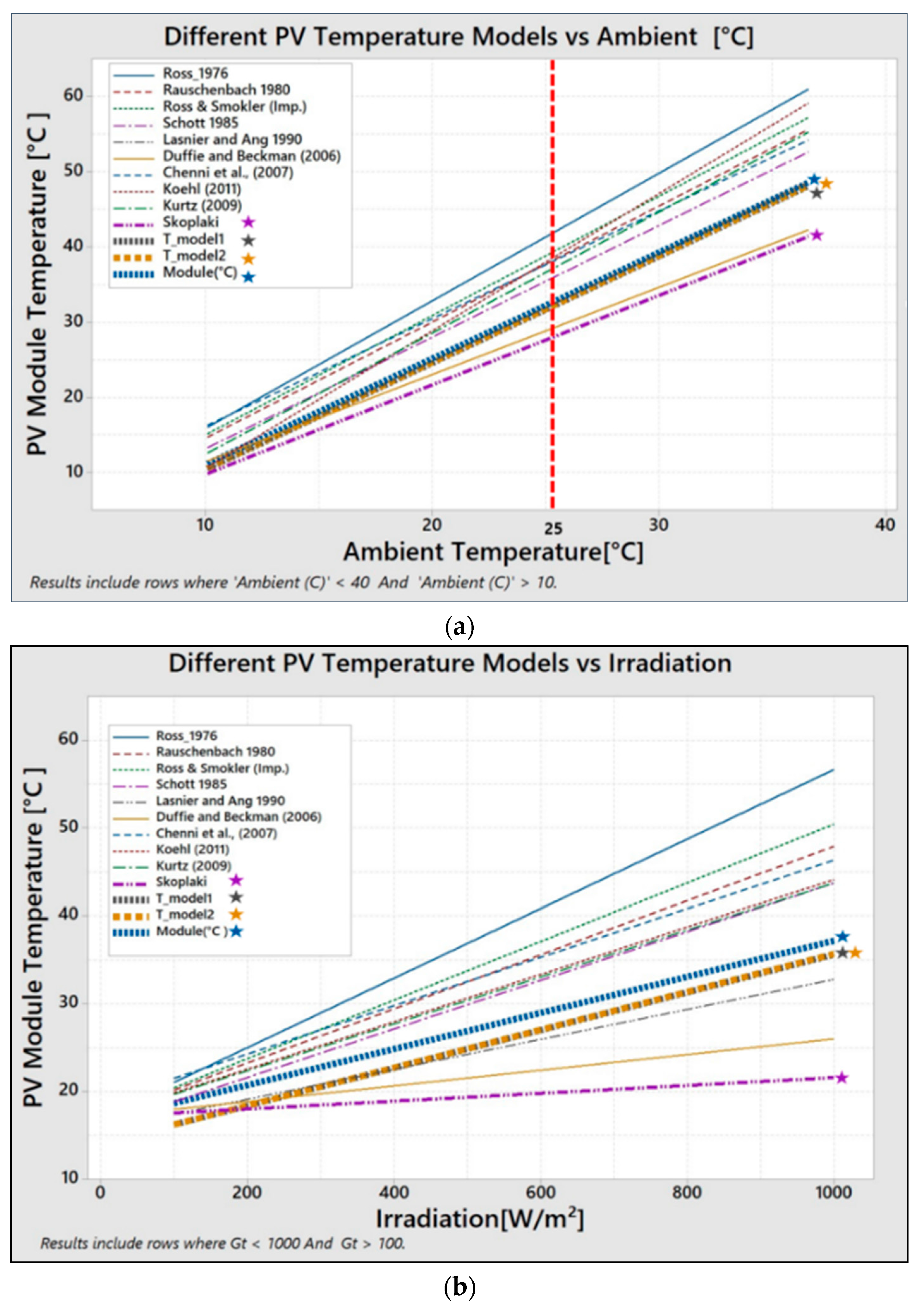
In Figure 5 below, temperature models listed above are plotted against both ambient () temperature and solar radiation ().
As can be seen, all models vary linearly with both and with varying specific gradients. The analytical implication is different model interpret heat dissipation by the PV module differently when exposed to the elements. For example, Ross [14] and Rauschenbach [15] model display the highest PV operation temperatures when exposed to at constant . Koehl, Kurtz, and Skoplaki’s research incorporates wind () data in temperature prediction.
In Figure 5a, Duffie & Beckman [4] and Skoplaki [9] recorded low temperatures with increasing , suggesting adequate heat dissipation by the modules due to incorporation of wind data. To the contrary, Ross and Rauschenbach show high temperatures near 60 °C suggesting the PVM retains heat.
Model 1 () and Model 2 () plots vary slightly with real PV module data, and operate at much lower temperatures when compared to all other models. Lower operation temperatures suggests heat dissipation to FPV ambient environment
In Figure 5b, Skoplaki has lowest operation temperature with increasing , while Ross has highest temperature values because of PVM heat retention. Skoplaki model reacts very slowly to rising due to quick heat dissipation by the factor. A slight deviation from real temperature by Model 1 () and Model 2 () is noted with increasing .
Based on the two graphs in Figure 5, we conclude that our two FPV models operating temperatures are significantly lower than conventional PV module ranges.
4.4. Comparison of Models with Minitab Model
MINITAB [18] is an advanced statistics program has well-defined algorithms that describe the change of any dependent variablewith the interaction between the respective independent variables. Minitab generates an equation that shows the interaction between the dependent variable (module temperature) and independent variables. Equation (13) derived by MINITAB is highly accurate (0.1%) but incurs the risk of equation complexity due to over-fitting.
for , representing .
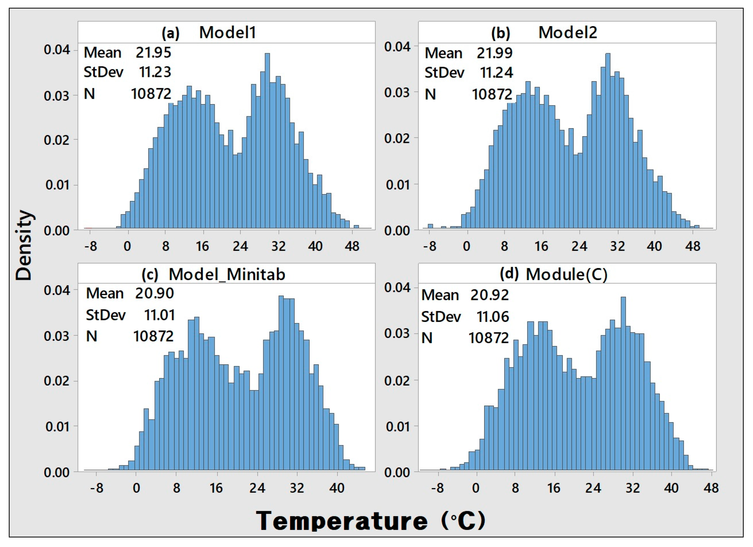
In Figure 6, four histograms compare the normal distribution of real FPV module temperature data (lower right) to Model 1, Model 2, MINITAB’s prediction.
The sub figures x-axis is operational temperature from −10 °C to over 50 °C. The y-axis plots the density of respective temperature range throughout the year. All model distributions show a bimodal shape, with two peaks temperatures at 10 °C and 30 °C. Analysis with fewer data points shows a normal distribution curve.
5. FPV Module Efficiency and Power Prediction
Operating a PV system on the water surface has the added benefit of increasing conversion efficiency due to the cooling effect on water’s surface.
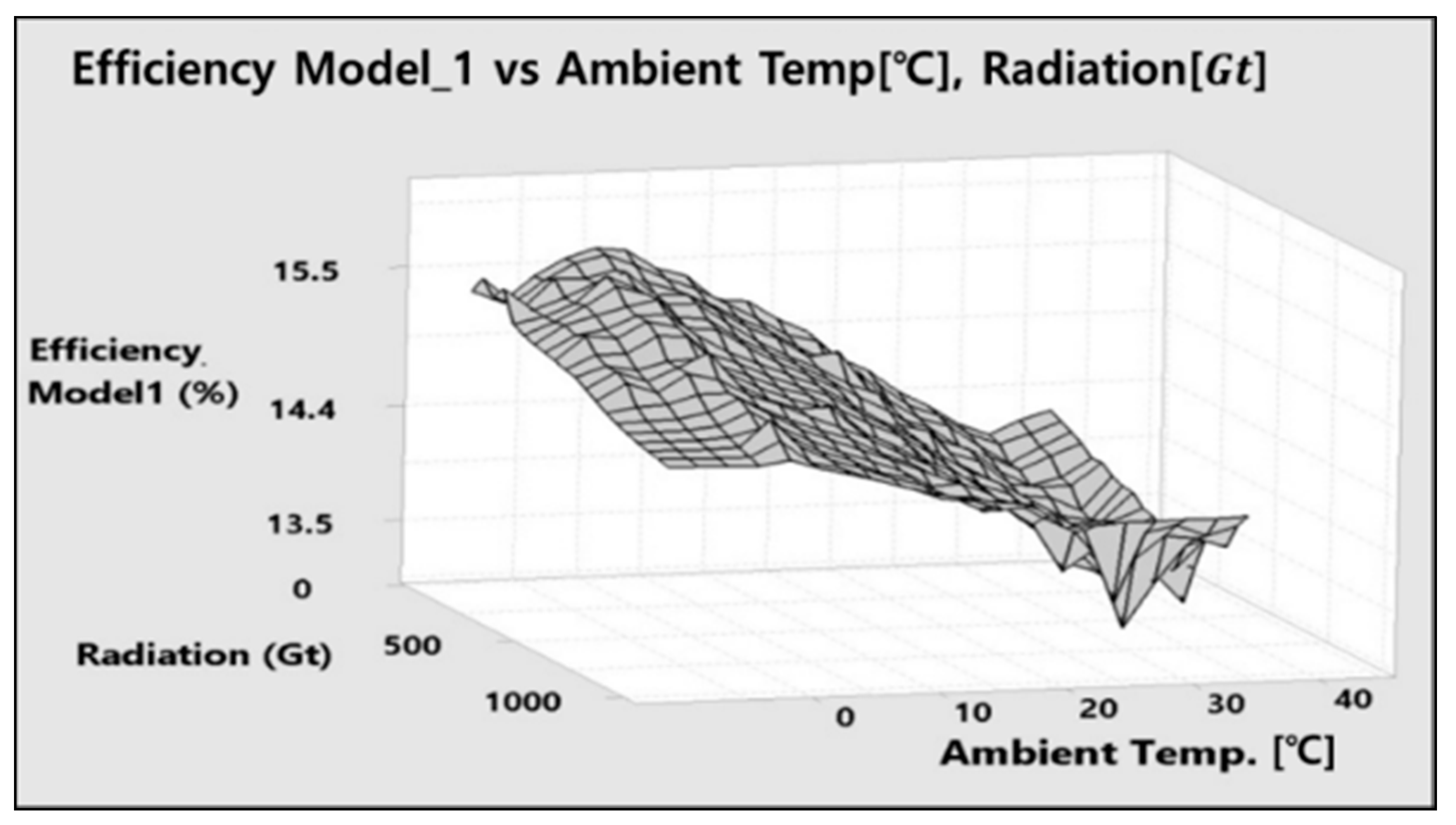
Figure 7 is a 3D plot of FPV module efficiency//. In the plot, a decrease in ambient temperature () has a positive effect of increasing efficiency between 1–2% points. The plot shows the importance in defining PVM operation temperature and, ultimately, conversion efficiency. Radiation () plays a secondary role given the minimal impact on efficiency. It can be observed that, at higher radiation levels, varies more frequently, and this impacts power stability.
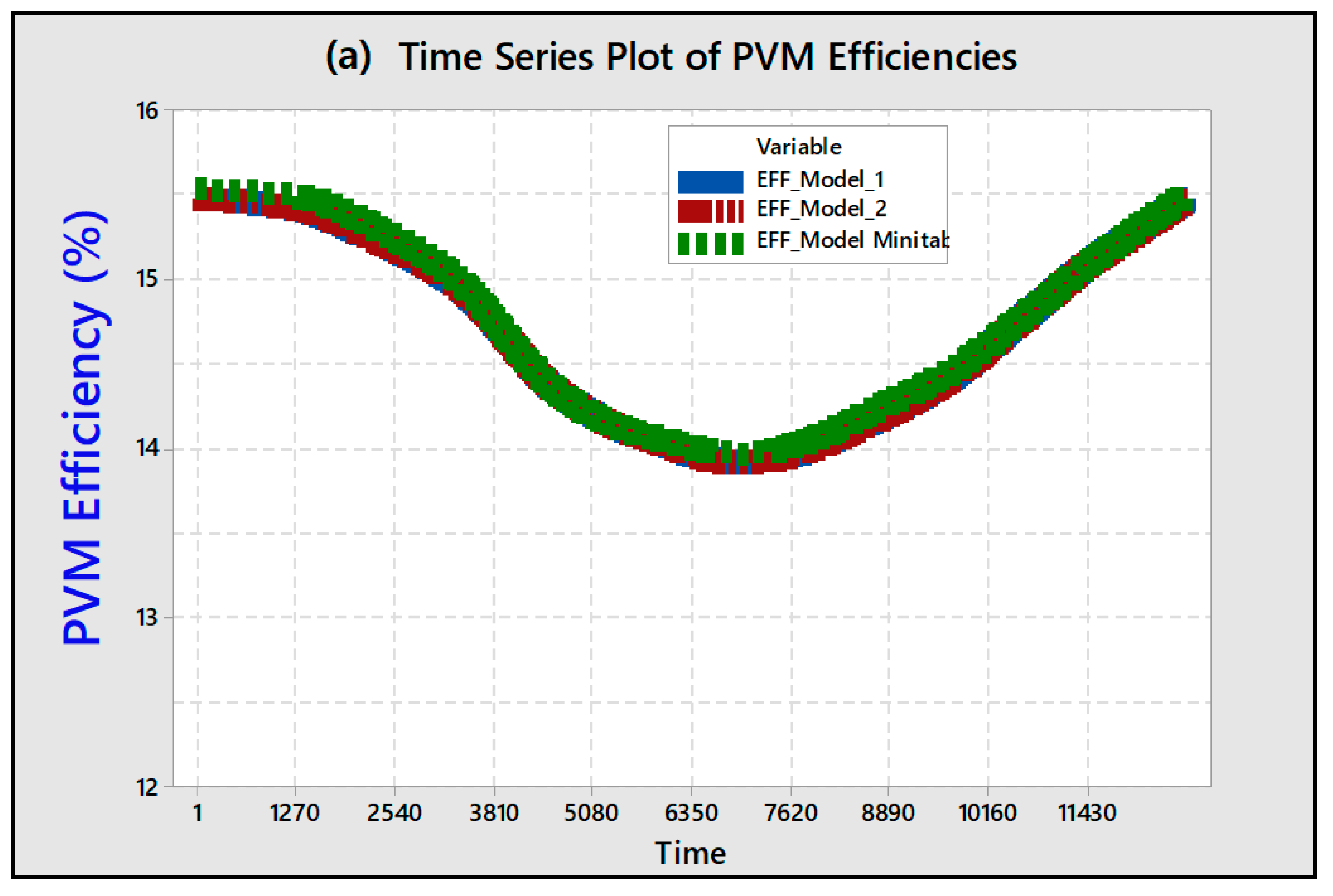
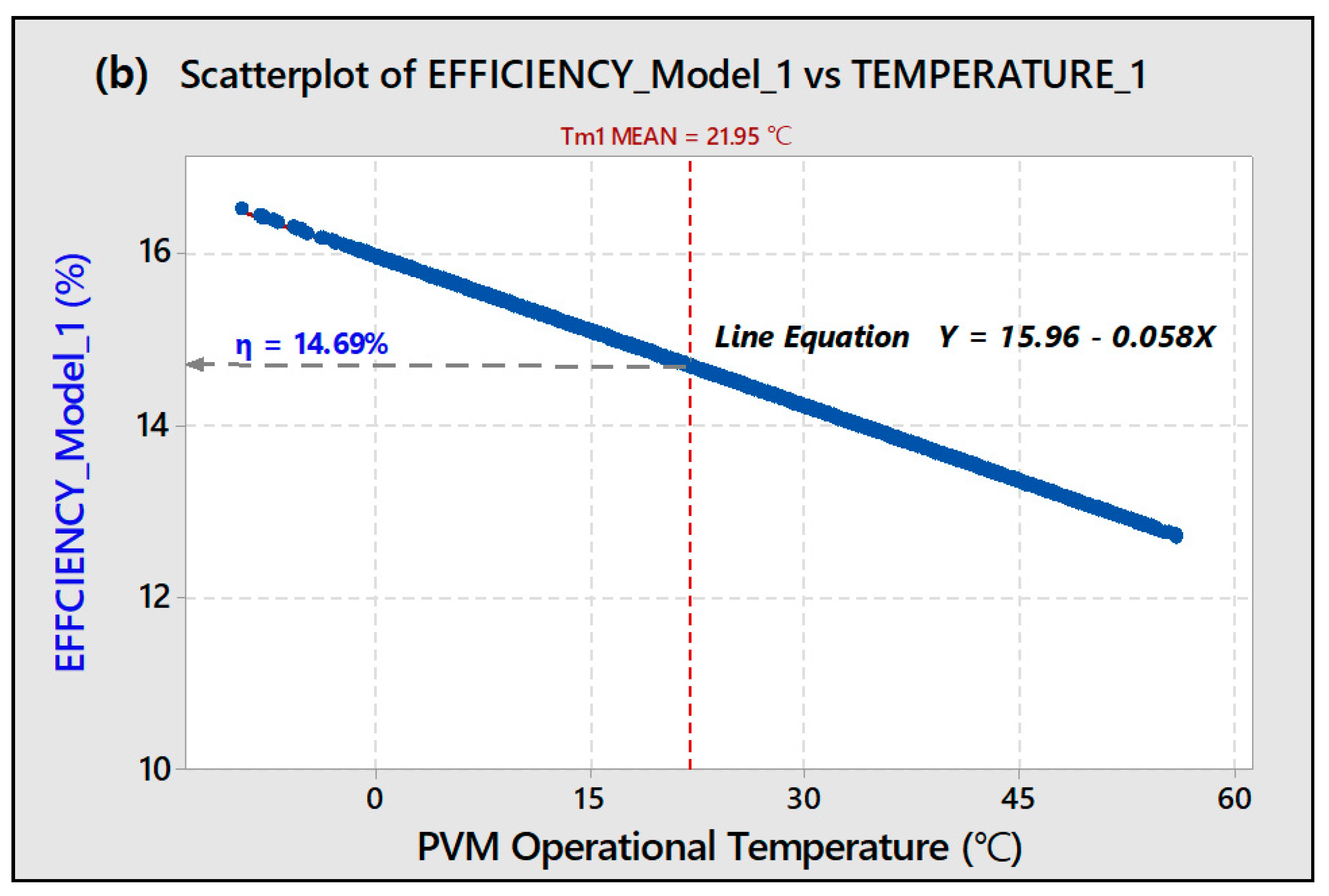
In summary, as observed from the FPV data, low ambient conditions are ideal for higher system efficiency and power performance as shown by seasonal variation in efficiency in Figure 8. In June through August when ambient temperature are high, PVM efficiency drops between 1–2% points. For a land based system, a more severe dip is expected. During fall and winter when temperatures drop, we notice a step rise in efficiencies to the mid-15% level. Based on graphical description on Figure 8, for FPV module temperature models 1, we predict that a 1 °C increase in results in a 0.058% decrease in , model 1 PVM efficiency, as shown for in Equation (14).
PV module operational temperature has an important role in the energy conversion process [19]. From Figure 8, the electrical efficiency of the PV module varies linearly with temperature as shown. From the graph above for Model 1, Latifa [20] has done important work (2014) comparing crystalline (c-Si) and amorphous silicon (a-Si) coefficients per °C. This work shows coefficient values for a-Si closely identical to FPV.
6. Conclusions
Two prediction models of the FPV module operation temperature are suggested for the analysis of performance of the FPV module and system. Model 1 includes the effects the independent variables, i.e., ambient temperature (Ta), solar irradiance (Gt), and wind speeds (Vw). When compared to the measured FPV module temperature over entire year, the error of model 1 is 2%. Model 2 includes the three aforementioned independent variables in addition to water temperature (Tw). Although the error of Model 2 increases slightly to 4%, the results are within the reasonable range of error. Fitting of the experimental data is reproduced with a minor error.
Through this research, a correlation between the temperature of the floating PV operating environment and system efficiency is derived. Beyond solar irradiation of 100 W/m², the floating system records an ideal efficiency averaging more than 14.69% based on a yearly mean PVM temperature of 21.95 °C. It was also observed that approximately two-thirds of the annual yield produced by the FPV system occurs when the module operational temperature was below 40 °C.
Acknowledgments
This work was supported by the New and Renewable Energy Technology Program of the Korea Institute of Energy Technology Evaluation and Planning (KETEP) and granted financial resources from the Ministry of Trade, Industry and Energy, Republic of Korea (NO. 20153010012060). This paper was also written as part of Konkuk University’s research support program for its faculty on sabbatical leave in 2017.
Author Contributions
Waithiru Charles Lawrence Kamuyu developed his own primary model for the power with insolation environments, especially focusing on the photovoltaic module temperature. Jong Rok Lim added experimental data analysis with different seasons in two different areas. Chang Sub Won and Hyung Keun Ahn integrated the power tracing from the respect of environmental conditions to provide reliable temperature dependent tracking data for floating photovoltaic power station which is one of hottest systems these days for the micro-grid and land saving power network.
Conflicts of Interest
The authors declare no conflict of interest.
References
- International Renewable Energy Agency (IRENA). Solar PV in Africa: Costs and Markets; IRENA: Abu Dhabi, UAE, 2016; Chapter 3; p. 29. [Google Scholar]
- Won, C.; Waithiru, L.; Kim, D.; Kang, B.; Kim, K.; Lee, G. Floating PV Power System Evaluation Over Five Years (2011–2016 (EU PVSEC 2016)). In Proceedings of the 32nd European Photovoltaic Solar Energy Conference and Exhibition, Munich, Germany, 20–24 June 2016. [Google Scholar]
- Evans, D.L. Simplified method for predicting photovoltaic array output. Sol. Energy 1981, 27, 555–560. [Google Scholar] [CrossRef]
- Duffie, J.A.; Beckman, W.A. Solar Energy of Processes, 3rd ed.; Wiley: Hoboken, NJ, USA, 2006; p. 3. [Google Scholar]
- Jakhrani, A.Q. Comparison of Solar Photovoltaic Module Temperature Models. World Appl. Sci. J. Spec. Issue Food Environ. 2011, 14, 1–8. [Google Scholar]
- Lasnier, F.; Ang, T.G. Photovoltaic Engineering Handbook; Adam Hilger: New York, NY, USA, 1990; p. 80. [Google Scholar]
- Koehl, M.; Heck, M.; Wiesmeier, S.; Wirth, J. Modeling of the nominal operating cell temperature based on outdoor weathering. Sol. Energy Mater. Sol. C 2011, 95, 1638–1646. [Google Scholar] [CrossRef]
- Kurtz, S.; Whitfield, K.; Miller, D.; Joyce, J.; Wohlgemuth, J.; Kempe, M.; Dhere, N.; Bosco, N.; Zgonena, T. Evaluation of high-temperature exposure of rack mounted photovoltaic modules. In Proceedings of the 34th IEEE Photovoltaic Specialists Conference (PVSC), Philadelphia, PA, USA, 7–12 June 2009; pp. 2399–2404. [Google Scholar]
- Skoplaki, E.; Palyvos, J.A. On the temperature dependence of photovoltaic module electrical performance: A review of efficiency/power correlations. Sol. Energy 2009, 83, 614–624. [Google Scholar] [CrossRef]
- Young, K.C.; Nam, H.L.; Kern, J.K. Empirical Research on the efficiency of Floating PV systems compare with Overland Systems. In Proceedings of the 3rd International Conference on Circuits, Control, Communication, Electricity, Electronics, Energy, System, Signal and Simulation (CES-CUBE 2013), Tamuning, GU, USA, 18–20 July 2013; Volume 25, pp. 284–289. [Google Scholar]
- Green, M.A.; Blakers, A.W.; Shi, J.; Keller, E.M.; Wenham, S.R. High-Efficiency silicon solar cells. IEEE Trans. Electron Devices 1984, 31, 679–683. [Google Scholar] [CrossRef]
- IEC Standard 61724-1:2017, Photovoltaic System Performance—Part 1: Monitoring. Available online: https://webstore.iec.ch/publication/33622 (accessed on 1 July 2017).
- Malik, A.Q.; Ming, L.C.; Sheng, T.K.; Blundell, M. Influence of Temperature on the Performance of Photovoltaic. ASEAN J. Sci. Technol. Dev. 2010, 26, 61–72. [Google Scholar] [CrossRef]
- Ross, R.G. Interface design considerations for terrestrial solar cells modules. In Proceedings of the 12th IEEE Photovoltaic Specialist’s Conference, Baton Rouge, LA, USA, 7–10 January 1976; pp. 801–806. [Google Scholar]
- Rauschenbach, H.S. Solar Cell Array Design Handbook; Van Nosstrand Reinhold: New York, NY, USA, 1980; pp. 390–391. [Google Scholar]
- Risser, V.V.; Fuentes, M.K. Linear regression analysis of flat-plate photovoltaic system performance data. In Proceedings of the 5th Photovoltaic Solar Energy Conference, Athens, Greece, 17–21 October 1983. [Google Scholar]
- Schott, T. Operation temperatures of PV modules: A theoretical and experimental approach. In Proceedings of the Sixth EC Photovoltaic Solar Energy Conference, London, UK, 15–19 April 1985. [Google Scholar]
- MINITAB 17 Statistical Software 2010. Computer Software. Konkuk University Seoul. Minitab, Inc. Available online: www.minitab.com (accessed on 1 July 2017).
- Martineac, C.; Hopîrtean, M.; De Mey, G.; Ţopa, V.; Ştefănescu, S. Temperature Influence on Conversion Efficiency in the Case of Photovoltaic Cells. In Proceedings of the 10th International Conference on Development and Application Systems, Suceava, Romania, 27–29 May 2010; pp. 1–4. [Google Scholar]
- Sabri, L.; Benzirar, M. Effect of Ambient Conditions on Thermal Properties of Photovoltaic Cells: Crystalline and Amorphous Silicon. Int. J. Innov. Res. Sci. Eng. Technol. 2010, 3, 17815–17821. [Google Scholar] [CrossRef]
Figure 1.
Aerial view of the 100 kW (left) and 500 kW (right) floating systems on Hapcheon lake.

Figure 2.
Monthly daily average energy of the month (kWh) and corresponding normalized power comparisons for FPV systems vs. 1000 kW rooftop system.
Figure 2.
Monthly daily average energy of the month (kWh) and corresponding normalized power comparisons for FPV systems vs. 1000 kW rooftop system.
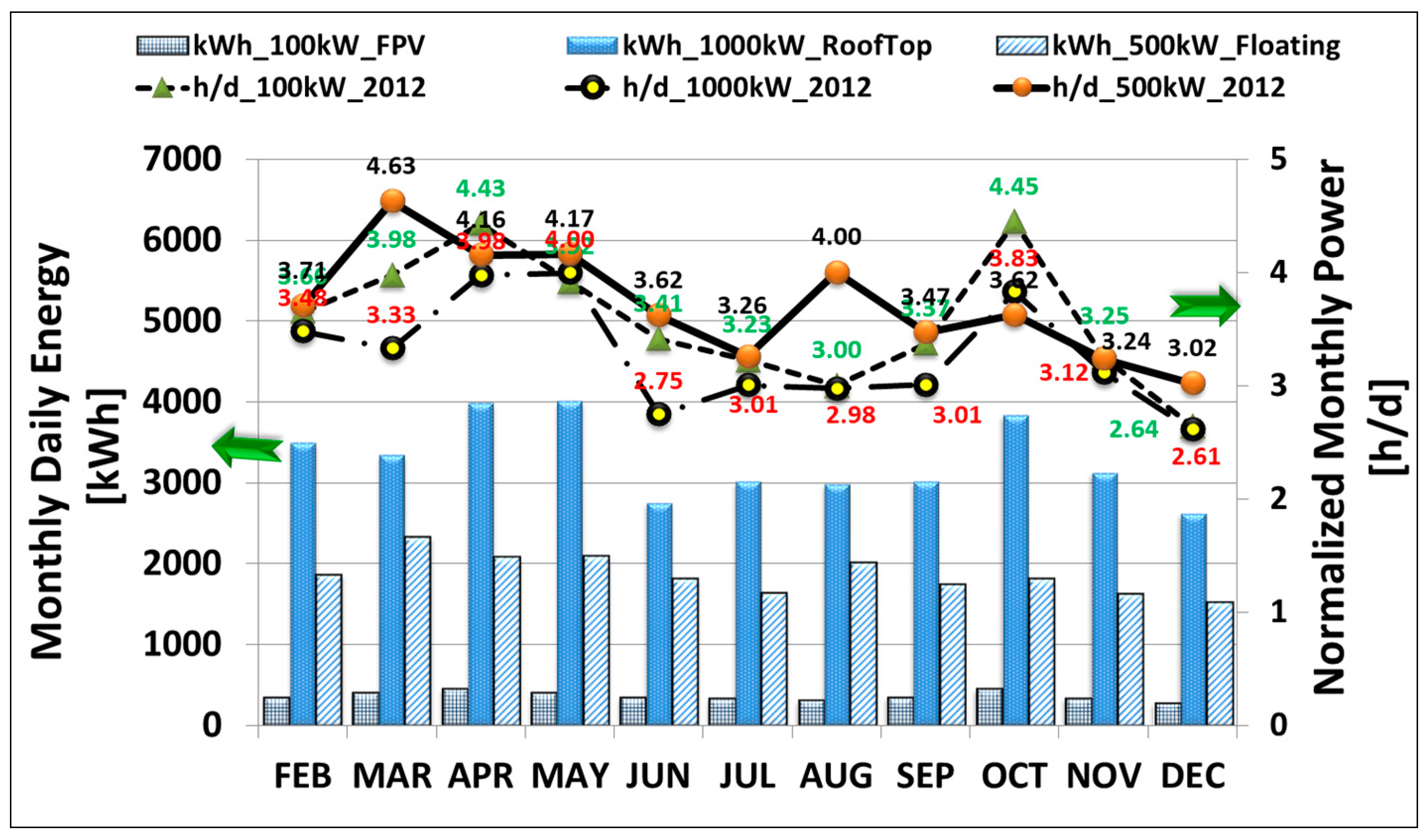
Figure 3.
Predicted versus measured PV module temperature data (100 kW PV system).

Figure 4.
Annual energy generated over module temperature of floating PV temperatures.

Figure 5.
PV predicted cell/module temperature verses ambient temperature (a) and irradiance (b).

Figure 6.
Histograms comparison of FPV Model 1 (a), Model 2 (b), Minitab data fitting model (c), and module field data (d).
Figure 6.
Histograms comparison of FPV Model 1 (a), Model 2 (b), Minitab data fitting model (c), and module field data (d).

Figure 7.
3D surface plots of Model 1 efficiency/Ta/Gt.

Figure 8.
(a) Time series plot of module efficiency (Model 1); (b) efficiency over module temperature.
Figure 8.
(a) Time series plot of module efficiency (Model 1); (b) efficiency over module temperature.


Table 1.
Main sensor specifications.
| Sensor Type | Maker | Model | Accuracy | Range | Mounting |
|---|---|---|---|---|---|
| Solar Irradiance | Apogee | SP-110 | ±5% | 0–1750 Wm2 | Leveling fixture |
| Anemometer (Wind Speed) | Jinyang | WM-IV-WS | ±0.15 m/s | 0–75 m/s | Pole mount |
| Accelerometer | Das | MSENS-IN360 | 0.10° | 0–360° | Pole mount |
| Humidity and Temperature Probe | Vaisala | HMP155 | ±0.176% | −80–60 °C | Protective housing |
| PVM Temperature | Taeyeon | DY-HW-7NN | ±0.20% | −5–55 °C | PVM rear surface |
| Water Temperature | Taeyeon | DY-HW-11NN | ±0.20% | −5–55 °C | Water submerged |
Table 2.
FPVs and rooftop PVs information.
| Project Type | Test Bed | Floating PV | Rooftop PV |
|---|---|---|---|
| Site Name | Hapcheon Dam | Hapcheon Dam | Haman |
| Site Coordinates | N 35.5°33′06″ E 128°00′49″ | N 35.5°33′36″ E 128°02′ 26″ | N 35° 16′10″ E 128° 24′ 01″ |
| Installation Capacity | 100 kW | 500 kW | 1 MW |
| Installation Year | 2011 | 2012 | 2012 |
| Module Slope | 33° | 33° | 30° |
| Module Type | c-Silicon | c-Silicon | c-Silicon |
| Mounting | Aluminum, steel | Aluminum | Aluminum |
| Mounting Type | Fixed | Fixed | Fixed |
| Water Depth | 20 m | 40 m | n/a |
Table 3.
General system performance and output.
| Output Energy | Floating PV | Rooftop PV | ||||
|---|---|---|---|---|---|---|
| 100 kW | 500 kW | 1000 kW | ||||
| Annual Output (kWh/year) | 130,305 | 693,219 | 1,197,547 | |||
| Daily Yearly Average (kWh/year/days of year) | 357 | 1859 | 3281 | |||
| Normal Power | Yearly | kWh/year/kWp | (h/year) | 1303 | 1386 | 1198 |
| Monthly | kWh/month/kWp | (h/month) | Monthly details in Figure 2 | |||
| Daily | kWh/year/days/kWp | (h/d) | 3.58 | 3.80 | 3.28 | |
Table 4.
Multiple regression variables for FPVM temperature (symbol; Tm).
| Term | Predictor Variables | Symbol | Unit |
|---|---|---|---|
| x1 | Ambient Temperature | °C | |
| x2 | Solar Irradiance | W/m² | |
| x3 | Wind Speed | m/s | |
| x4 | Water Temp. | °C |
Table 5.
PV module models.
| Model | Empirical Models |
|---|---|
| Ross (1976) [14] | where |
| Rauschenbach (1980) [15] | |
| Risser & Fuentes (1983) [16] | |
| Schott (1985) [17] | |
| Ross & Smokler (1986) [14] | |
| Mondol et al. (2005, 2007) | |
| Lasnier & Ang (1990) [5] | |
| Servant (1985) | |
| Duffie & Beckman [3] | |
| Koehl (2011) [6] | |
| Kurtz S (2009) [7] | |
| Skoplaki (2009) [8] |
© 2018 by the authors. Licensee MDPI, Basel, Switzerland. This article is an open access article distributed under the terms and conditions of the Creative Commons Attribution (CC BY) license (http://creativecommons.org/licenses/by/4.0/).
Share and Cite
MDPI and ACS Style
Charles Lawrence Kamuyu, W.; Lim, J.R.; Won, C.S.; Ahn, H.K. Prediction Model of Photovoltaic Module Temperature for Power Performance of Floating PVs. Energies 2018, 11, 447. https://doi.org/10.3390/en11020447
AMA Style
Charles Lawrence Kamuyu W, Lim JR, Won CS, Ahn HK. Prediction Model of Photovoltaic Module Temperature for Power Performance of Floating PVs. Energies. 2018; 11(2):447. https://doi.org/10.3390/en11020447
Chicago/Turabian StyleCharles Lawrence Kamuyu, Waithiru, Jong Rok Lim, Chang Sub Won, and Hyung Keun Ahn. 2018. "Prediction Model of Photovoltaic Module Temperature for Power Performance of Floating PVs" Energies 11, no. 2: 447. https://doi.org/10.3390/en11020447
Note that from the first issue of 2016, this journal uses article numbers instead of page numbers. See further details here.