An Improved Rate-Transient Analysis Model of Multi-Fractured Horizontal Wells with Non-Uniform Hydraulic Fracture Properties

Abstract

Although technical advances in hydraulically fracturing and drilling enable commercial production from tight reservoirs, oil/gas recovery remains at a low level. Due to the technical and economic limitations of well-testing operations in tight reservoirs, rate-transient analysis (RTA) has become a more attractive option. However, current RTA models hardly consider the effect of the non-uniform production on rate decline behaviors. In fact, PLT results demonstrate that production profile is non-uniform. To fill this gap, this paper presents an improved RTA model of multi-fractured horizontal wells (MFHWs) to investigate the effects of non-uniform properties of hydraulic fractures (production of fractures, fracture half-length, number of fractures, fracture conductivity, and vertical permeability) on rate transient behaviors through the diagnostic type curves. Results indicate obvious differences on the rate decline curves among the type curves of uniform properties of fractures (UPF) and non-uniform properties of fractures (NPF). The use of dimensionless production integral derivative curve magnifies the differences so that we can diagnose the phenomenon of non-uniform production. Therefore, it’s significant to incorporate the effects of NPF into the RDA models of MFHWs, and the model proposed in this paper enables us to better evaluate well performance based on long-term production data.

1. Introduction

With the depletion of conventional oil/gas resources, tight oil and gas reservoirs have attracted great attention and become significant sources of hydrocarbon supply [1,2,3,4,5,6]. Multistage hydraulically fracturing treatments generate complex fracture networks, which enables commercial production from tight formations [7,8,9,10,11]. However, oil/ gas recovery remains at a low level, even with technical advances in drilling, completion and hydraulic fracturing [12,13,14,15,16,17]. Production rates in tight reservoirs decline quickly after a short period of high production [18]. How to effectively evaluate production performance has become a significant challenge [19,20,21]. Production logging tests (PLTs) are an effective tool to measure the downhole production profile. However, they are expensive and hard to conduct because of complicated downhole situations [12].

Pressure-transient analysis (PTA) and RTA have been acknowledged as effective approaches to understand the reservoir/well performance and estimate its parameters by using transient bottomhole-pressure (BHP) data or long-term production data [22,23,24,25,26,27]. However, due to technical and economic difficulties of well-testing operations in tight reservoirs, RTA based on daily production data is more attractive [23].

In the past decades, empirical methods (e.g., traditional Arps decline-curve) and analytical models (e.g., type curves, straight-line analysis, analytical simulation) have been proposed to interpret reservoir, wellbore and fracture information based on transient rate data. Arps first presented an empirical production correlation to match the rate history and predict future performance during the boundary-dominated flow regime [28]. Fetkovich extended Arps’ work by introducing transient-flow equations into rate decline analysis in the radial-flow system similar with PTA, and further developed a set of type curves for decline curve analysis [29,30]. Chen and Teufel expanded the Fetkovich’s curves to cover the linear-flow condition [31]. The limitation of the methods mentioned above is that they all assume the well pressure solution to be constant [23]. Blasingame et al. defined the normalized rate and how to deal with transient flowing BHP and the variation of gas properties with pressure [32]. Based on Blasingame’s work, Agarwal et al. established the A-G rate-decline analysis type curves to reduce the multiplicity of interpretation by introducing the dimensionless definition of parameters similar with well testing [33]. Some works investigated rate decline analysis for the wells with long period of linear flow (mainly for the vertically fractured well) [34,35]. Badazhkov et al. presented a method for elliptical regime analysis since it is hard to reach pseudo-radial flow in tight reservoirs [36]. The empirical methods have been developed to address the limitations of the Arps curves. Kupchenko et al. extended the traditional Arps curves into tight gas reservoir by considering long-term transient flow [37]. Sarisittitham and Jamiolahmady analyzed the application of Fetkovich-type curves in tight gas and gas condensate reservoirs [23]. However, the application of traditional approaches to unconventional oil/gas reservoirs may lead to uncertainty in production prediction [5]. Recently, many RTA methods have been developed or modified to account for tight gas [23,37,38,39], tight oil [40], shale gas [33,41,42,43,44,45,46,47], etc. Uzun et al. conducted multi-phase RTA in unconventional reservoirs [2]. Integrated approaches are also applied to estimate the parameters and forecast production, such as the combination of analytical and empirical methods [5], the integration of straight-line analysis, type curves and reservoir simulation [39].

However, these researches hardly investigated the effect of the non-uniform production along horizontal wellbore (NPHW) on rate transient behaviors. In fact, PLT results have demonstrated that the production profile is non-uniform [12,48,49] as shown in Figure 1. Although He et al. and Qin et al. [49,50,51] have presented PTA models of to analyze the effects of non-uniform production on pressure transient characteristics, the well testing interpretation is limited since is hard to reflect the information for a large region with testing data due to the low permeability in tight formations and short testing time. Qin et al. discussed the rate transient response of a multi-segment horizontal well with non-uniform production distribution along horizontal wellbores [52]. However, RTA models considering the effect of NPHW are not found. The application of current RTA models of MFHWs may lead to inaccurate interpretation.

Therefore, this work presents an improved RTA model of MFHWs, and the combined type curves are developed to investigate the effects of non-uniform properties of hydraulic fractures on transient rate behaviors in detail. More accurate and reliable results could be achieved through novel models based on long-term production data.

2. RTA Model

The transient production solution under constant pressure condition can be obtained on the basis of transient pressure solution under constant production condition [53]. Therefore, we first derive the transient pressure response of an MFHW in the closed circular reservoir. Then, the production solution can be developed base on the superposition principle.

2.1. Physical Model

The physical model of an MFHW is shown in Figure 2. To derive the practical solution, the following assumptions are taken into account:

(1)

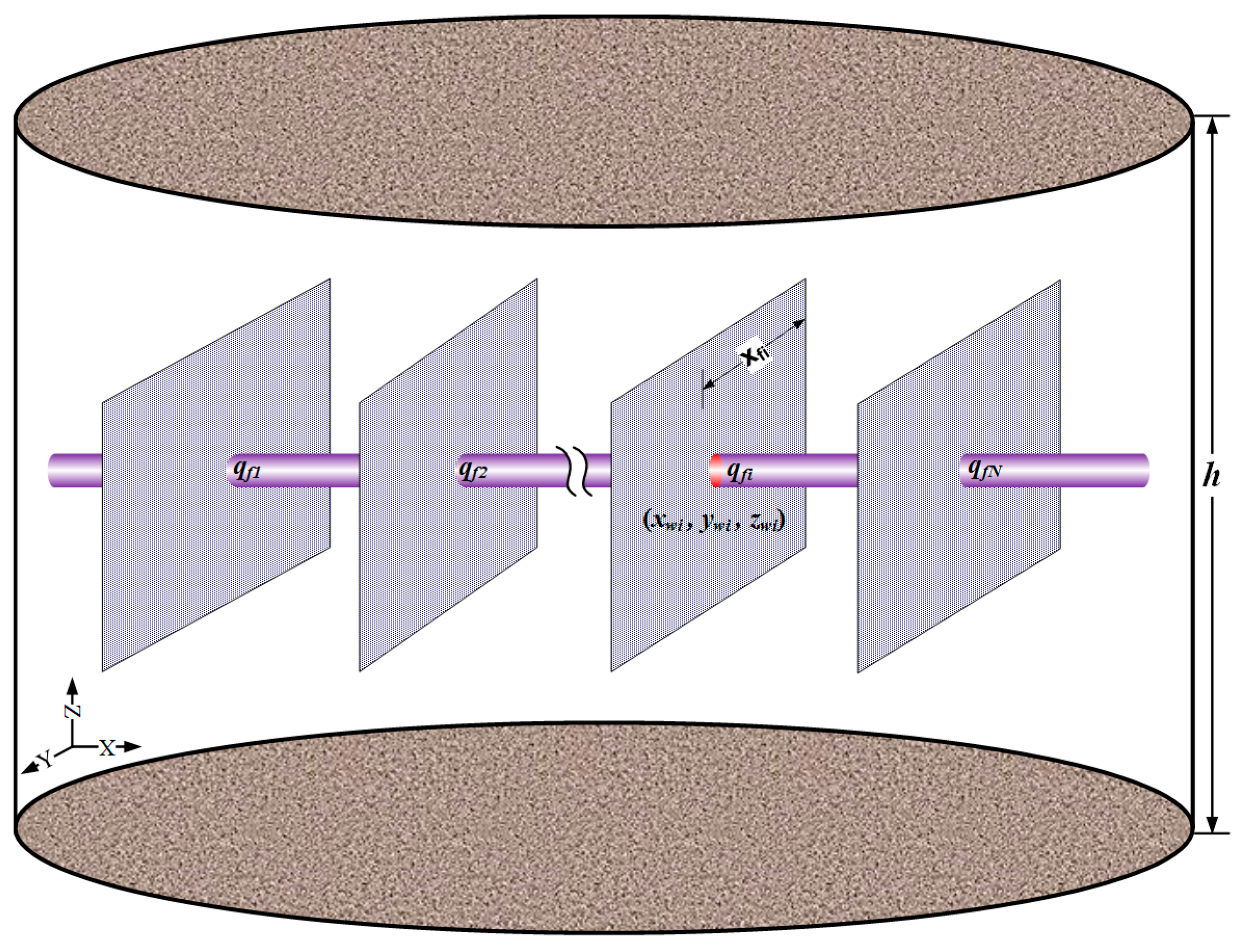
An MFHW is located at a circular-bounded formation with constant thickness (h), porosity (ϕ), total compressibility (C_t), and initial reservoir pressure ($p_i$).

(2)

The horizontal well, with the length of L, is non-uniformly intercepted by multiple fractures. The formation is fully penetrated by hydraulic fractures with half-length (x_f), height (h_f) and width (w_f).

(3)

The formation is considered to be anisotropic and homogeneous. k_h and k_v represent for the permeability in horizontal and vertical direction respectively.

(4)

The formation is saturated with single-phase fluid, and total rates (q) are from fractures in the tight reservoir.

(5)

The effects of capillary pressure and gravity can be ignored.

2.2. Mathematical Model

Based on the derivation in Appendix A, the dimensionless pressure drops of an MFHW with finite conductivity fracture can be obtained through Equations (A11) and (A12):

$$\begin{array}{ll}{P}_D(t_D)& ={\displaystyle \sum _{i=1}^n\left\{\frac{\sqrt{\pi }{q}_{fDi}}{2x_{fDi}}\cdot {\displaystyle {\int }_0^{t_D}\frac{\exp \left[-\frac{{(x_D-x_{wiD})}^2}{4{\tau }_D}\right]}{\sqrt{4{\tau }_D}}}\cdot \left[\mathrm{erf}\left(\frac{x_{fDi}+y_D-y_{wD}}{\sqrt{4{\tau }_D}}\right)+\mathrm{erf}\left(\frac{x_{fDi}-y_D+y_{wD}}{\sqrt{4{\tau }_D}}\right)\right]d{\tau }_D\right\}}\\ & +{\displaystyle \sum _{i=1}^n\left\{\frac{q_{fDi}}{C_{fDi}}\cdot \left[\frac{\pi \cdot {\left(2x_{fi1D}-h_D\right)}^2}{8x_{fDi}}+h_D\cdot \ln \frac{h_D}{2r_{wD}}\right]\right\}}\end{array}$$

(1)

On the basis of the derivation in Appendix B, the pressure solution in Laplace space with incorporating the effects of both skin factor and wellbore storage can be expressed as:

$${\overline{P}}_{wD}(C_D,S,u)=\frac{{\overline{P}}_D+S/\left(u{L}_D\right)}{1+C_{D}uS/L_D+C_D{u}^2{\overline{P}}_D}$$

(2)

The pressure response in the circular-bounded formation can be obtained using the superposition principle:

$${\left(\overline{P_{wD}}\right)}_{boundary}={\left(\overline{P_{wD}}\right)}_{infinite}+{\left(\overline{P_{wD}}\right)}_{closedcircularboundary}$$

(3)

where ${\left(\overline{P_{wD}}\right)}_{boundary}$ means the pressure solution of an MFHW in circular-bounded formation. ${\left(\overline{P_{wD}}\right)}_{infinite}$ denotes the pressure in which the formation is infinite in horizontal direction and impermeable in vertical direction. ${\left(\overline{P_{wD}}\right)}_{closed circular boundary}$ represents for the pressure response caused by the circular-bounded formation.

The effect of closed circular boundary on pressure response can be calculated by [30]:

$${\left({\overline{P}}_{wD}\right)}_{closedcircularboundary}=\frac{1}{u}\frac{1}{\sqrt{u}}\frac{K_1\left(\sqrt{u}{r}_{eD}\right)}{I_1\left(\sqrt{u}{r}_{eD}\right)}{\displaystyle {\int }_0^{\sqrt{u}}{I}_0\left(z\right)dz}$$

(4)

Therefore, the final pressure solution of an MFHW in the circular-bounded formation can be expressed as:

$${\left(\overline{P_{wD}}\right)}_{boundary}=\frac{{\overline{P}}_D+S/\left(u{L}_D\right)}{1+C_{D}uS/L_D+C_D{u}^2{\overline{P}}_D}+\frac{1}{u}\frac{1}{\sqrt{u}}\frac{K_1\left(\sqrt{u}{r}_{eD}\right)}{I_1\left(\sqrt{u}{r}_{eD}\right)}{\displaystyle {\int }_0^{\sqrt{u}}{I}_0\left(z\right)dz}$$

(5)

2.3. Solution Approach

${\overline{P}}_{wD}$ can be inverted into real space by the Stehfest inversion algorithm [54]. According to the Laplace transformation and Duhamel’s Principle, the production solution under constant pressure in Laplace space can be achieved based on the pressure solution under constant production conditions [53]:

$${\overline{q}}_D\left(u\right)=\frac{1}{u^2{\left(\overline{P_{wD}}\right)}_{boundary}}$$

(6)

Blasingame et al. [35] defined three parameters to better reflect the rate transient behaviors:

$$q_{Dd}=q_D\cdot b_{Dpss}$$

(7)

$$q_{Ddi}=\frac{1}{t_{Dd}}{\displaystyle {\int }_0^{t_{Dd}}{q}_{Dd}\left(\tau \right)}d\tau$$

(8)

$$q_{Ddid}=-\frac{d{q}_{Ddi}}{d\ln t_{Dd}}=-t_{Dd}\frac{d{q}_{Ddi}}{d{t}_{Dd}}$$

(9)

where q_Dd denotes the normalized dimensionless decline rate, q_Ddi represents for the normalized dimensionless decline rate integral, and q_Ddid is the normalized dimensionless decline rate integral derivative. t_Dd is the dimensionless decline time. The dimensionless material balance time function (t_cDd) can be calculated by:

$$t_{cDd}=\frac{t_{cD}}{0.5(r_{eD}^2-1)b_{Dpss}}=\frac{k/\left(\varphi \mu C_t\right)\cdot t_c\cdot x_f^2}{0.5(r_{eD}^2-1)b_{Dpss}}$$

(10)

The introduction of q_Ddi and q_Ddid amplify the rate transient characteristics and make production data easier to analyse.

3. Combined Type Curve

The combined type curves are developed, including the normalized dimensionless decline rate curve (q_Dd), the normalized dimensionless decline rate integral curve (q_Ddi), and the normalized dimensionless decline rate integral derivative curve (q_Ddid). To investigate the effect of fracture properties on rate decline characteristics, we develop the type curves of uniform properties of fractures (UPF) and nonuniform properties of fractures (NPF) respectively. The constant parameters for all cases in this work can be found in

Table 1. The basic parameters of reservoir and MFHWs (constant for Figures 1–9).

Parameters	Value
Thickness of formation (h)	20.0 × 102 cm
Permeability in the horizontal direction (kh)	1.0 × 10−3 D
Permeability in the horizontal direction (kv)	0.1 × 10−3 D
Length of horizontal wellbore (L)	1200 × 102 cm
Radius of horizontal wellbore (rw)	0.1 × 102 cm
Dimensionless wellbore-storage coefficient (CD)	2 × 10−5
Skin factor (S)	1.0

.

The parameters of hydraulic fractures are shown in

Table 2. The basic parameters of hydraulic fractures.

Parameters	Value
	Case1 (UPF)	Case 2 (NPF)
Number of fractures (n)	4
Dimensionless fracture half-length (xfD)	0.05:0.05:0.05:0.05	0.09:0.01:0.01:0.09
Dimensionless production of fractures (qfD)	0.25:0.25:0.25:0.25	0.48:0.02:0.02:0.48
Dimensionless fracture conductivity (CfD)	0.50:0.50:0.50:0.50	0.90:0.10:0.10:0.90

. The total production, fracture half-length, and fracture conductivity keep the same for two cases. There also exist differences in fracture parameters between Case 1 and Case 2. In Case 1, all fractures have the same half-length, production rate, and conductivity. But the production rate of fractures with longer half-length and higher conductivity are higher than those with shorter half-length and lower conductivity in Case 2.

To compare the type curves of two cases, the combined type curves under UPF and NPF are included in the same figure, shown in Figure 3. The green lines represent for the normalized dimensionless decline production integral curve (q_Ddi). The yellow lines denote the normalized dimensionless decline production curves (q_Dd). The purple curves are the dimensionless decline production integral derivative curve (q_Ddid). Obvious differences can be found between UPF (the solid lines) and NPF (the dotted lines) especially before the boundary-dominated flow regime. In Case 2, the interferences among fractures are much smaller than Case 1. The use of dimensionless production integral derivative curve magnifies the differences so that we can diagnose the phenomenon of non-uniform production. Hence, it’s necessary to consider the effect of NPF into the RDA models of MFHWs to better evaluate well performance.

4. Sensitivity Analysis

The comparisons of type curves indicate that the effect of NPF cannot be ignored. Here, we will discuss the effect of fracture parameters on rate transient behaviors in detail, including fracture half-length, production of hydraulic fractures, number of hydraulic fractures, and fracture conductivity.

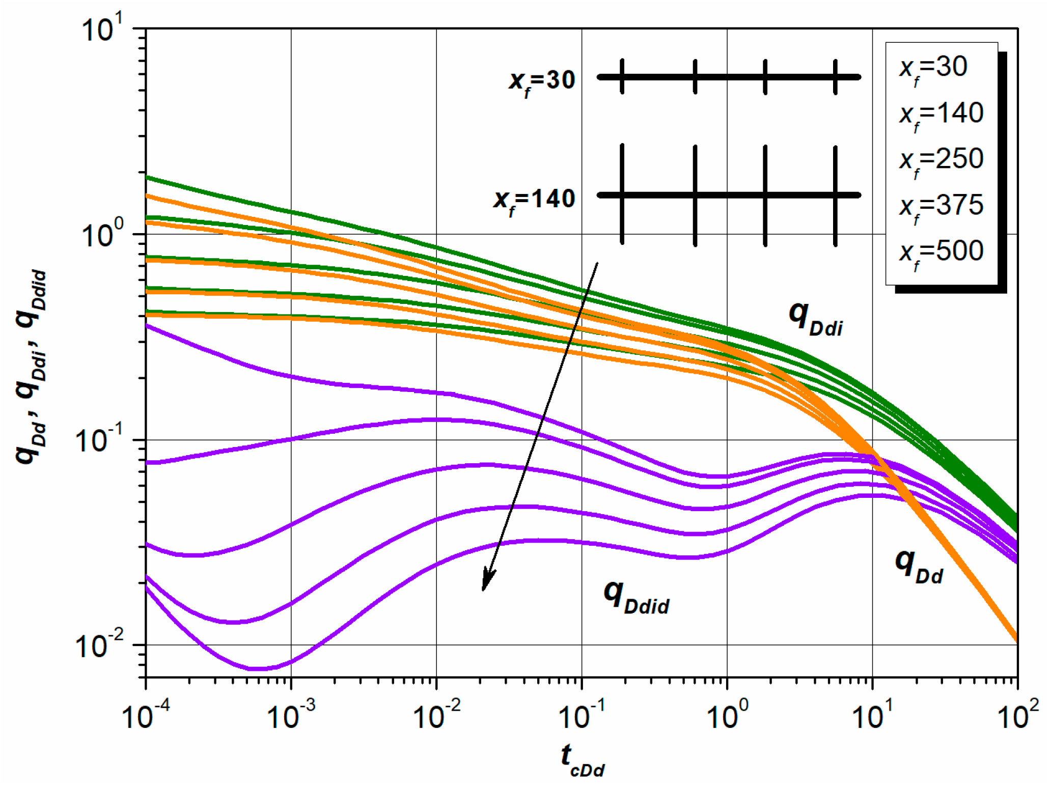
4.1. Fracture Half-Length

Two kinds of cases are designed. The fundamental parameters can also be found in Table 1. The half-length of individual fracture (x_fD) is equal while the total lengths of fractures are different for Case 1. Additionally, the production and conductivity of each fracture are equal, and the total production and conductivity of all fractures keep the same in the first case. The combined type curves are shown in Figure 4. The x_fD is 0.03, 0.14, 0.25, 0.40, and 0.50, respectively, as shown in Figure 4. The total fracture length makes a big difference on production performance. With the increase of fracture length, the combined curves move down, especially during the transient flow regime. Longer fracture lengths means bigger hydraulic scale and more intense interferences among fractures under the same number of fractures. It makes data more disperse through the dimensionless production integral derivative. Through the three curves, the facture half-length can be estimated based on the production data.

In Case 2, the half-length of individual fracture (x_fD) is unequal, and the total length of fractures keep the same. Other parameters keep the same as that in Case 1. The half-length of different fractures are shown in Figure 5. Although the effects of unequal half-length of fractures on type curves are not obvious compared to Case 1, the use of the production integral derivative curves magnify the differences. Through the comparison between Case 1 and Case 2, we can conclude that total length of fractures affects the rate decline behaviors more obviously than unequal half-length of fractures with the same total length of fractures since interferences between fractures influence the rate transient characteristics a lot.

4.2. Production of Hydraulic Fractures

Five cases are chosen to analyze the effects of production rate of different fractures on type curves (q_fD = 0.10:0.10:0.40:0.40; 0.10:0.40:0.40:0.10; 0.25:0.25:0.25:0.25:0.25; 0.40:0.40:0.10:0.10). The total production rates are the same for all cases. The basic parameters are shown in Table 1, and other parameters of fracture are the same. Figure 6 shows the combined type curves of an MFHW with different kinds of production distribution along horizontal wellbore. Big differences can be observed among uniform and non-uniform production distribution along horizontal wellbores, especially during the transient flow period. With the increase of the production from the fractures near the heel of horizontal wellbore, three kinds of curves move down. Symmetric distribution of production (i.e., q_fD = 0.10:0.10:0.40:0.40; q_fD = 0.40:0.40:0.10:0.10) generates different results so that this model can be used to distinguish the symmetric cases. Additionally, the differences during the boundary-dominated flow regime can be identified on the production integral derivative curves. Therefore, the production profile can be diagnosed through the model proposed in this paper.

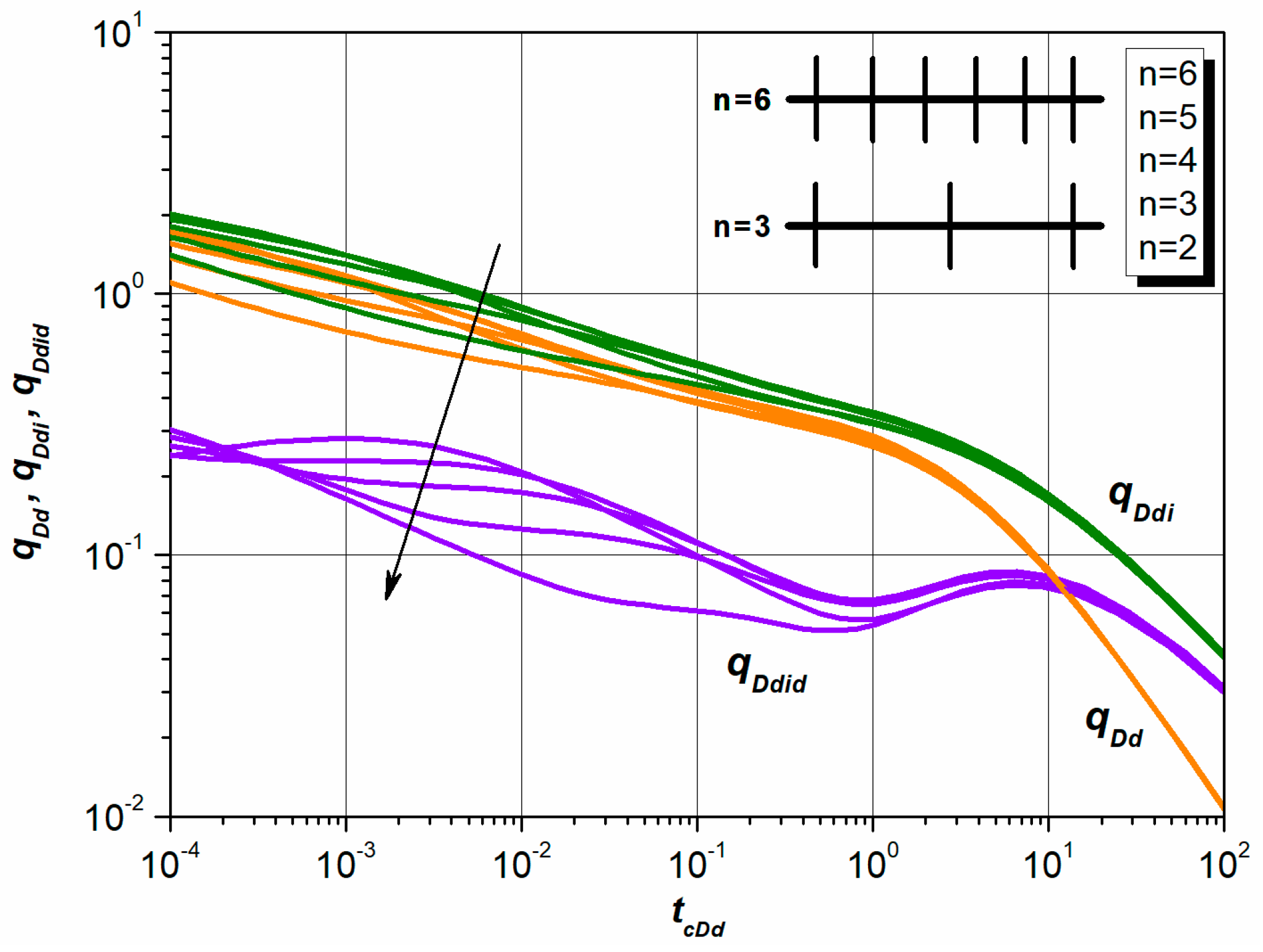
4.3. Number of Hydraulic Fractures

Five cases are chosen to analyze the effects of number of fractures on type curves (n = 2, 3, 4, 5, 6). Other fracture parameters remain the same. Three kinds of curves move up with the increase of number of fractures, shown in Figure 7. Obvious differences can be found on the dimensionless production integral derivative curves during the middle transient flow period. The number of fractures can be estimated on the basis of long-term production data.

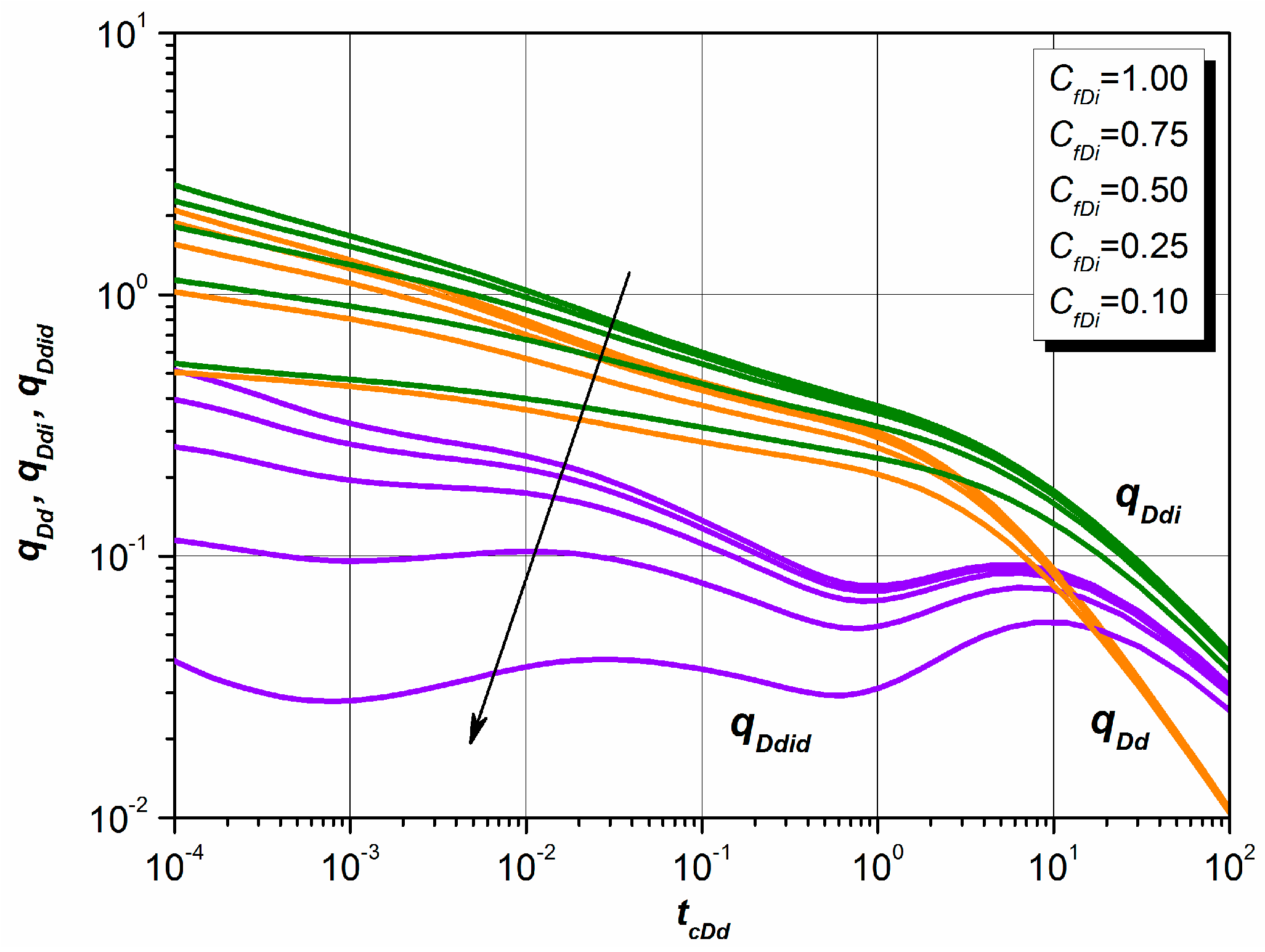
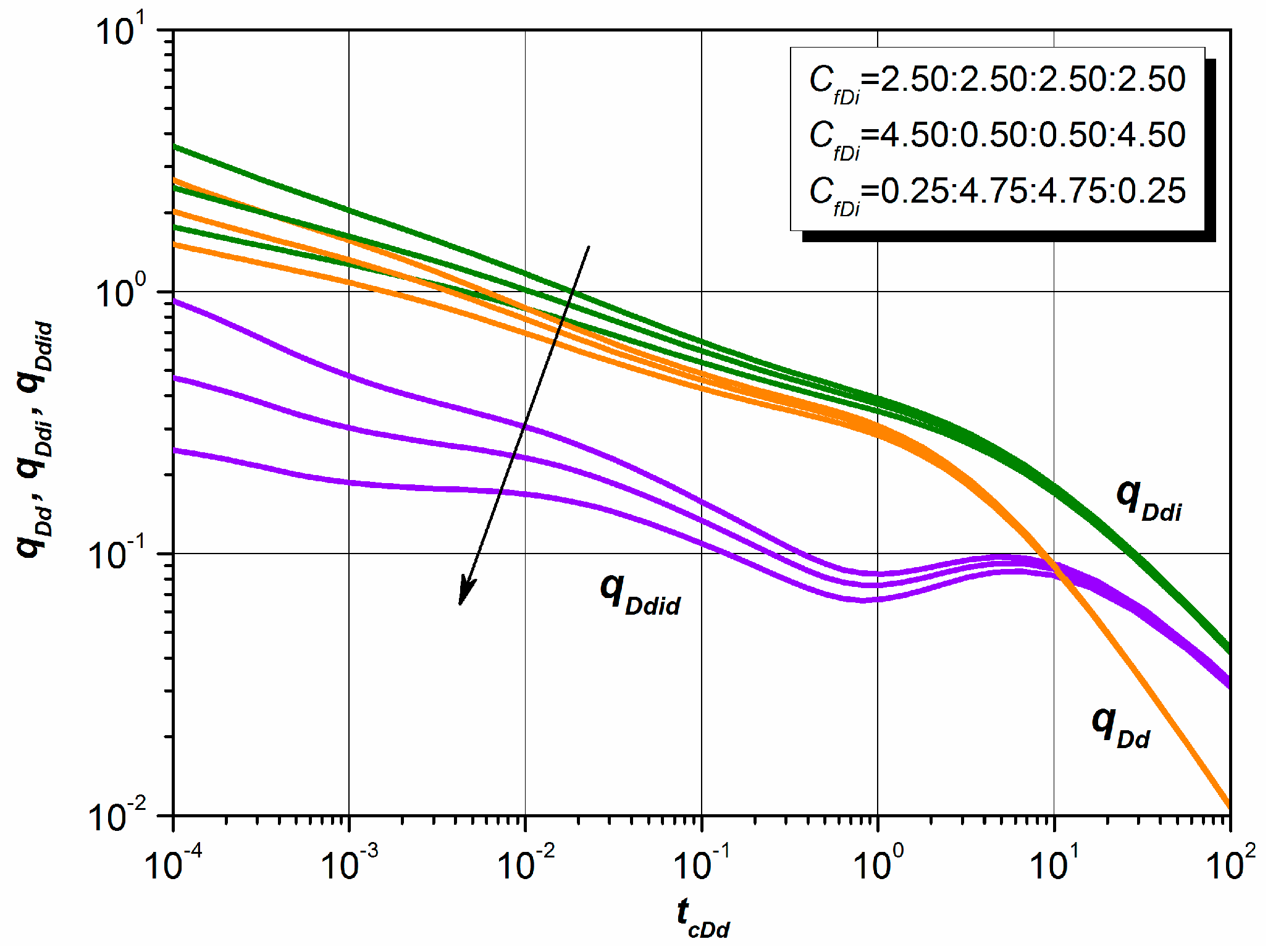
4.4. Fracture Conductivity

In order to discuss the influences of fracture conductivity on rate transient response, two cases are analyzed. In Case 1, the total conductivity of fractures are different while the conductivity of individual fracture is equal. The C_fD equals to 0.10, 0.25, 0.50, 0.75, and 1.00 respectively. Other parameters keep the same. It is observed that the fracture conductivity is a significant factor for rate decline behaviors as shown in Figure 8. The combined type curves move down with the decrease of fracture conductivity. This is because lower conductivity result in higher pressure drop so that the dimensionless production also becomes lower. The effects of facture conductivity on type curves decrease when C_fD is larger than 1.0.

Due to the differences of fracturing scale, formation damage, etc., the conductivity of each fracture is not the same in fact. Three examples are designed to analyze the effect of non-uniform fracture conductivity on rate transient behaviors in Case 2 (i.e., C_fDi = [4.5 0.5 0.5 4.5]; C_fDi = [2.5 2.5 2.5 2.5]; C_fDi = [0.25 4.75 4.75 0.25]). The total conductivity keeps the same for three examples. There are obvious differences between uniform and non-uniform fracture conductivity, shown in Figure 9. Because the reference point is considered as the heel of horizontal wellbore, low fracture conductivity of fractures near the heel of horizontal wellbore bring about high pressure drops, leading to smaller dimensionless production. Thus, the combined curves move down with decreasing the conductivity of fracture near the heel of horizontal wellbore. Therefore, the effect of non-uniform fracture conductivity on rate behaviors should not be neglected.

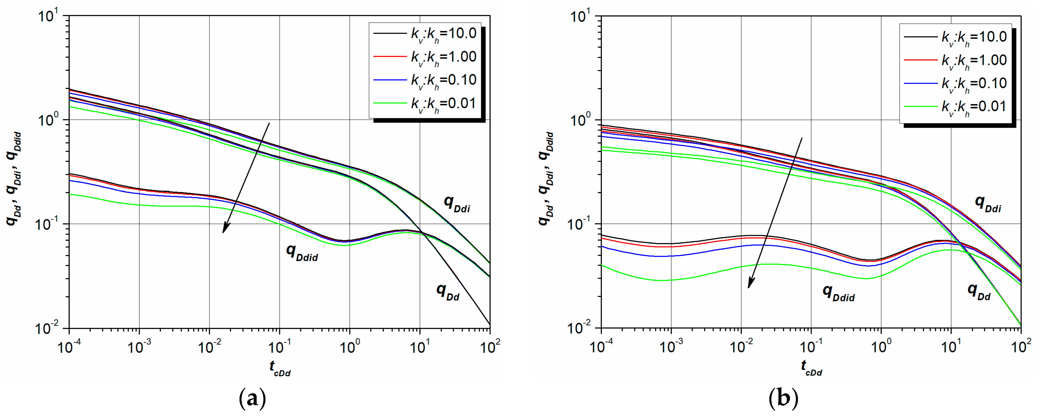
4.5. Ratio of Vertical Permeability to Horizontal Permeability

To analyze the effect of vertical permeability on rate decline characteristics, eight cases are divided into two groups. The formation thickness of two groups are 20 m and 100 m respectively. Different ratios of vertical permeability to horizontal permeability are used to generate the corresponding rate response (k_v:k_h = 0.01:0.10:1.00:10.0). Other parameters are kept the same for the eight cases. Combined type curves move down with the decrease of ratio of vertical permeability to horizontal permeability as shown in Figure 10. The influence of vertical permeability may be reduced when formation thickness decreases. When formation thickness equals to 20 m, the differences are not obvious under different ratio of vertical permeability to horizontal permeability, shown in Figure 10a. With the increase of formation thickness (e.g., h = 100 m), the differences become obvious as shown in Figure 10b. Using dimensionless production integral derivative curve enables us to better distinguish the influences of different vertical permeability on type curves.

5. Conclusions

This paper presents an improved RTA model of MFHWs in the circular-closed formation, and further develops the combined type curves. Here are the conclusions and suggestions obtained from this work.

(1)

The production distribution along horizontal wellbore is non-uniform, and the properties of different fractures are also unequal, which should be taken into account in the RTA model and later interpretation.

(2)

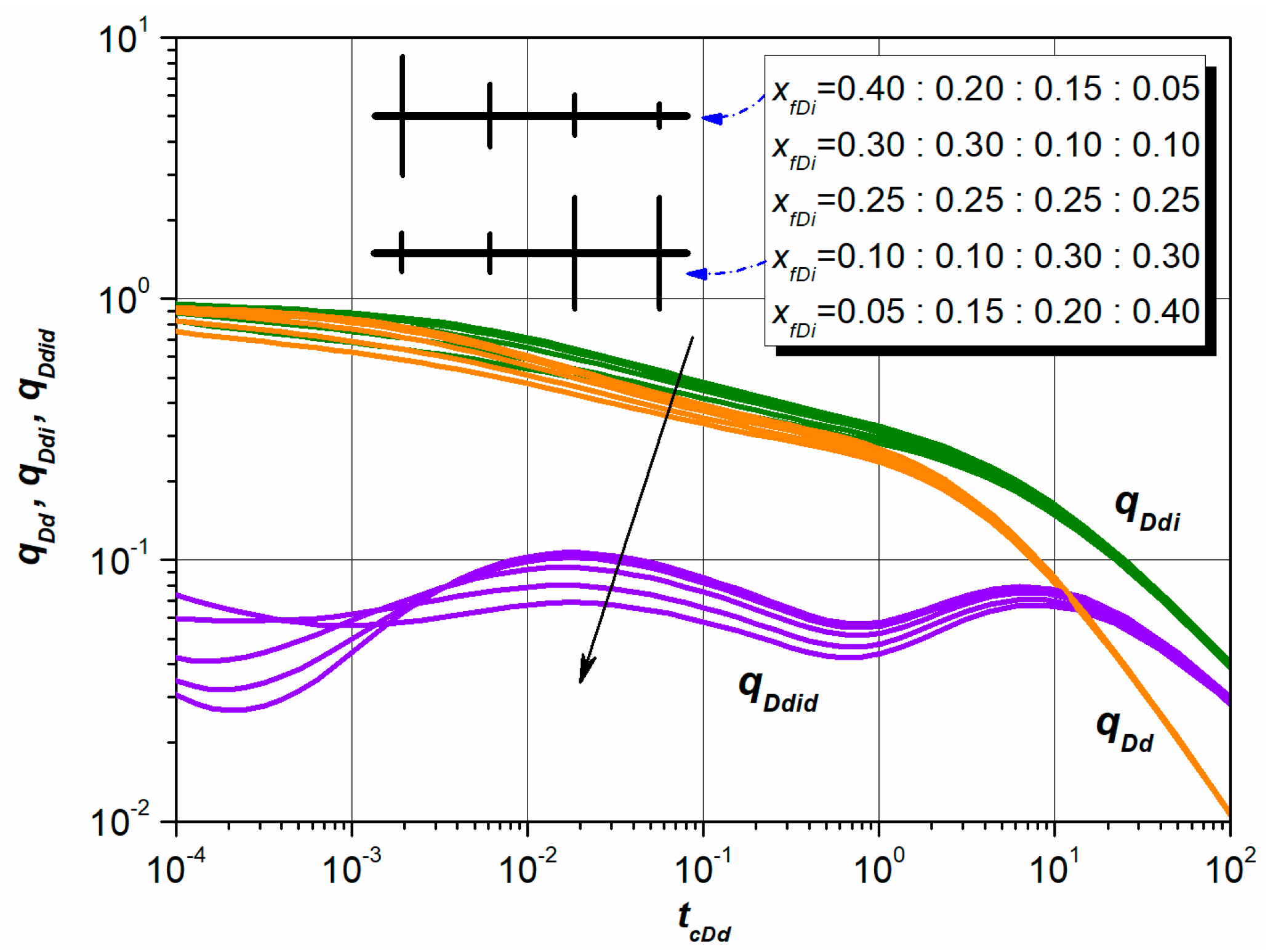
Although the effects of unequal half-length of fractures on type curves are not obvious, the use of the use of dimensionless production integral derivative curve magnifies the differences so that we can identify the production distribution.

(3)

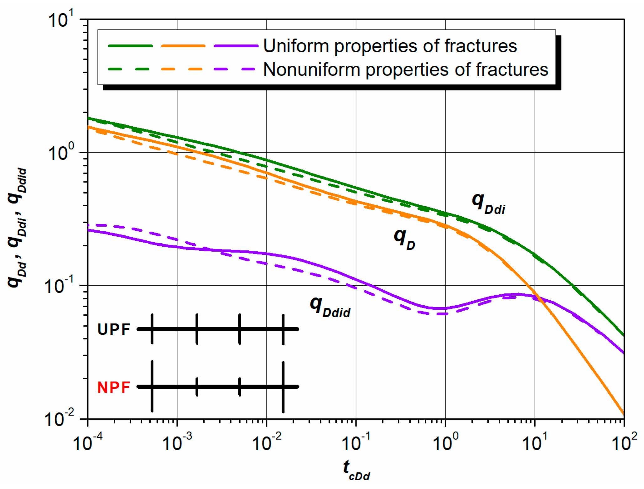
Obvious differences can be observed among the type curves of UPF and NPF. Total length of fractures affects the rate decline behaviors more obviously than unequal half-length of fractures with same total length of fractures.

(4)

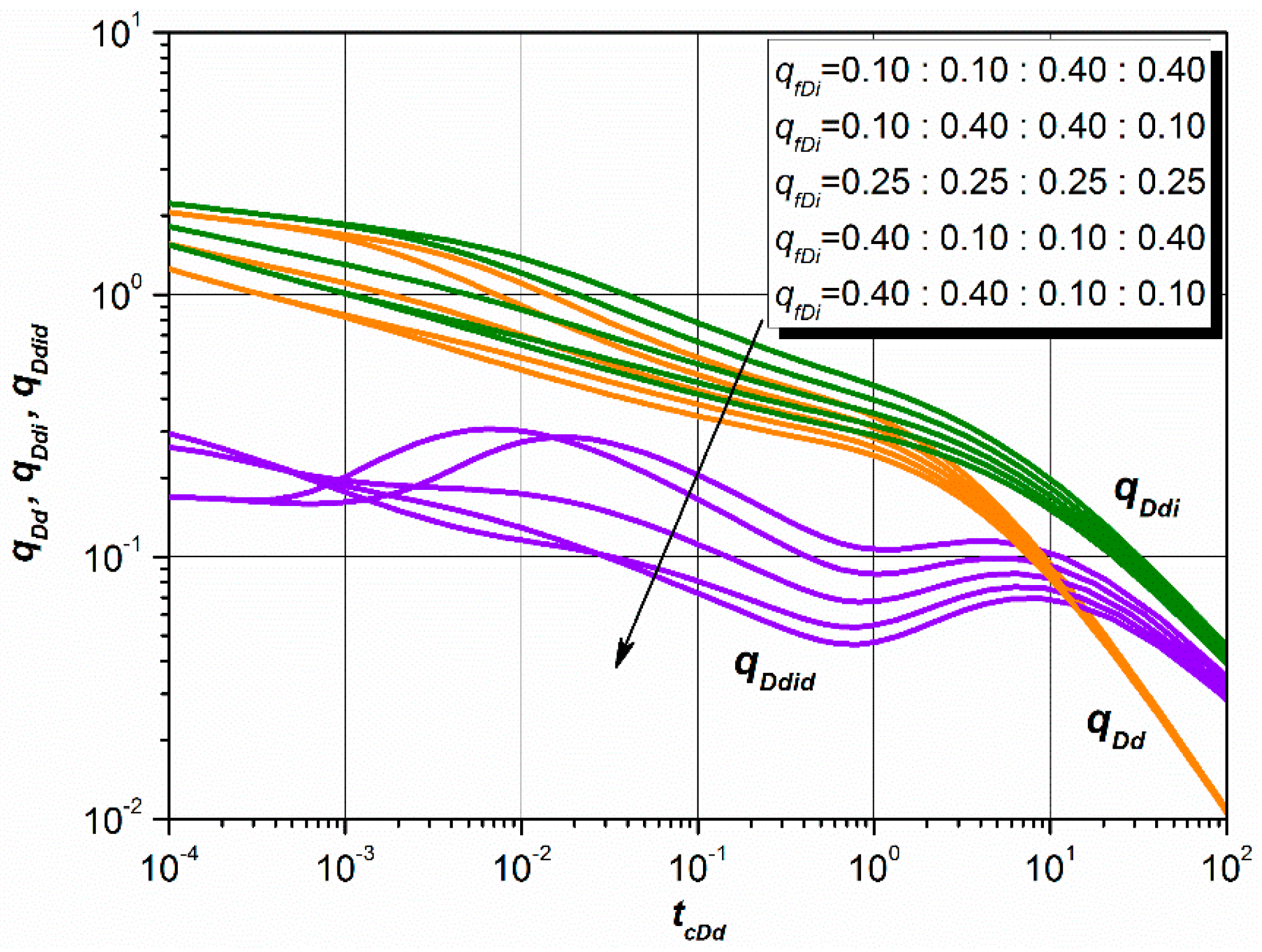
Since the reference point locates at the heel of horizontal wellbore, symmetric distribution of production (i.e., q_fD = 0.10:0.10:0.40:0.40; q_fD = 0.40:0.40:0.10:0.10) generates different results so that this model can be used to distinguish the symmetric cases.

In conclusion, the proposed RTA model enables petroleum engineers to better evaluate production performance of MFHWs, and interpret reservoir and well parameters more accurately based on dynamic long-term production data.

References

1. Clarkson, C.R. Production Data Analysis of Unconventional Gas Wells: Review of Theory and Best Practices. Int. J. Coal Geol. 2013, 109, 101–146. [Google Scholar] [CrossRef]
2. Uzun, I.; Kurtoglu, B.; Kazemi, H. Multiphase Rate-Transient Analysis in Unconventional Reservoirs: Theory and Application. SPE Reserv. Eval. Eng. 2016, 19, 553–566. [Google Scholar] [CrossRef]
3. Wang, L.; Wang, S.; Zhang, R.; Rui, Z. Review of Multi-Scale and Multi-Physical Simulation Technologies for Shale and Tight Gas Reservoir. J. Nat. Gas Sci. Eng. 2017, 37, 560–578. [Google Scholar] [CrossRef]
4. Cui, G.; Ren, S.; Rui, Z.; Ezekiel, J.; Zhang, L.; Wang, H. The influence of complicated fluid-rock interactions on the geothermal exploitation in the CO2 plume geothermal system. Appl. Energy 2018. [Google Scholar] [CrossRef]
5. Clarkson, C.R. Production Data Analysis of Unconventional Gas Wells: Workflow. Int. J. Coal Geol. 2013, 109, 147–157. [Google Scholar] [CrossRef]
6. Rui, Z.; Han, G.; Zhang, H.; Wang, S.; Pu, H.; Ling, K. A new model to evaluate two leak points in a gas pipeline. J. Nat. Gas Sci. Eng. 2017, 46, 491–497. [Google Scholar] [CrossRef]
7. Chai, Z.; Yan, B.; Killough, J.E.; Wang, Y. Dynamic Embedded Discrete Fracture Multi-Continuum Model for the Simulation of Fractured Shale Reservoirs. In Proceedings of the International Petroleum Technology Conference, Bangkok, Thailand, 14–16 November 2016; International Petroleum Technology Conference: Richardson, TX, USA, 2016. [Google Scholar]
8. Sun, J.; Gamboa, E.; Schechter, D.; Rui, Z. An Integrated Workflow for Characterization and Simulation of Complex Fracture Networks Utilizing Microseismic and Horizontal Core Data. J. Nat. Gas Sci. Eng. 2016, 34, 1347–1360. [Google Scholar] [CrossRef]
9. Sun, Z.; Espinoza, D.N.; Balhoff, M.T. Discrete Element Modeling of Indentation Tests to Investigate Mechanisms of CO2-Related Chemomechanical Rock Alteration. J. Geophys. Res. Solid Earth. 2016, 121, 7867–7881. [Google Scholar] [CrossRef]
10. Rui, Z.; Wang, X.; Zhang, Z.; Lu, J.; Chen, G.; Zhou, X.; Patil, S. A realistic and integrated model for evaluating oil sands development with steam assisted gravity drainage technology in Canada. Appl. Energy 2018, 213, 76–91. [Google Scholar] [CrossRef]
11. Tang, H.; Killough, J.E.; Heidari, Z. A New Technique To Characterize Fracture Density by Use of Neutron Porosity Logs Enhanced by Electrically Transported Contrast Agents. SPE J. 2016, 22, 1034–1045. [Google Scholar] [CrossRef]
12. He, Y.; Cheng, S.; Qin, J.; Chen, J.; Wang, Y.; Feng, N.; Yu, H. Successful Application of Well Testing and Electrical Resistance Tomography to Determine Production Contribution of Individual Fracture and Water-Breakthrough Locations of Multifractured Horizontal Well in Changqing Oil Field, China. In Proceedings of the SPE Annual Technical Conference and Exhibition, San Antonio, TX, USA, 9–11 October 2017; Society of Petroleum Engineers: Richardson, TX, USA, 2017. SPE-187285-MS. [Google Scholar] [CrossRef]
13. Qin, J.; Liu, Y.; Feng, Y.; Ding, Y.; Liu, L.; He, Y. New Well Pattern Optimization Methodology in Mature Low-Permeability Anisotropic Reservoirs. J. Geophys. Eng. 2018, 15, 93–105. [Google Scholar] [CrossRef]
14. He, Y.; Cheng, S.; Li, L.; Mu, G.; Zhang, T.; Xu, H.; Qin, J.; Yu, H. Waterflood Direction and Front Characterization with Four-Step Work Flow: A Case Study in Changqing Oil Field, China. SPE Reserv. Eval. Eng. 2017, 20, 708–725. [Google Scholar] [CrossRef]
15. Rui, Z.; Li, C.; Peng, F.; Ling, K.; Chen, G.; Zhou, X. Chang, H. Development of Industry Performance Metrics For Offshore Oil and Gas Project. J. Nat. Gas Sci. Eng. 2017, 39, 44–53. [Google Scholar] [CrossRef]
16. Jing, J.; Sun, J.; Tan, J. Investigation on Flow Patterns and Pressure Drops of Highly Viscous Crude Oil–Water Flows in a Horizontal Pipe. Exp. Therm. Fluid Sci. 2016, 72, 88–96. [Google Scholar] [CrossRef]
17. He, Y.; Cheng, S.; Li, L.; Mu, G.; Zhang, T.; Xu, H.; Qin, J.; Yu, H. Waterflood Direction and Front Characterization with Multiple Methods: A Case Study in Changqing Oilfield, China. In Proceedings of the SPE Oil and Gas India Conference and Exhibition, Mumbai, India, 24–26 November 2015; Society of Petroleum Engineers: Richardson, TX, USA, 2015. SPE-178053-MS. [Google Scholar] [CrossRef]
18. Ren, W.; Li, G.; Tian, S.; Sheng, M.; Geng, L. Adsorption and Surface Diffusion of Supercritical Methane in Shale. Ind. Eng. Chem. Res. 2017, 56, 3446–3455. [Google Scholar] [CrossRef]
19. Rui, Z.; Peng, F.; Ling, K.; Chang, H.; Chen, G.; Zhou, X. Investigation Into The Performance of Oil and Gas Projects. J. Pet. Sci. Eng. 2017, 38, 12–20. [Google Scholar] [CrossRef]
20. Hu, J.; Zhang, C.; Rui, Z.; Yu, Y.; Chen, Z. Fractured horizontal well productivity prediction in tight oil reservoirs. J. Pet. Sci. Eng. 2017, 151, 159–168. [Google Scholar] [CrossRef]
21. Rui, Z.; Lu, J.; Zhang, Z.; Guo, R.; Ling, K.; Zhang, R.; Patil, S. A Quantitative Oil and Gas Reservoir Evaluation System for Development. J. Nat. Gas Sci. Eng. 2017, 42, 31–39. [Google Scholar] [CrossRef]
22. Sarisittitham, S.; Jamiolahmady, M. Decline Curve Analysis for Tight Gas and Gas Condensate Reservoirs. In Proceedings of the International Petroleum Technology Conference, Kuala Lumpur, Malaysia, 10–12 December 2014; International Petroleum Technology Conference: Richardson, TX, USA, 2014. IPTC-18188-MS. [Google Scholar]
23. Zuo, L.; Yu, W.; Wu, K. A fractional decline curve analysis model for shale gas reservoirs. Int. J. Coal Geol. 2016, 163, 140–148. [Google Scholar] [CrossRef]
24. He, Y.; Cheng, S.; Qin, J.; Wang, Y.; Feng, N.; Hu, L.; Huang, Y.; Fang, R.; Yu, H. A semianalytical approach to estimate the locations of malfunctioning horizontal wellbore through bottom-hole pressure and its application in Hudson oilfield. In Proceedings of the SPE Middle East Oil & Gas Show and Conference, Manama, Kingdom of Bahrain, 6–9 March 2017; Society of Petroleum Engineers: Richardson, TX, USA, 2017. SPE-183796-MS. [Google Scholar] [CrossRef]
25. Wang, Y.; Cheng, S.; Feng, N.; He, Y.; Yu, H. The Physical Process and Pressure-Transient Analysis Considering Fractures Excessive Extension in Water Injection Wells. J. Pet. Sci. Eng. 2017, 151, 439–454. [Google Scholar] [CrossRef]
26. Zhang, X.; Wang, X.; Hou, X.; Xu, W. Rate Decline Analysis of Vertically Fractured Wells in Shale Gas Reservoirs. Energies 2017, 10, 1602. [Google Scholar] [CrossRef]
27. Wang, M.; Fan, Z.; Xing, G.; Zhao, W.; Song, H.; Su, P. Rate Decline Analysis for Modeling Volume Fractured Well Production in Naturally Fractured Reservoirs. Energies 2018, 11, 43. [Google Scholar] [CrossRef]
28. Arps, J.J. Analysis of Decline Curves. Pet. Trans. 1945, 160, 228–247. [Google Scholar] [CrossRef]
29. Fetkovich, M.J. Decline Curve Analysis Using Type Curves. J. Pet. Technol. 1980, 32, 1065–1077. [Google Scholar] [CrossRef]
30. Fetkovich, M.J.; Vienot, M.E.; Bradley, M.D.; Kiesow, U.G. Decline Curve Analysis Using Type Curves: Case Histories. SPE Form. Eval. 1987, 2, 637–656. [Google Scholar] [CrossRef]
31. Chen, H.; Teufel, L.W. A New Rate-Time Type Curve for Analysis of Tight-Gas Linear and Radial Flows. In Proceedings of the SPE Annual Technical Conference and Exhibition, Dallas, TX, USA, 1–4 October 2000; Society of Petroleum Engineers: Richardson, TX, USA, 2000. SPE 63094-MS. [Google Scholar]
32. Blasingame, T.A.; McCray, T.L.; Lee, W.J. Decline curve analysis for variable pressure drop/variable flowrate systems. In Proceedings of the SPE Gas Technology Symposium, Houston, TX, USA, 22–24 January 1991; Society of Petroleum Engineers: Richardson, TX, USA, 1991. SPE-21513-MS. [Google Scholar]
33. Agarwal, R.G.; Gardner, D.C.; Kleinsteiber, S.W.; Fussell, D.D. Analyzing Well Production Data Using Combined-Type-Curve and Decline-Curve Analysis Concepts. SPE Reserv. Eval. Eng. 1999, 2, 478–486. [Google Scholar] [CrossRef]
34. Wattenbarger, R.A.; El-Banbi, A.H.; Villegas, M.E.; Maggard, J.B. Production Analysis of Linear Flow into Fractured Tight Gas Wells. In Proceedings of the SPE Rocky Mountain Regional/Low-Permeability Reservoirs Symposium, Denver, CO, USA, 5–8 April 1998; Society of Petroleum Engineers: Richardson, TX, USA, 1998. SPE-39931-MS. [Google Scholar]
35. Pratikno, H.; Rushing, J.A.; Blasingame, T.A. Decline curve analysis using type curves-fractured wells. In Proceedings of the SPE Annual Technical Conference and Exhibition, Denver, CO, USA, 5–8 October 2003; Society of Petroleum Engineers: Richardson, TX, USA, 2003. SPE-84287-MS. [Google Scholar]
36. Badazhkov, D.; Dmitry, O.; Kovalenko, A. Analysis of Production Data with Elliptical Flow Regime in Tight Gas Reservoirs. In Proceedings of the SPE Russian Oil and Gas Technical Conference and Exhibition, Moscow, Russia, 28–30 October 2008; Society of Petroleum Engineers: Richardson, TX, USA, 2008. SPE-117023-MS. [Google Scholar]
37. Kupchenko, C.L.; Gault, B.W.; Mattar, L. Tight Gas Production Performance Using Decline Curves. In Proceedings of the CIPC/SPE Gas Technology Symposium 2008 Joint Conference, Calgary, AB, Canada, 16–19 June 2008; Society of Petroleum Engineers: Richardson, TX, USA, 2008. SPE-114991-MS. [Google Scholar]
38. Ilk, D.; Rushing, J.A.; Perego, A.D.; Blasingame, T.A. Exponential vs. hyperbolic decline in tight gas sands: Understanding the origin and implications for reserve estimates using Arps’ decline curves. In Proceedings of the SPE Annual Technical Conference and Exhibition, Denver, CO, USA, 21–24 September 2008; Society of Petroleum Engineers: Richardson, TX, USA, 2008. SPE-116731-MS. [Google Scholar]
39. Clarkson, C.R.; Beierle, J.J. Integration of microseismic and other post-fracture surveillance with production analysis: A tight gas study. J. Nat. Gas Sci. Eng. 2011, 3, 382–401. [Google Scholar] [CrossRef]
40. Clarkson, C.R.; Pedersen, P.K. Tight oil production analysis: Adaptation of existing rate-transient analysis techniques. In Proceedings of the Canadian Unconventional Resources and International Petroleum Conference, Calgary, AB, Canada, 19–21 October 2010; Society of Petroleum Engineers: Richardson, TX, USA, 2010. SPE-137352-MS. [Google Scholar]
41. Bello, R.O.; Wattenbarger, R.A. Rate transient analysis in naturally fractured shale gas reservoirs. In Proceedings of the CIPC/SPE Gas Technology Symposium 2008 Joint Conference, Calgary, AB, Canada, 16–19 June 2008; Society of Petroleum Engineers: Richardson, TX, USA, 2010. SPE-114591-MS. [Google Scholar]
42. Mattar, L. Production analysis and forecasting of shale gas reservoirs: Case history-based approach. In Proceedings of the SPE Shale Gas Production Conference, Fort Worth, TX, USA, 16–18 November 2008; Society of Petroleum Engineers: Richardson, TX, USA, 2008. SPE-119897-MS. [Google Scholar]
43. Valko, P.P.; Lee, W.J. A better way to forecast production from unconventional gas wells. In Proceedings of the SPE Annual Technical Conference and Exhibition, Florence, Italy, 19–22 September 2010; Society of Petroleum Engineers: Richardson, TX, USA, 2010. SPE-134231-MS. [Google Scholar]
44. Duong, A.N. Rate-decline analysis for fracture-dominated shale reservoirs. SPE Reserv. Eval. Eng. 2011, 14, 377–387. [Google Scholar] [CrossRef]
45. Nobakht, M.; Clarkson, C.R.; Kaviani, D. New and improved methods for performing rate-transient analysis of shale gas reservoirs. SPE Reserv. Eval. Eng. 2014, 15, 335–350. [Google Scholar] [CrossRef]
46. Belyadi, H.; Yuyi, S.; Junca-Laplace, J.-P. Production analysis using rate transient analysis. In Proceedings of the SPE Eastern Regional Meeting, Morgantown, WV, USA, 13–15 October 2015; Society of Petroleum Engineers: Richardson, TX, USA, 2015. SPE-177293-MS. [Google Scholar]
47. Kuchuk, F.; Morton, K.; Biryukov, D. Rate-transient analysis for multistage fractured horizontal wells in conventional and un-conventional homogeneous and naturally fractured reservoirs. In Proceedings of the SPE Annual Technical Conference and Exhibition, Society of Petroleum Engineers, Dubai, UAE, 26–28 September 2016; Society of Petroleum Engineers: Richardson, TX, USA, 2016. SPE-181488-MS. [Google Scholar]
48. Al-Shamma, B.; Nicole, H.; Nurafza, P.R. Evaluation of Multi-Fractured Horizontal Well Performance: Babbage Field Case Study. In Proceedings of the SPE Hydraulic Fracturing Technology Conference, The Woodlands, TX, USA, 4–6 February 2014; Society of Petroleum Engineers: Richardson, TX, USA, 2014. SPE-168623-MS. [Google Scholar]
49. He, Y.; Cheng, S.; Li, S.; Huang, Y.; Qin, J.; Hu, L.; Yu, H. A semianalytical methodology to diagnose the locations of underperforming hydraulic fractures through pressure-transient analysis in tight gas reservoir. SPE J. 2017, 22, 924–939. [Google Scholar] [CrossRef]
50. Qin, J.; Cheng, S.; He, Y.; Luo, L.; Wang, Y.; Fang, N.; Zhang, T.; Qin, G.; Yu, H. Estimation of non-uniform production rate distribution of multi-fractured horizontal well through pressure transient analysis: Model and case study. In Proceedings of the SPE Annual Technical Conference and Exhibition, San Antonio, TX, USA, 9–11 October 2017; Society of Petroleum Engineers: Richardson, TX, USA, 2017. SPE-187412-MS. [Google Scholar] [CrossRef]
51. He, Y.; Cheng, S.; Hu, L.; Fang, R.; Li, S.; Wang, Y.; Huang, Y.; Yu, H. A pressure transient analysis model of multi-fractured horizontal well in consideration of unequal production of each fracture. J. China Univ. Pet. (Ed. Nat. Sci.) 2017, 41, 116–123. [Google Scholar] [CrossRef]
52. Qin, J.; Cheng, S.; He, Y.; Li, D.; Zhang, J.; Feng, D.; Yu, H. Rate Decline Analysis for Horizontal Wells with Multiple Sections. Geofluids 2018, in press. [Google Scholar]
53. Van Everdingen, A.F.; Hurst, W. The Application of the Laplace Transformation to Flow Problems in Reservoirs. J. Pet. Technol. 1949, 1, 305–324. [Google Scholar] [CrossRef]
54. Stehfest, H. Numerical inversion of Laplace transforms. Commun. ACM 1970, 13, 624. [Google Scholar] [CrossRef]
55. Gringarten, A.C.; Ramey, H.J. The use of source and Green’s Functions in solving unsteady-flow problems in reservoirs. SPE J. 1973, 13, 285–296. [Google Scholar] [CrossRef]
56. Van Everdingen, A.F. The Skin Effect and Its Influence on the Productive Capacity of a Well. J. Pet. Technol. 1953, 5, 171–176. [Google Scholar] [CrossRef]
Figure 1. The production profile from the PLT results of an MFHWs in tight reservoirs [12,48].
Energies 11 00393 g001
Figure 2. The Physical model of an MFHW in the circular-bounded formation.
Energies 11 00393 g002
Figure 3. The combined type curves of an MFHW with UPF and NPF respectively.
Energies 11 00393 g003
Figure 4. The effect of total length of fractures on combined type curves of an MFHW.
Energies 11 00393 g004
Figure 5. The effect of unequal fracture half-length on combined type curves of an MFHW.
Energies 11 00393 g005
Figure 6. The effect of non-uniform production rate of fractures on combined type curves of an MFHW.
Energies 11 00393 g006
Figure 7. The effect of number of fractures on combined type curves of an MFHW.
Energies 11 00393 g007
Figure 8. The effect of total fracture conductivity on combined type curves of an MFHW.
Energies 11 00393 g008
Figure 9. The effect of unequal fracture conductivity on combined type curves of an MFHW.
Energies 11 00393 g009
Figure 10. The effect of Ratio of vertical permeability to horizontal permeability on combined type curves of an MFHW: (a) h = 20 m; (b) h = 100 m.
Energies 11 00393 g010