1. Introduction
During the past decades, there have been advances in a variety of electrical elements, such as nonlinear loads, adjustable speed drives, power converters, switching devices, etc. This results in the contamination of the power quality (PQ). Recently, with the developments of rapid transit railways and mass rapid transit, semiconductor apparatuses are being widely used. The increasing complexity of the electrical access devices worsens the distortion problem of voltage [
1]. In order to improve and ensure PQ, the assessment of power disturbances (PD) is particularly important. According to the outstanding studies in recent years, the events under investigation can be divided into single power disturbance (SPD) and multiple power disturbance (MPD) events. In terms of SPD assessment, many algorithms have been proposed, for example, the discrete wavelet transform (DWT) [
2], empirical mode decomposition [
3,
4], the S-transform (ST) [
5,
6,
7,
8], the Kalman filter (KF) [
9], etc. However, the actual PQ events generally consist of two or more SPDs which occur simultaneously, i.e., MPDs [
10,
11]. These MPDs, including sag, swell, interruption, harmonic, flicker, oscillation, impulse, notch and other SPDs proposed in [
12,
13,
14,
15], carry a high risk of causing economic losses and serious damage to electrical elements. For instance, the arc voltage, which is composed of harmonics, transients and voltage sag, may lead to severe short-circuit and fire hazard owing to its mobility and the increment of resistance temperature [
16]. On the other hand, it is difficult to estimate real MPDs due to the interaction of each event. Specifically, the superposed events may decrease the detection and recognition accuracy of PDs due to the overlap among the features.
To solve the aforementioned MPD issues, several advanced methods have been proposed. He et al. [
17] adopted S-transform as a feature detection tool and a decision tree as a classifier, which were used to sense the combination of two PDs. However, it may dim the boundaries of the investigated features when three or more PDs exist simultaneously. Whei M.L. et al. [
18] used wavelet transform and the 4 class support vector machine (SVM) technique for the identification and the location of a MPD, and it demonstrated a classification outperformance. Sovan D. et al. [
10] efficiently employed cross-wavelet transform aided Fischer linear discriminant analysis, cooperating with linear SVM to conduct MPD recognition. Nevertheless, the SVM-based approach may lose efficacy when taking the unpredictability of real MPDs into consideration because its classification scope is limited by training sample models. Martin V.R. et al. [
19] combined an adaptive linear network with a feedforward neural network to establish a detector and a categorizer, which showed a wide classification scope. Zhigang L. et al. [
11] presented a multi-label method using ensemble empirical mode decomposition and a Rank wavelet support vector machine, and it performed a high recognition precision by studying the label-correlations. Although the methods in [
11,
15] have distinct advantages in analyzing complicated MPDs, i.e., more than three SPD occurring simultaneously, the eigenvalues of each PQ event, such as amplitude, phase angle and duration time, cannot be extracted with the appropriate details for assessing the level of the PDs. A technique based on sparse signal decomposition (SSD) for estimating and recognizing MPDs has been proposed in [
20], and the comparison results revealed that it has excellent performance in classification accuracy. However, as its detection accuracy for parameters is insufficient, its application for complicated MPDs is relatively conservative.
For alleviating the aforementioned problems, this paper proposes a MPD assessment method based on joint-domain dictionary mapping (JDM). Above all, the discrete Hartley basis (DHB) has a similar analysis capacity as the fast Fourier transform (FFT) for dealing with harmonics [
21] and a low correlation with the identity matrix [
22]. In order to design a dictionary possessing discernibility in the time domain and the frequency domain, a combination of DHB and an identity matrix was constructed. Then PDs were mapped to the domain of their corresponding dictionaries by adopting a convex optimization algorithm. Using the outputs of the mapping coefficient (MCs), parameters including amplitude, phase angle, start and end time, duration and etc. can be calculated precisely for assessments. With respect to PD identification, a quantified eigenvalue classifier (QEC) was designed by identifying the features that could be deduced from the parameters. These quantified features can clearly reflect the characteristics of each SPD, thus the QEC benefits from it, resulting in good recognition precision when dealing with either SPD or complex MPD.
The contributions are presented as follows:
Due to the fact that the steady state component and the transient component are mapped to the frequency domain and the time domain, respectively, this paper establishes a joint-domain dictionary for achieving optimal MCs of compactly supported energy. Therefore, JDM can separately extract each component of a MPD.
Owing to the optimal mapping performance of each component and the elimination of the interactions, the estimation precision of the eigenvalues for MPD detection was improved. For instance, total harmonic distortion (THD) is more authentic without the effect of transients. Besides, these quantified eigenvalues can represent the disturbance level of a PD event.
The QEC using precisely quantified eigenvalues transforms complicated MPDs into multiple SPDs. It ensures a high classification accuracy of MPDs without depending on supervised training methods.
The remainder of this paper is organized as follows.
Section 2 introduces the JDM algorithm and related methods. Then
Section 3 shows simulation results of JDM, and
Section 4 demonstrates assessment results of real signals. Finally,
Section 5 presents our conclusions.
2. JDM and Assessment Method
2.1. Construction of the Joint-Domain Dictionary
Assuming that signal
is an
n dimension vector and is sparse in the dictionary
,
can be represented by a linear combination of the columns of
as:
where
is the MC vector and
is the
th MC corresponding to
which is the
th column of
. Suppose an
is a combination of two
orthogonal dictionaries,
and
, i.e.,
, and suppose
can be represented by
and
alone as:
where
and
are MCs of dictionary
and
, respectively. When
and
are different or uncorrelated,
has more columns and more compactly supported MCs than
and
alone [
23,
24]. Reference [
22] indicates that the cross correlation
of
and
as shown below can be used to evaluate the correlation of the two dictionaries by calculating the maximum inner product of each column of
and
.
where
and
are the
th and
th columns of
and
, respectively, and the value range of
is
[
22]. If
is 1,
and
can be regarded as the same while if
is
,
and
are uncorrelated matrixes [
22].
denotes the identity dictionary, and
denotes the Fourier basis. Reference [
22] also indicates that steady state sinusoidal signals and transient signals have an optimally compactly supported solution in the frequency domain and in the time domain, respectively, by using
because of
. Therefore, the
is the optimal joint-domain dictionary. However, it is known that the estimation made using dictionary
requires plural computation, which is arduous, and the MCs are plural, which uses double the memory. For reducing memory cost in terms of engineering applications, an alternative dictionary is provided.
The definition of the discrete Hartley transform is presented as follows [
25]:
where
is the Hartley operator. The discrete Hartley transform is often used for frequency analyzation due to the fact that it is the de-pluralized form of the Fourier transform [
25]. The relation is expressed as:
where
denote the real part and the imaginary part of “
”, respectively. Meanwhile, the converse formula is defined as follows:
where
and
are the even part and the odd part of the Hartley transform, respectively. Then the amplitude
and the phase angle
of the
th harmonic can be calculated as follows:
where
and
are the even and the odd coefficients of the
th harmonic, respectively. The Hartley basis, which is a derivation of the discrete Hartley transform, is presented as follows:
where
. When
,
can be approximatively regarded as the optimal joint-domain dictionary. In the field of dictionary mapping, each component of a signal maps to the position where its energy is compactly supported [
24]. In other words, the mapping results of periodically sinusoidal PDs such as harmonics and flickers are focused on the MCs corresponding to
, and the mapping results of transient PDs such as oscillation and impulse are concentrated in the MCs corresponding to
.
2.2. Eigenvalue Estimation
The MC vector
is computed by orthogonal matching pursuit (OMP) [
26]. Due to the principle of joint-domain dictionary mapping,
can be divided into
periodic parts
and
aperiodic parts
as follows:
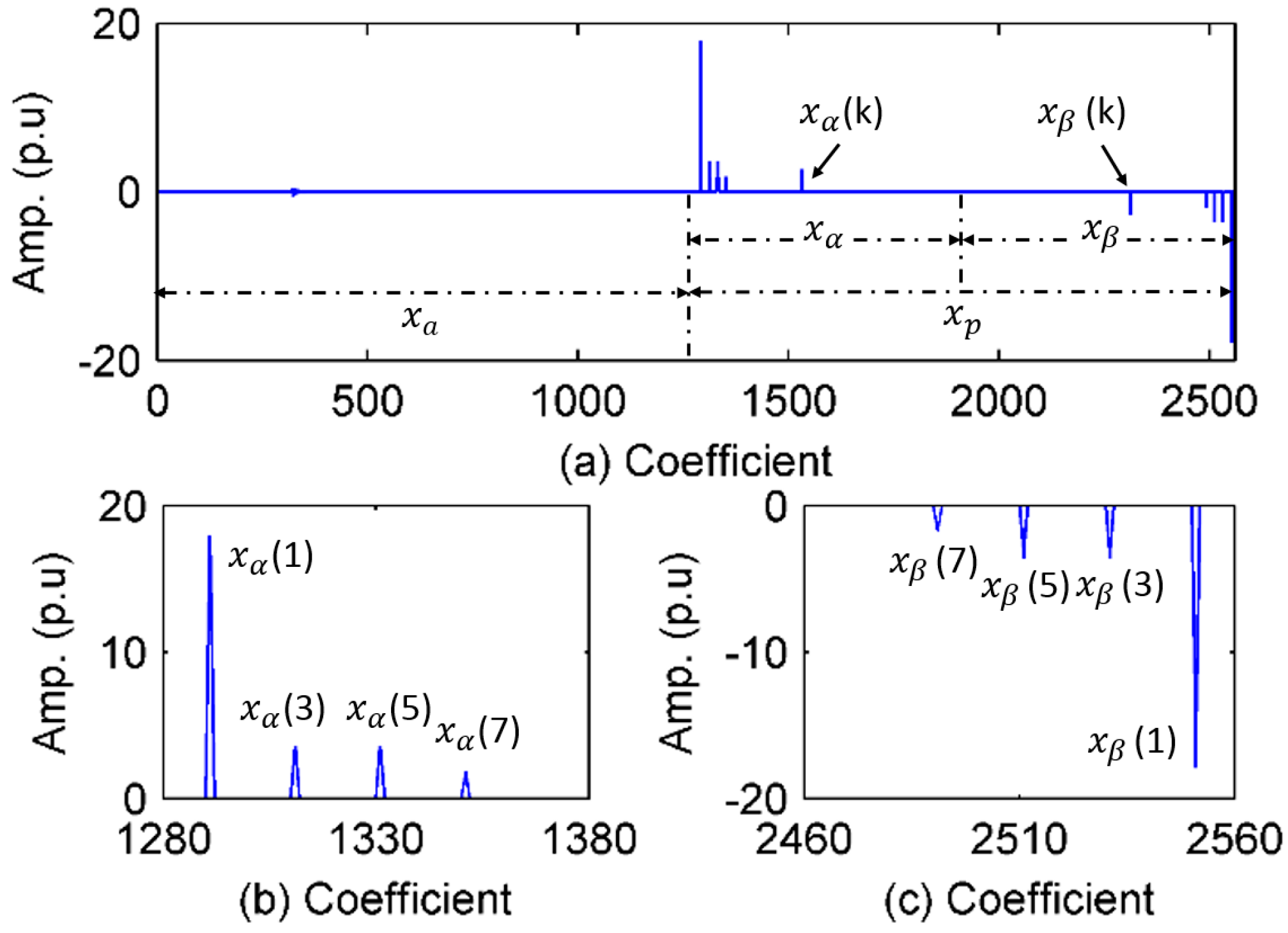
Suppose that
and
are extracted periodic and aperiodic components of signal
, respectively, and the
dictionary
, the Equation (1) can be rewritten as follows:
Therefore, it can be derived that
and
. According to the transform result of the Hartley transform, as shown in
Figure 1,
contains two
components,
and
, which are used for computing
and
where
,
, and
where
and
denote the MCs of the
kth harmonic in components
and
. The positions of
and
in
are center symmetric, as shown in
Figure 1b,c. Then, the amplitude
and the phase angle
of
th harmonic can be calculated as follows:
Regarding voltage sag, swell and interruption, they are often accompanied by oscillations at their start and end times. Hence, these components, like other existing transients, are mapped to the MCs corresponding to in the form of time-domain waveform. Owing to the fact that the sinusoidal components are mapped to the MCs corresponding to , the features of transients such as duration, start and end times , amplitude and polarity are obtained by presetting a threshold.
2.3. MPDs Recognition
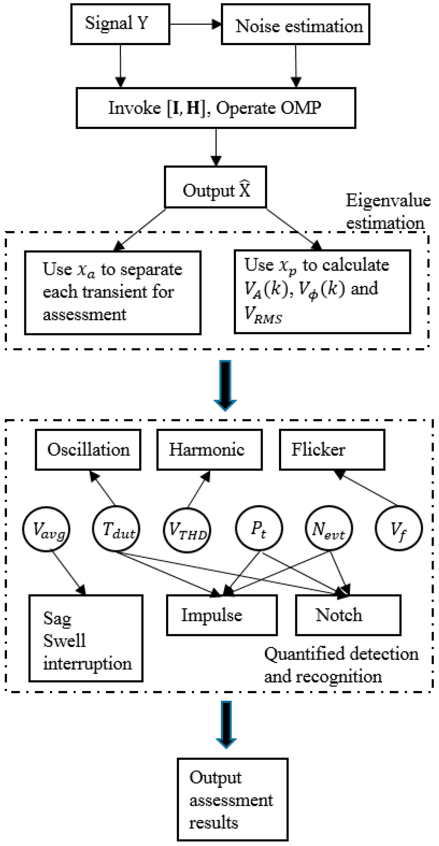
The outputs of joint-domain dictionary mapping contain the parameters of steady state components and separated transients. These quantities include amplitude, phase angle, frequency, duration time, and start and end times, which can clearly manifest the characteristics of each PD. Besides, all the extracted components of a signal can be separated from others, thus it can reduce the interaction effects and increase classification precision. On the other hand, when conducting MPDs, the appropriate features can lead to a more accurate classification result. The features for recognition in this paper are demonstrated in the following.
F1: Average value of biased root-mean-square (RMS) (). The process of detecting F1 is specified as follows:
- (1)
Recover the fundamental of a sampled signal using the equation below.
where
is the recovered fundamental waveform and
denotes the zeroized extension of “
” with its reserved position and value.
- (2)
Calculate the RMS of
, using the following equation:
where
is sample points per cycle,
is the interval of two adjacent sample points,
.
- (3)
Use the equation below to calculate
where
denotes the magnitude threshold and its value is
p.u,
denotes the amplitude RMS envelope of the affected waveform and its value is
.
is used to differentiate swell, sag and interruption.
F2: Event duration (
). According to Institute of Electrical and Electronics Engineers (IEEE) PQ standard 1159
TM-2009, the duration time of each transient event differs. For instance, the duration ranges of oscillation and impulse (same as multiple notch) are
and
, respectively [
27].
is the difference of start and end times
, and this paper employs a predefined magnitude threshold of 0.01 p.u to filtrate the useless MCs.
F3: THD for harmonic recognition (
). This paper introduces
(taking 50 harmonics into consideration, according to IEEE standard 519
TM-2014 [
28]), as show below, for measuring the magnitude of harmonic distortion.
where
represents the effective value of
th waveform. Based on IEC61000-2-4 and IEEE standard 1159
TM-2009, the minimum tolerance of THD in power grid is 5%, beyond which loads may be affected. Therefore, this paper adopts
as critical value to determine whether harmonics exist. Let it be noted that whether the detected
or not, the estimated parameters of the harmonics are provided for assessment.
F4: Polarity of the transient mean amplitude (). This quantity is used for distinguishing impulse (F4 > 0) and notch (F4 < 0). is calculated by multiplying the signs of MCs and the signal. For example, if the sign of MC is plus and the sign of signal is minus at the same time node, then the polarity is recorded as “minus”. According to IEEE standard 1159TM-2009, an impulse has a high overvoltage and a strong attenuation, thus there may exist MCs with minus polarity adjacent to those of the impulse. To eliminate this effect, the magnitude of the threshold is designated as 0.05 p.u. However, F4 is insufficient to differentiate an impulse from a notch.
F5: The number of detected transient events in same time interval (). Multiple notch, which is a periodic voltage disturbance, has constant event intervals other than impulses. However, repeated impulses with constant intervals may occur coincidently and affect the recognition of a notch. Hence, is used to differentiate individual types between repeated impulses (if F4 > 0, record F5 = 1; in other words, repeated impulses are recorded by repeated F5 = 1 rather than F5 > 1) and multiple notch (F5 > 1). F5 is computed by MCs corresponding to which have constant event intervals and minus polarity. The predefined magnitude threshold is 0.01 p.u. For every impulse or notch, it will generate a group of F2, F4 and F5 for precise recognition.
F6: Frequency value of the amplitude envelope of the affected waveform (). is obtained by using the index of minimum value of autocorrelation of with the sampling rate of the signal. The value is for identifying flickers ( 25 Hz).
Table 1 shows the classification rules of JDM by using the quantified eigenvalues. Due to the fact that these quantities have physical significance and directly reflect the level of each event, it enables the QEC to achieve a good recognition performance. On the other hand, the implementation strategy of recognizing MPDs is that JDM transforms MPDs into separated components and identifies them one by one. In other words, JDM is a component decomposition machine which converts a MPD issue to multiple SPD issues. In this way, the recognition precision of complex MPD is improved to a certain extent.
2.4. JDM Method for MPD Assessment
The proposed JDM method is focus on two tasks, including parameter estimation and MPD identification. For better understanding the work of this paper, the structure of JDM as a measurement of MPDs is shown in
Figure 2. In this paper, the OMP algorithm is adopted to achieve an optimal mapping solution. The OMP method has advantages in aspects of computational complexity and estimation accuracy [
29]. Moreover, JDM, which benefited from the OMP and the time-frequency dictionaries, leads to each components of a signal being precisely mapped to its optimal domain of
.
The detailed execution of the proposed JDM is structured as follows:
Step 1 Preprocessing of dictionary and noise level
- (1)
According to the sampling rate, use the Equation (8) to generate the basis and construct the joint dictionary .
- (2)
Use 4 level db4 wavelet to decompose signal .
- (3)
Estimate the noise level of input signal
using the formula proposed in [
30], as shown below.
where
denotes the noise variance and
is the first level of the wavelet transform.
Step 2 Calculation of MCs
- (1)
Input , and , then execute initialization: iteration time , index set , support set and residual . In the following process, , , and denote index, index set, support set and solution of iteration, respectively. denotes the th column of . and respectively denote the values of and when the iteration is terminated.
- (2)
Compute , then execute and .
- (3)
Calculate the least squares solution of : .
- (4)
Update residual .
- (5)
Judge termination condition ; if “yes”, terminate iteration. Then output the expanded form of by calculating and . If “no”, execute and jump to step 2).
Step 3 Estimation of eigenvalues
Calculate Equation (11) to obtain the amplitudes and the phase angles of each harmonic component. Use the extracted to compute the features of each transient as well as the start and end moments of sag, swell and interruption. The eigenvalue estimation is flexible and can be designed for the preferences of users.
Step 4 Recognition of PD
Estimate the necessary features for recognition according to the principle in
Table 1, then execute the QEC and output the result of identification.
can be constructed by using FFT and then doing linear transformation, thus the computational complexity (CC) is . The CC of OMP algorithm is where is the total iteration time, which changes with the complexity of signal components. When the components of a signal are added, also increases. However, because of the compactly supported characteristic of JDM, is still much less than . Therefore, the CC of the proposed JDM is which mainly comes from OMP.
3. Simulation Test
In this section, an example validation and classification experiment are presented for testing JDM. The MPDs, which are contaminated with Gaussian white noise, consist of the most popular SPDs in [
2,
5,
7,
8,
10,
11,
17,
19] in recent years. These studied SPDs include sag, swell, interruption, harmonic, flicker, oscillation, impulse and notch. The PDs are the sample rate of all test signals of ten cycles, which is 6.4 KHz, and the models of those SPDs are based on the IEEE PQ standard [
27] and previous works [
10,
17] as shown in
Table 2.
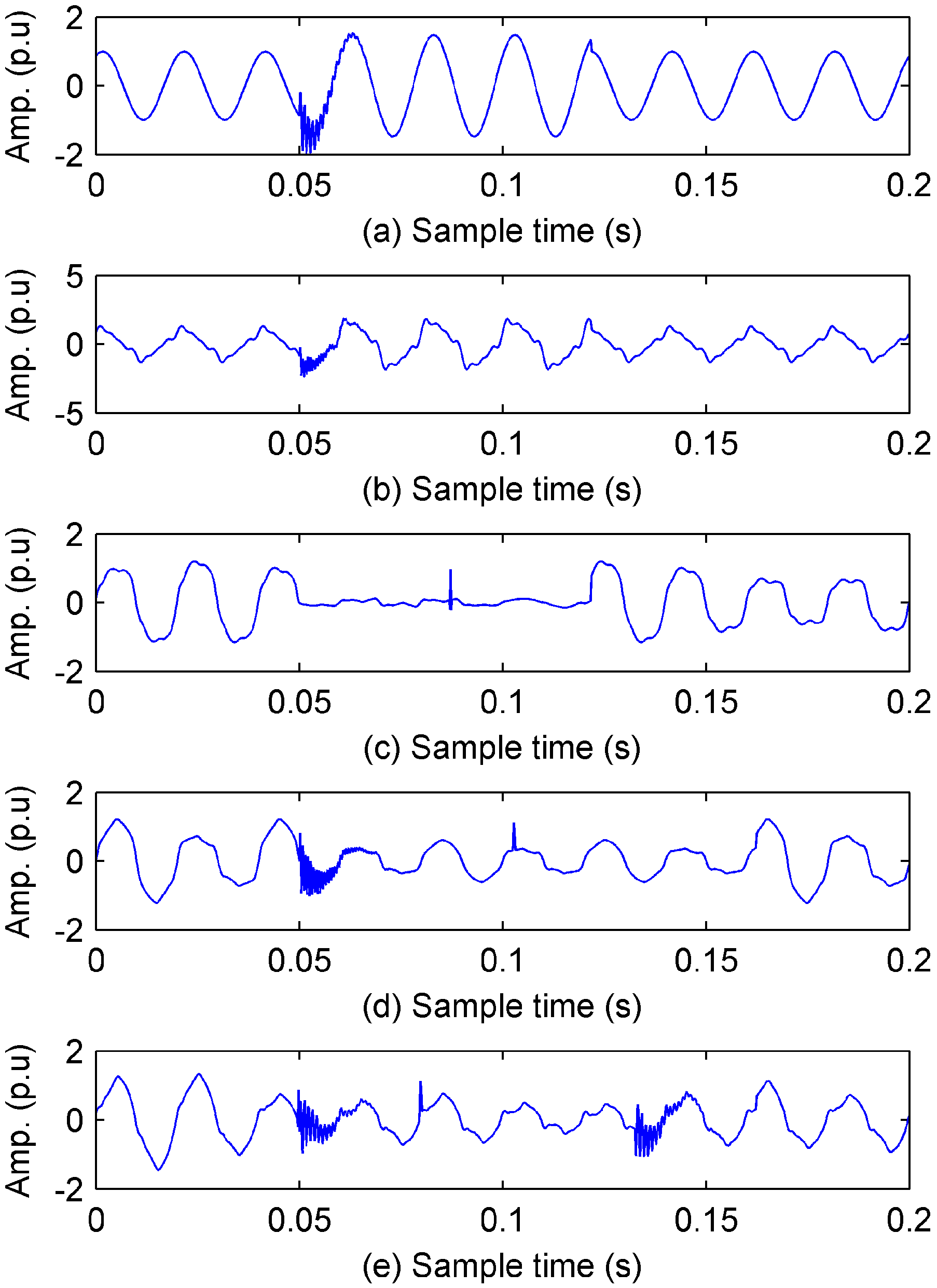
3.1. Example Validation
Without the loss of generality, a case containing sag, harmonic, flicker, two oscillations, impulse and noise was introduced to demonstrate the parameter assessment and the feature calculation of JDM. The details are shown in
Table 3.
Owing to the wide frequency spectrum of the transients, it is difficult to calculate the parameters of the MPD directly using FFT. In other words, the energies of each transient in the frequency domain was incompactly supported, especially for impulse. However, the JDM method takes advantages of the principle of compactly supported mapping in that it can separate out each component and execute each assessment independently. It can be seen from
Figure 3 that each transient was extracted, and the harmonics of each frequency and the RMS envelope were detected. The SSD technique [
20] can also separate the transient components, thus a comparison between JDM and SSD on parameter estimation is provided in
Table 4. To evaluate the level of estimation precisions, a mean error (ME) is introduced as follows:
where
denotes the error of the
th harmonic parameter and
is the total number of harmonics. As the fundamental value varies with the fundamental sag, the calculation of
is expressed as follows:
where
denotes the estimated amplitude of the
th
cycle of the
th
waveform. The
is calculated by JDM with
as input
and
.
For oscillation and impulse, the compactly supported MCs are generated on dictionary
, thus they contain their waveforms of the time domain which contribute to the calculation of
,
,
,
and
, as shown in
Figure 3a–c. Regarding harmonic components, MCs are compactly supported on the Hartley basis
, and the amplitude and phase of each harmonic, as well as
, can be directly computed by employing Equation (11). The calculated spectrum and phases of harmonics are shown in
Table 4 in detail.
Figure 3e presents the RMS envelope of the fundamental component which is used to obtain
and
. Therefore, JDM can efficiently transform the complicated MPD into a combination of SPDs which are easy to assess.
The quantified features of the JDM method for recognition is presented as follows:
p.u,
s,
s,
s,
,
,
Hz,
, as shown in
Figure 3f. Thus it can be concluded through the recognition rule of the QEC that the investigated signal contains sag, two short-term oscillations, impulse, harmonics and flicker.
The given duration time of two oscillation events is 0.005 s for testing whether JDM is effective. The differences between the given curves and the detected curves show that the transient components were precisely extracted. For iterative convergence when executing OMP, the transient was prevented from being mapped to the Hartley basis
, which will led to incompactly supported MCs. On the other hand, flicker and harmonics were accurately identified by judging the quantified eigenvalues
and
, and these quantities can be outputted as the results of the PD assessment. From
Figure 3a it can be seen that the harmonics produced a waveform similar to multiple notch, but the results reveal that there was no impact on JDM. Regarding voltage sag, the error of the estimated
is acceptable although
was affected by the flicker component. It is worth mentioning that the THD curve of JDM is calculated after eliminating the effects of transients, thus the error of THD is small according to the given value.
From the MEs, it can be seen that JDM was better than SSD for parameter estimation. That is because the discrete cosine basis (recorded as
) and the discrete sine basis (recorded as
) in [
20] have a high cross correlation, i.e.,
. It caused relatively diverging coefficients, which led to small coefficients being difficult to capture, thus the error was increased. Regarding JDM,
belonged to
in this case. Since harmonic components were only mapped to the MCs of
, and
is a linear transform of
, the results are compactly supported, and the performance of estimation precision was better than that of SSD.
In order to further validate the aforementioned causes, a comparative experiment with a group of 500 simulated MPDs containing four harmonics with one oscillation under 30 dB noise were designed. The signals complied with the models in
Table 2, and each parameter was randomly generated within its given range. In this case, the
was calculated using Equation (15).
Table 5 presents the MEs of JDM and SSD on the detection of the harmonic parameters. The results indicate that the comprehensive performance of JDM was still better than that of SSD for parameter estimation. Meanwhile, it verifies that the high correlation of
leads to inevitably additional errors. On the other hand, the comparison of
shows that the
of JDM was more precise than that of SSD. The
of FFT was 0.653, which reveals that the transient components had an impact on computing THD.
3.2. Comparative Experiment of Recognition Accuracy
To investigate the classification accuracy of PDs based on QEC, this paper adopts a comparative experiment with several outstanding approaches which can conduct MPDs. For this section, 8 SPDs from
Table 2 were selected as study objects, and they were divided into 5 groups: G1 (sag, swell and interruption), G2 (harmonic), G3 (flicker), G4 (oscillation), and G5 (impulse and notch). The combination principles of simulated MPDs are listed as follows:
2 simultaneous PDs: Randomly select two SPDs from G1 to G5, such as harmonics with voltage sag, harmonics with flicker, or swell with oscillation. See
Figure 4a.
3 simultaneous PDs: Randomly select three SPDs from G1 to G5, such as harmonics with voltage sag plus oscillation, harmonics with flicker plus swell and sag with two oscillations. See
Figure 4b.
4 simultaneous PDs: Randomly select four SPDs from G1 to G5, such as harmonics with voltage sag plus oscillation and impulse, harmonics with flicker plus swell and oscillation. See
Figure 4c.
5 simultaneous PDs: Randomly select five SPDs from G1 to G5 (harmonics, flicker and oscillation must exist, then choose two more from G1 and G5). See
Figure 4d.
6 simultaneous PDs: Randomly select six SPDs from G1 to G5 (G4 and impulse in G5 can be repeatedly selected) like the aforementioned MPD. See
Figure 4e.
In practice, the effects of multiple oscillations on power grids differ from that of a single oscillation. For example, the MPD caused by the re-striking phenomenon of switched capacitor banks contains two oscillations. Its probability of an accident is two times that of single oscillation. On the other hand, there may exist multiple impulses in arc voltage of power cables. The instantaneous overvoltage caused by these impulses would be different, as well as their damage to power cables. Therefore, multiple oscillations and multiple impulses are both treated as multiple PD events.
The comparative methods include ST and decision tree (DT) [
17], Adaptive Linear Network (ADALINE) and Feedforward Neural Network (FFNN) [
19], and SSD and Hybrid Decision Tree (HDT) [
20] which have been proposed in recent years. The design parameters of each SPD were randomly generated, i.e., parameters varied within the given ranges. The numbers of SPDs and MPDs for testing were 100 and 500, respectively.
Table 6 shows a comparison of classification accuracy between the proposed JDM method and several related methods. In this paper, clear PDs and PDs under 20 dB noise are investigated for studying the robustness of the method against noise. Work in [
17] did not provide an experiment with clear PDs, and work in [
20] only took 30 dB noise into consideration. Moreover, in [
13,
16], only MPDs with two simultaneous events were examined. The work in [
17] just examined voltage sag with harmonics and swell with harmonics. Regarding the ADALINE and FFNN algorithms in [
19], they can not only achieve a high recognition accuracy under 20 dB noise, but they can also conduct analysis on complicated MPDs with as many as six simultaneous events. Similarly, the proposed JDM can precisely recognize even complicated MPDs and have a good robustness against noise. Furthermore, benefitting from quantified eigenvalues, the proposed JDM improves the classification accuracy compared with other works.
Several conclusions can be drawn, as shown in the following.
The eigenvalues of the study case with 6 simultaneous events can be more precisely estimated by JDM compared to SSD, especially for harmonics. That is because the dictionary approximates to the optimal dictionary . The high cross correlation of and of SSD causes the non-uniqueness of its solution, which leads to a solution deviation in terms of true solution.
The joint-domain theory indicates that JDM can separately map transients and sinusoidal components to different domains which contributes to an accurate achievement of estimated parameters for MPD assessment.
After obtaining quantified eigenvalues, JDM can transform the complicated MPD into simple SPDs. The QEC can accurately identify the class of each SPD, then provide comprehensive classification results.
The comparative experiment of 500 simulated harmonics revealed that the of JDM is closest to the true THD, compared to SSD and FFT. When dealing with real harmonics with transients, JDM can obtain a more reliable THD value.
The average classification accuracy of SPDs and MPDs under 20 dB noise is 92.88, which is the highest among the methods for comparison. The experiment results demonstrate that JDM can maintain high detection and classification accuracy, even for analyzing the MPDs with six simultaneous events.
4. Actual Assessment
In a practical application, the actual PDs always appear in a form of multiple disturbances. In order to validate the efficiency of the proposed JDM method when conducting an actual PD event, this paper adopts a complicated MPD from the IEEE Power and Energy Society (PES) database [
31], as presented in
Figure 5a. In this section, sample rate is 6.4 KHz and the length of the arc signal is 6 cycles, according to the length of the provided signals in the IEEE PES database.
Figure 5 shows the parameter estimation of JDM for conducting an arc event. From
Figure 5b, it can be seen that the multiple transients had a constant interval of half-cycle, but the duration time of each was much less than 5 ms and the polarities were plus. Then, the transient eigenvalues were both recorded as all
, multiple
and all
s, thus the multiple transients were periodic impulses. Although there existed several minus polarity transients in the short-term, their intervals were varying, thus they were not recorded.
Figure 5c presents the RMS envelope of the extracted fundamental waveform. The estimated eigenvalues for identifying sag, swell, interruption and flicker were recorded as follows:
p.u and
Hz. Therefore, the whole signal was in a state of sag, and no flicker component was in the original signal. As the entire waveform was in sag, Equation (15) was used to compute
. The estimated THD
% reveals that the harmonic content of the arc voltage was far beyond what the grid can bear. In conclusion, the investigated MPD contained repeated impulses, voltage sag and harmonics.
Generally, an arc voltage, which is caused by a self-maintained discharge on a cable, contains periodic impulses at each initiating terminal of half-wave. Meanwhile, the magnitude of the arc voltage presents continuous sag and its waveform is severely distorted owing to high order odd harmonics [
16]. According to the records of the IEEE database, this MPD increases arc resistance as well as the temperature of cable, which leads to a permanent fault of the cable, i.e., a continuous arc. Therefore, the assessment of these complicated MPDs can avoid damage to power elements thereby reducing economic loss. Based upon the above analysis, it can be concluded that the recognition results of JDM agree with reference [
16]. From the actual experiment, several conclusions can be drawn:
In practice, the design of the joint-domain dictionary with low correlation is still effective, so that JDM can efficiently separate the transient components, and the impacts on the estimation of harmonics are considerably reduced. Therefore, it can achieve a good assessment performance even for real and complicated MPDs.
In the actual experiment, JDM has the ability to extract transient components, as can be seen by comparing the extracted repeated impulses in
Figure 5b with the original transient disturbances in
Figure 5a. Therefore, the
without the effects of the transients can be regarded as close to the real value.
The measurement and the classification mechanism of JDM are still effective for dealing with actual signals. In this case, JDM can still transform the complicated MPD into SPDs. The detection and recognition results, which agree with the comments of reference [
16], are authentic.
5. Conclusions
To achieve compactly supported mapping, this paper adopts a joint-domain dictionary with low cross correlation, and its approximate optimality has been verified. The effectiveness of the proposed JDM was tested by a study case of a MPD containing 6 simultaneous events and a group of MPDs. The estimation results of the simulation reveal that using the JDM method can efficiently separate the transient components, then it successfully transforms a MPD into some simple SPDs, thereby sensing the features of each event. JDM can achieve a more reliable THD than SSD and FFT. The MATLAB simulation test under noise conditions has been presented and the results revealed that JDM has a good robust performance against noise. Moreover, a comparative experiment with several related methods for validating the classification precision of JDM has been presented. The results indicate that the JDM method has a high recognition precision and a wide classification scope when dealing even with complicated MPDs.
In order to study the effect of JDM on practical problems, an actual arc voltage of a power cable, provided by the IEEE PES database was introduced. As transients and steady state components were successfully mapped to each compactly supported domain, JDM still precisely extracted each impulse component and a frequency spectrum which conformed to the actual features of the arc. Furthermore, a reliable classification conclusion was drawn according to the quantified eigenvalues, and it also agrees with the actual knowledge. Therefore, it can be concluded that JDM is a good method for assessing MPDs, including parameter estimation and recognition.


