Acoustic Wave-Based Method of Locating Tubing Leakage for Offshore Gas Wells

College of Mechanical and Transportation Engineering, China University of Petroleum-Beijing, Beijing 102249, China
*
Author to whom correspondence should be addressed.
Energies 2018, 11(12), 3454; https://doi.org/10.3390/en11123454
Submission received: 31 October 2018
/
Revised: 22 November 2018
/
Accepted: 6 December 2018
/
Published: 10 December 2018
Abstract
:This paper presents a novel acoustic wave-based method for the detection of leakage in downhole tubing of offshore gas wells. The localization model is developed on the basis of analyzing the propagation model of leakage acoustic waves and the critical factors in localization. The proposed method is validated using experimental laboratory investigations that are conducted to locate tubing leakage by setting five holes at different positions on the tubing wall. A detection system is developed for the leakage acoustic waves in the tubing-casing annulus, where one acoustic sensor is installed at the annulus top. Laboratory experimental results show that the depth of downhole leakage can be effectively located by using the proposed localization model. The localization errors are kept at a very low level, and are mainly generated from extracting the characteristic time and calculating annular acoustic velocity. A case study focusing on an offshore gas well is presented to illustrate the feasibility of the proposed method, and to demonstrate that the proposed model can locate the liquid level and leakage points under field conditions. The test can be performed without interrupting the production of gas wells.
1. Introduction
Downhole tubing is an important structure in a gas well and provides a flow path for natural gas in a reservoir. Downhole tubing is susceptible to leakage due to downhole operation, corrosion, and aging. Tubing leakage is a common issue, especially in offshore gas fields [1]. A case study of the Gulf of Mexico Outer Continental Shelf shows that such leaks will cause sustainable annulus pressure, interrupt the safe production of natural gas, and even result in blowout incidents [2,3]. Therefore, addressing downhole leakage is necessary to guarantee the safe operation of gas wells and further enhance the integrity management of offshore gas wells.
In general, downhole leaks are detected by measuring and analyzing the abnormal signals that are generated as leak flow moves through holes in the tubing, e.g., temperature, flow rate, and acoustic signals. Traditional logging methods, including flowmeter logging [4], temperature logging, ultrasonic logging [5], noise logging [6], and the integrated approach [7], can be used to measure abnormal signals by placing logging tools in the tubing. The abnormal signals in the tubing are measured and recorded by the sensors installed on the logging tools during lifting. The positions that correspond to the abnormal signals are considered as the depth of the leakage. However, the logging methods do not always produce the best results and might provide questionable results to operators. Recently, distributed sensor arrays (such as hydrophone, fiber-optic acoustic sensor, and fiber-optic temperature sensor) have been applied to measure these signals in onshore oil and gas wells [8,9,10]. Leakage is detected by performing beamforming and comprehensive analysis of the signals measured by each sensor. The instrument does not move in the tubing. The test precision is relatively improved by the distributed sensor array. However, the results greatly rely on the reliability of the instrument and the efficiency of signal processing. The current implementation of logging and distributed sensor arrays requires the instrument to be placed in the tubing, and the well needs to be shut down during testing. This process usually entails large costs and risk. Therefore, detecting tubing leakage without interrupting well production is necessary.
Tubing leakage will cause pressure changes in the tubing-casing annulus. Zhu et al. have introduced a calculation model of tubing leak depth based on the pressure balance principle when investigating the prediction model of annulus pressure in the CO2 injection well [11]. Wu et al. further studied this principle and extended it to production gas wells [12,13]. The Bayesian inference is introduced to handle the uncertainties in leakage location forecasting that are caused by variations in reservoir conditions and measurement errors. Meanwhile, an annulus pressure monitoring system is developed to assist diagnosis. This method is theoretically feasible, and does not affect the well production. However, the accuracy of results greatly relies on the wellbore fluid calculation and production status. The locating process needs the production and annulus pressure to be kept stable. This method also requires accurate liquid level information in the annulus, and is not suitable for a well that leaks at an excessive inclination or horizontal sections. Zhang et al. presented a method based on the application of a He tracer [14]. The tracers are injected from the annulus and detected at the choke. The leak depth is calculated by using the flowing time of the He tracer in the wellbore. This method is effective for judging the existence of leaks. The locating results are greatly affected by the calculation of wellbore pressure. This method is complicated to implement and not suitable for gas-lift wells. In addition, Ding et al. researched a method of detecting tubing leaks in horizontal sections of an intelligent well based on negative pressure waves [15]. In this method, the downhole pressure gauge needs to be permanently installed in the borehole. Taylor et al. also found leaks from echo curves in liquid level testing [16]. The above methods have been proposed in recent years and are in the theoretical research stage, lacking field applications and follow up reports due to limitations in their use. Therefore, investigating a detection and localization method that has a wide application range and convenient operation is significant.
The acoustic method is popular in detecting abnormal conditions in ground pipelines [17]. Three basic acoustic-based locating principles are used. The first principle uses the cross-correlation of two measured acoustic signals at both ends of the detection section [18]. Accuracy greatly relies on the time difference and wave velocity, and is improved by cross-correlation function models [19]. However, this method is not efficient if the acoustic sensor is located at the same side as the leakage. The second principle is based on the propagation properties of acoustic waves, and the distance between the leaks and sensor can be obtained by analyzing the amplitude change of the acoustic signals [20]. The attenuation coefficients need to be modified in every case [21], and the location accuracy is low. The last principle is based on the distributed acoustic sensor array. The location of the leaks can be found after beamforming and comprehensive analysis [22,23]. This principle is suitable for long-distance pipelines, where numerous sensors need to be set. More importantly, these methods require the simultaneous measurement of acoustic signals. These principles are difficult to implement in gas wells, because the acoustic sensors cannot be conveniently installed in the downhole, where the conditions are more complex. Therefore, developing a new acoustic-based locating principle suitable for downhole tubing leaks is essential.
This paper presents a ground method to detect and locate downhole tubing leaks in gas wells. Such a method requires one acoustic sensor to be installed in the annulus top. The localization model is derived by analyzing the localization principles, extracting the time difference, and calculating the acoustic velocity in the annulus. In addition, a double-layered experimental system is established to verify the theoretical model. A series of experiments under different leak positions are then designed and conducted. Finally, a field test is conducted, applying the proposed method. The testing process only needs to be performed at the top of the annulus, and will not interrupt gas production. The test process can be carried out at any time, and has a wide range of applications.
2. Theory and Methods
2.1. Principles
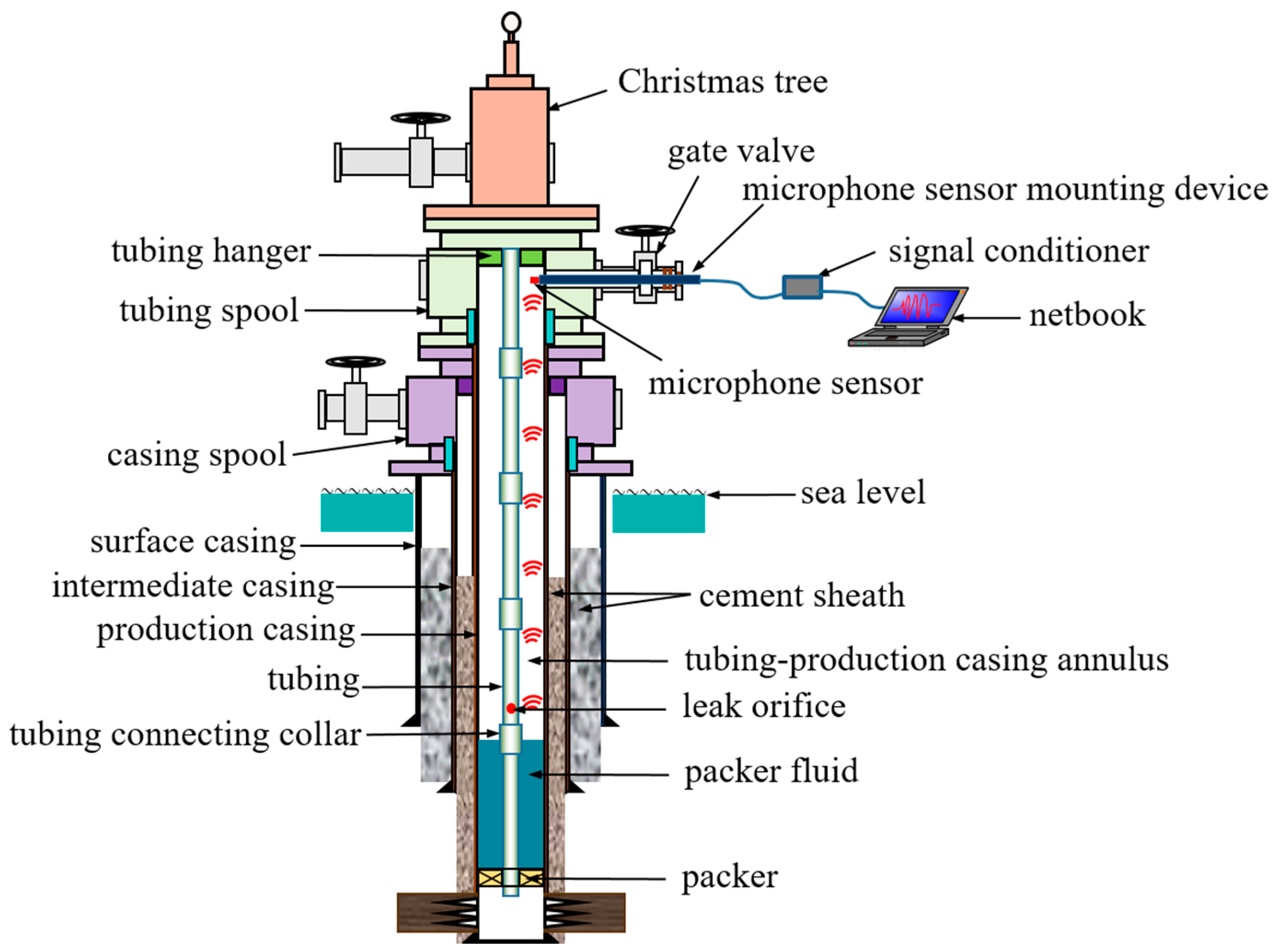
As shown in Figure 1, the wellbore consists of several concentric tubular columns. The annular space between the adjacent tube strings is known as the annulus. Under normal conditions, the natural gas in the reservoir completely flows to the wellhead through the tubing and then flows into the next pipeline through the Christmas tree. When tubing leaks, natural gas will leak into the tubing-casing annulus.
Acoustic waves will be generated by tubing leakage and then propagated in the wellbore. As shown, acoustic waves have four propagation paths, namely tubing fluids, tubing, annulus fluids, and production casing. The acoustic waves can be monitored by acoustic sensors installed in these media. However, the acoustic sensor cannot be easily installed in the tubing fluids during production. The cement sheath outside the production casing would affect the measurement of acoustic waves that propagate in the casing [25]. The vibration of the tubing causes difficulties in installing the sensor and measuring the acoustic waves. Installing the sensor in the annulus to monitor acoustic waves in the annulus is the best way to detect the leakage waves [26].
Figure 1 shows the schematic of the proposed method. With the use of a designed device, the microphone sensor is placed in the annulus. The leakage waves that propagate in the annulus are collected at the ground.
The tubing-production casing annulus is a closed space, both ends of which are sealed through the tubing spool and packer fluid. Two main reflecting discontinuities in the annulus are the liquid surface and tubing hanger. The leakage acoustic waves will travel upward and downward in the annulus simultaneously. The portion of the acoustic waves that travel to the annular top will be reflected by the tubing hanger and travel down to the liquid level. Similarly, the portion of the acoustic waves that travel to the annular liquid level will be reflected and travel to the top. These processes will continue until the acoustic energy is completely attenuated. As shown in Figure 2, three types of propagation modes of leakage acoustic waves in the annulus are analyzed. P1 is the portion of acoustic waves traveling downward and then upward. P2 is the portion of acoustic waves traveling upward. P3 represents the acoustic waves after multiple reflections. Therefore, the signals gathered by the microphone sensor simultaneously contain P1, P2, and P3. A time delay exists when P1, P2, and P3 propagate to the microphone sensor, which can be obtained through proper signal processing. The process will be described later.
The following expressions show the relationship between the distances in Figure 2:
where is the average acoustic velocity in the annulus (m/s); t1 is the time delay between P1 and P2, which is equal to the travel time of the acoustic waves from the leak depth to the liquid level then back to the leak depth (s); t2 is the time delay in P3, which is equal to the travel time of the acoustic waves from the tubing hanger to the liquid level then back to the tubing hanger (s); L is the liquid level in annulus (m); and x is the leak depth (m).
The leak depth can be expressed by
Therefore, the critical factors for the accurate localization of tubing leakage using this method are the characteristic time (t1 and t2) and acoustic velocity in the annulus.
2.2. Acoustic Velocity in the Annulus
American Gas Association (AGA) Report 10 gives the acoustic velocity of natural gas [27], which is mainly affected by the composition, temperature, and pressure of the gas.
where k is the ratio of specific heats (dimensionless), R is the mole gas constant (J/(mol·K)), Mg is the molar mass of natural gas (kg/mol), T is the gas temperature (K), Zg is the compressibility factor of natural gas (dimensionless), and ρ is the gas molar density (mol/m3).
The molar density and compressibility factor are calculated by the empirical equations proposed by Coquelet [28], which utilize the PR equation of state. Before calculating the acoustic velocity in the annulus, the annular temperature and pressure need to be determined.
2.2.1. Temperature Distribution in Annulus
Heat transfer occurs between the production fluids and the surrounding media in a flowing well due to the temperature difference. The temperature distribution in the wellbore can be derived on the basis of the fluid–energy balance and heat transfer equations. It is assumed that [29,30] (1) the heat transfer in the wellbore is in a steady state, while the heat transfer from wellbore to the formation is in a non-steady state; (2) only radial heat transfer is considered; and (3) the formation temperature varies proportionally with depth. Therefore, the equilibrium equation for the element dH, which is shown in Figure 3, can be expressed as
where Tf is the tubing fluid temperature (K), H is the measured well depth (m), cpm is the heat capacity of the tubing fluid at constant pressure (J/(mol·K)), Q is the heat flow rate (J/s), wt is the mass flow rate (kg/s), g is the gravitational constant (m/s2), θ is the angle of inclination (degrees), u is the gas velocity (m/s), CJ is the Joule–Thomson coefficient (K/Pa), and pf is the pressure in the tubing (Pa).
On the basis of the principles of heat transfer, the heat transfers from tubing fluids to the cement–formation interface, and from this interface to formation can be described by
where U is the overall heat transfer coefficient, which is related to the heat resistance from the structures between the tubing fluids and the formation [32,33] (W/(m2·K)); rti is the inner radius of the tubing (m); Ke is the thermal conductivity of the formation (W/(m·K)); D(t) is the dimensionless temperature function [34]; Tcfi is the temperature at the interface (K); and Te is the formation temperature (K).
Combining Equations (4) and (5), the following differential equation can be obtained:
where and , which can be calculated by an empirical formula [31].
Then, the iterative formula for the temperature of tubing fluids can be derived by solving Equation (6).
Similarly, the heat transfer from outside of the tubing to the cement–formation interface, and from the inside of the casing to this interface, can be expressed as
where U1 is the heat transfer coefficient between the outer tubing surface and the cement–formation interface (W/(m2·K)), U2 is the heat transfer coefficient between the inner casing surface and the cement–formation interface (W/(m2·K)), rto is the outer radius of the tubing (m), rci is the inner radius of the casing (m), Tto is the temperature at the outer tubing surface (K), and Tci is the temperature at the inner casing surface (K).
Combining Equations (5) and (8) obtains the expression of annular temperature
2.2.2. Pressure Distribution in the Annulus
The annulus pressure can be calculated by using the integration method [24], which can be expressed as
where pa is the annulus pressure (Pa) and ρg is the natural gas density (kg/m3).
The annular gas density can be derived from the gas state equation
Substituting Equation (11) into Equation (10) and making an integral, the annulus pressure in element dH can be obtained.
where pai represents the outlet pressure of segment i, which is equal to the inlet pressure of segment i + 1.
As shown in Figure 3b, the wellbore is first divided into N segments from the wellhead to the bottom-hole. The parameters of every segment can be obtained by successive iterations using Equations (9) and (12). After obtaining the annular temperature and pressure, the acoustic velocity in the annulus can be calculated.
2.3. Extraction of Characteristic Time
Original signals usually contain noise. This noise affects the accuracy of characteristic time extraction and must be eliminated. In this paper, the wavelet threshold de-noising method is used to filter noise in original signals. With the use of wavelet decomposition, wavelet coefficients correction, and wavelet reconstruction, the noise can be largely eliminated [35]. When performing wavelet decomposition, the db10 wavelet is used as the wavelet basis, and the decomposition level is five.
The autocorrelation function can reflect the correlation of two values of a random signal at the time interval τ [36], which is defined by
where τ is the time delay.
In practice, can only be estimated, and the basic estimator is given by
where Tim is the time window.
Generally, the autocorrelation function is expressed in a normalized form [37]. It is defined as
which means that ρss(τ) will reach the peak value if s(t) and s(t + τ) are correlated. Theoretically, the leakage acoustic signals generated at the same position and time are strongly correlated, whereas those generated at different positions or different times lack correlation. Therefore, the characteristic time can be obtained through autocorrelation analysis of de-noised signals.
According to the location principles, when , will reach a negative extreme value. When , will reach a positive extreme value. Similarly, when (n = 2, 3, 4 …), will reach positive extreme values as well.
Next, t1 and t2 are obtained by extracting the extreme values of . Figure 4 shows the autocorrelation curve of the acoustic signals collected in tubing leakage. The method of extracting the characteristic time is presented, with t1 corresponding to the first negative peak and t2 corresponding to the first positive peak in the autocorrelation curve.
2.4. Model for Locating Downhole Tubing Leakage
As analyzed in Section 2.2, the temperature and pressure in the testing annulus can be expressed as a function of depth and time. Generally, the acoustic waves reach the wellhead in seconds. During this time, the state parameters of the annular gas do not change. Therefore, the acoustic velocity in the annulus can be expressed as a single-valued function of depth.
Equation (1) can be rewritten as
The liquid level L and leakage depth x can be obtained by solving Equation (16). The following functions are established.
Then, the problem is transformed into solving and , which can be achieved by using the dichotomy searching method [38].
In summary, as shown in Figure 5, the locating procedures are divided into three steps:
Step 1: Acoustic velocity and characteristic time are calculated. First, the temperature and pressure distributions in the annulus are obtained based on wellhead temperature, pressure, and the specific gravity of production gas, using Equations (9) and (12). The acoustic velocity distribution in the annulus is calculated using Equation (3). Then, noise reduction and autocorrelation analysis are performed on the measured acoustic signals. The characteristic times t1 and t2 are extracted from the autocorrelation curves according to the method proposed in Section 2.3.
Step 2: The liquid level is calculated. The liquid level is acquired by solving the first function in Equation (17), with the use of the dichotomy searching method. The value Lmid is equal to (L1 + L2)/2 in each iterative step.
Step 3: Leak depth is calculated. The leak depth is obtained by solving the second function in Equation (17), with the use of the dichotomy searching method. The value xmid is equal to (x1 + x2)/2.
3. Laboratory Experiments
3.1. Experimental System
To study the effectiveness of the proposed method, a series of laboratory experiments were designed and conducted with the experimental system, as shown in Figure 6 and Figure 7. The system contained a 47 m long tube string, tubing spool, gate valve, a set of compressors, high-pressure and low-pressure buffer tanks, many valves, and an acoustic data acquisition system. The tube string was a double-layered structure. Tubing with an outer diameter of 88.9 mm and casing with an outer diameter of 244.5 mm were used to simulate the wellbore structure, to which a full-scale tubing spool was connected at one end and sealed on the other. To simulate the liquid level in the annulus, a bent tube filled with water was added to the end of the tube string. A completely sealed annulus with a length of 46.9 m was formed. The experimental platform was horizontally placed, and the distance between the tubing spool and leak points on the tubing was the simulated depth of the leak location.
Compressed nitrogen was used as the gas source in the experiments, which was generated by a nitrogen generator and stored in low-pressure buffer tanks. Before the experiments, the gas was compressed and injected into high-pressure buffer tanks. From the high-pressure buffer tanks, the gas entered the tubing strings, flowed into the terminal buffer tank, and was finally discharged into the environment.
The data acquisition system contained an acoustic sensor, a signal conditioner, a data acquisition unit, and a computer. A CHZ401 pre-polarized condenser microphone with YG-401 preamplifier was chosen, with a sensitivity of 2.85 mV/Pa. The lower frequency response of the microphone was 1 Hz and the lower detection limit was 36 dB. The signal conditioner was a PM20B, which was manufactured by Beijing Acoustic Technology Company (Beijing, China), who also manufactured the microphone. A MCC E-1608 DAQ device was used to collect data. As shown in Figure 7, the acoustic sensor was installed in the annulus top using a designed device.
In addition, a Rosemount 644H temperature transmitter and 3051T pressure transmitter were used to monitor the corresponding parameters in the annulus and the tubing.
3.2. Experimental Design
As shown in Figure 8, five leak positions were set on the tubing string and were labeled a, b, c, d, and e. The distances between the acoustic sensor and the five positions were 45.75, 42.18, 39.18, 35.84, and 32.84 m, respectively. Only one hole leaked in each experiment. When the gas flowed through the tubing, some nitrogen would leak into the annulus, and acoustic waves would be generated and measured.
Table 1 shows the experimental design, in which the controlled variables are leak depth, orifice diameter, and differential pressure. The differential pressure refers to the difference between the tubing pressure and the casing pressure.
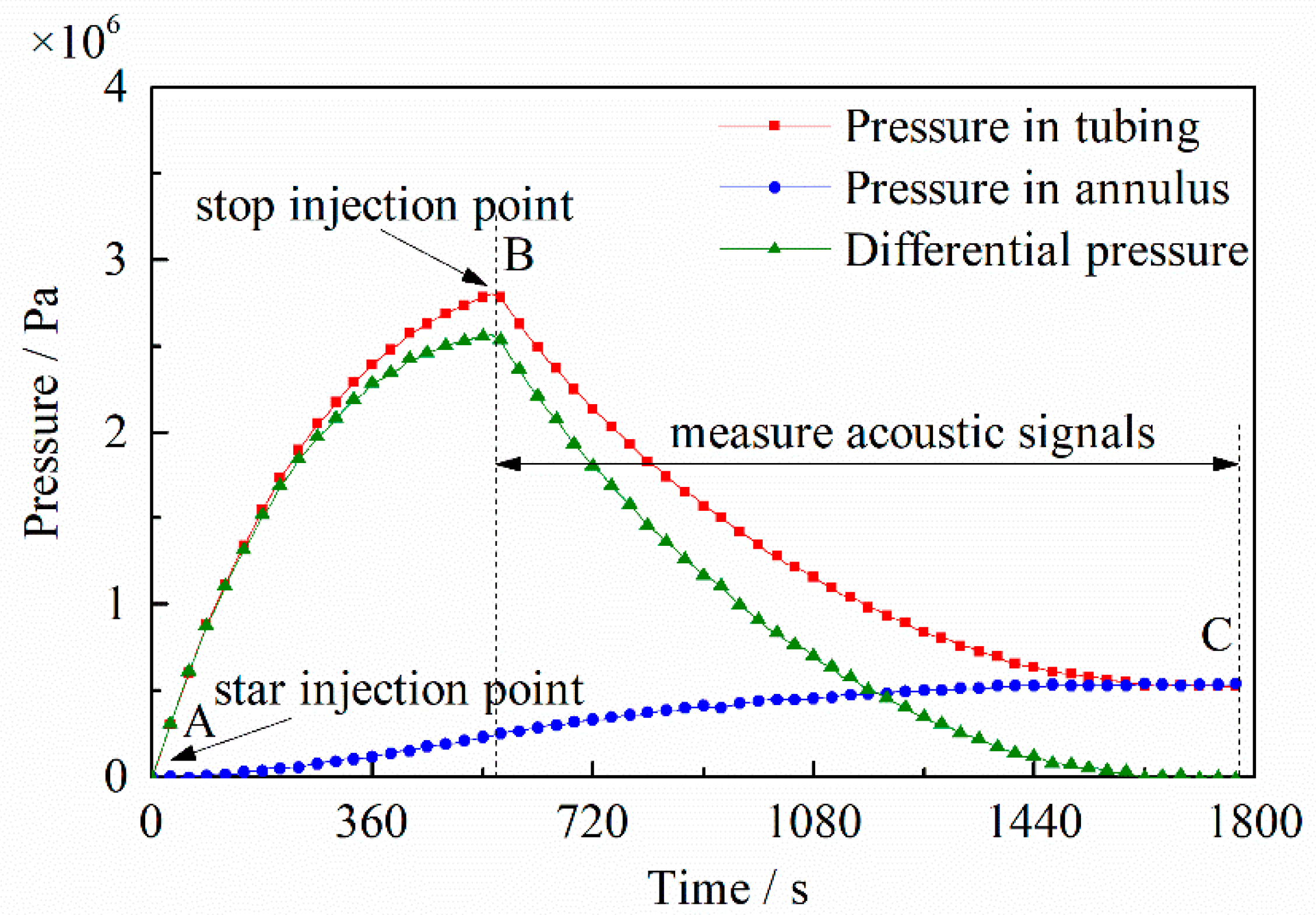
During experiments, the gas supply was stopped when the differential pressure reached a certain level, as shown in Figure 9. The acoustic signals were measured when the differential pressure in the BC segment reached the preset values. The sampling frequency of the acoustic signals was 30,000 Hz, and the sampling frequency of the pressure and temperature signals was 10 Hz. The measurements were repeated several times to ensure reproducibility.
3.3. Experimental Results and Discussion
The acoustic signals collected at the annulus top were analyzed before making localization analysis. Figure 10 shows the time and frequency domain distributions of acoustic signals collected at leak position a, at a differential pressure of 2.0 MPa and orifice diameter of 1.5 mm. The leak acoustic signals are random signals with a broadband frequency. The collected acoustic signals are mainly distributed in multiple frequency bands of 0–2500 Hz, and the energies are mainly distributed in the range of 0–130 Hz.
3.3.1. Leak Localization for Different Positions
First, the acoustic velocity in the annulus was calculated based on Equation (3). As shown in Figure 11, the acoustic velocities in the experimental annulus are approximately 357 m s−1 to 359 m s−1.
Then, the characteristic time was extracted, as shown in Figure 12a–e. After repeated verification, the optimal time window in the autocorrelation analysis was set as 0.4 s. A threshold for autocorrelation coefficients was set when extracting t1 and t2. The threshold was ±0.3. The characteristic time t1 varies with the leak positions, while t2 has the same value. This is due to the fact that t1 characterizes the distance between the leak point and liquid level, while t2 characterizes the length of the annulus (i.e., liquid level).
Figure 13 shows the theoretically predicted and extraction values of t1 and t2. The predicted values were calculated on the basis of Equation (16). When the leak point approaches the wellhead, the characteristic time t1 becomes larger. Conversely, the characteristic time t1 approaches zero. When t1 is small enough, the liquid level can be considered as the leak depth. As shown, the errors of extracting t1 are −2.44% to −0.20%, and the errors of extracting t2 are −1.14% to −0.37%.
Table 2 shows the localization results, in which the relative error is equal to the ratio between the distance difference and the actual length of the annulus. The distance difference is equal to the calculated distance minus the actual value. As shown, the leak points are effectively located. The absolute location error is on the order of cm. The relative errors generated in calculating the annulus length are −1.14% to −0.37%, and the relative errors for locating leaks are −0.97% to −0.33%. The errors generated in calculating annulus length are equal to the errors of extracting t2. The negative sign means that the calculated distances are smaller than the actual distances.
3.3.2. Leak Localization for Different Differential Pressures
The autocorrelation coefficients of the acoustic signals generated at different differential pressures are shown in Figure 14a–f. The theoretically predicted and extraction values for t1 and t2 are shown in Figure 15. The predicted values of t1 and t2 increase with differential pressure, because the large differential pressure corresponds to a small annulus pressure. This will result in a large propagation velocity and short propagation time for the leakage acoustic waves. The errors of extracting t1 are −1.94% to −0.81%, and the errors of extracting t2 are −1.07% to −0.82%. Moreover, the curves still have slight fluctuations even if the measured signals are subjected to noise reduction. The fluctuations are relatively obvious, especially when the differential pressure decreases. Thus, to extract the characteristic time more easily, the differential pressure should be increased as much as possible. In field testing, this can be actualized by bleeding the annulus pressure.
The localization results for different differential pressures are shown in Table 2. The absolute location error is on the order of cm. The relative errors generated in calculating annulus length are −1.07% to −0.82%, and the relative errors for locating leaks are −0.92% to −0.55%.
3.3.3. Leak Localization for Different Orifice Diameters
Figure 16 shows the autocorrelation curves of the measured signals for different orifice diameters. Figure 17 shows the corresponding characteristic time. Theoretically, t1 and t2 should be consistent for different orifice diameters, because the propagation of leakage acoustic waves is not affected by the leak size. Nevertheless, slight differences exist among the predicated values due to the difference in annular pressure and temperature in each experiment. The feature points are apparent and easily determined, even under the orifice diameter of 0.5 mm. In other words, a small leakage can be identified. From Figure 16, the errors of extracting t1 are 0.64% to 2.32%, and the errors of t2 are −1.59% to −0.45%.
The localization results for different orifice diameters are also shown in Table 2. The absolute location error is on the order of cm. The relative errors generated in calculating the annulus length are −1.59% to −0.45%, and the relative errors for locating leaks are −1.97% to −0.56%. For the leak hole of 0.5 mm, the locating accuracy is still high.
The errors generated in locating leaks results from the distance measurement and distance calculation. The reasons mainly come from the following aspects:
1. Errors in measuring actual distance.
The errors are caused by the system design and distance measurement, which occur in the laboratory experiments only. This type of error can be greatly reduced by repeating measurements.
2. Errors in calculating distance.
• Extraction of the characteristic time.
This type of error comes from signal measurement, signal processing, and characteristic time extraction.
Errors in measuring acoustic signals are caused by internal and external factors. The internal factors come from the signal acquisition system, which affects the comprehensiveness and authenticity of the measured signals. The external factors include environmental noise, airflow noise, and facility operation noise. This noise mixes with the useful signals and is difficult to eliminate completely.
Wavelet threshold denoising and autocorrelation analysis are the primary error sources in signal processing. The wavelet scale and the threshold decide the frequency band and amplitude of the signals used for autocorrelation analysis. A large scale will make the signals smooth but have less information. Generally, the scale should be set to make the frequency band of de-noised signals locate in the 1–130 Hz range.
Errors generated in extracting t1 and t2 come from the interference of abnormal fluctuations on the autocorrelation curves. These fluctuations are caused by the echoes of the collars and obstacles in the annulus and some periodic interference signals. The fluctuations affect the precise extraction of t1 and t2.
• Calculation of the acoustic velocity in the annulus.
The acoustic velocity increases with temperature and pressure. The accuracy of measuring annular temperature and pressure affects the calculation of acoustic velocity, and further affects the localization. The experimental nitrogen had a purity of 99.9%, which is considered as pure nitrogen during calculations. This approximate approach will produce errors as well.
Although the errors of each factor are difficult to quantify, the total errors are known. As mentioned above, the errors of t1 and t2 can be quantified. The errors of t2 are equal to the errors in calculating the annulus length. This shows that the errors of t1 and t2 are actually the combination of errors in calculating acoustic velocity and extracting characteristic time, and the errors in the process of locating leakages are smaller than the errors of t1. The total error is reduced during the localization process. Consequently, the process of extracting characteristic time and calculating acoustic velocity are the main error sources for this method.
To reduce the errors, relevant measures should be taken. First, the signal acquisition system and denoising method should be improved. Appropriate sampling frequency and time windows must be set to acquire more comprehensive leakage signals and characteristic time. Then, the temperature, pressure, and composition of annulus gas must be accurately measured or calculated.
Despite the above errors, this method is proven to be applicable in effectively locating leaks in downhole tubing.
4. Field Application
4.1. Description of Field Test
To verify the applicability of the proposed method in the field, an offshore gas well with serious tubing-casing annulus pressure was selected as a case study for analysis. The bleeding-off and build-up history of the annulus pressure shows that the annulus pressure is caused by downhole leakage. The pressure at the annulus top is almost equal to the pressure at the wellhead. The parameters of the gas well are shown in Table 3.
A test system was designed as shown in Figure 18. The type and installation of the acoustic sensor was the same as the laboratory experiments. As shown in Figure 18a, the flange was first connected to the gate valve, and the gate valve was opened slowly. Then the sensor was pushed into the annulus along the flow passage by rotating the driving gear. To adapt the field conditions, the signal conditioner, data acquisition unit, and power supply were integrated in an explosion-proof box.
Before testing, the annulus pressure needs to be relieved to form a large differential pressure between the tubing and the annulus. The sample frequency was set as 30,000 Hz. The temperature and pressure at the annulus top were measured during testing, as listed in Table 3.
4.2. Field Results and Discussion
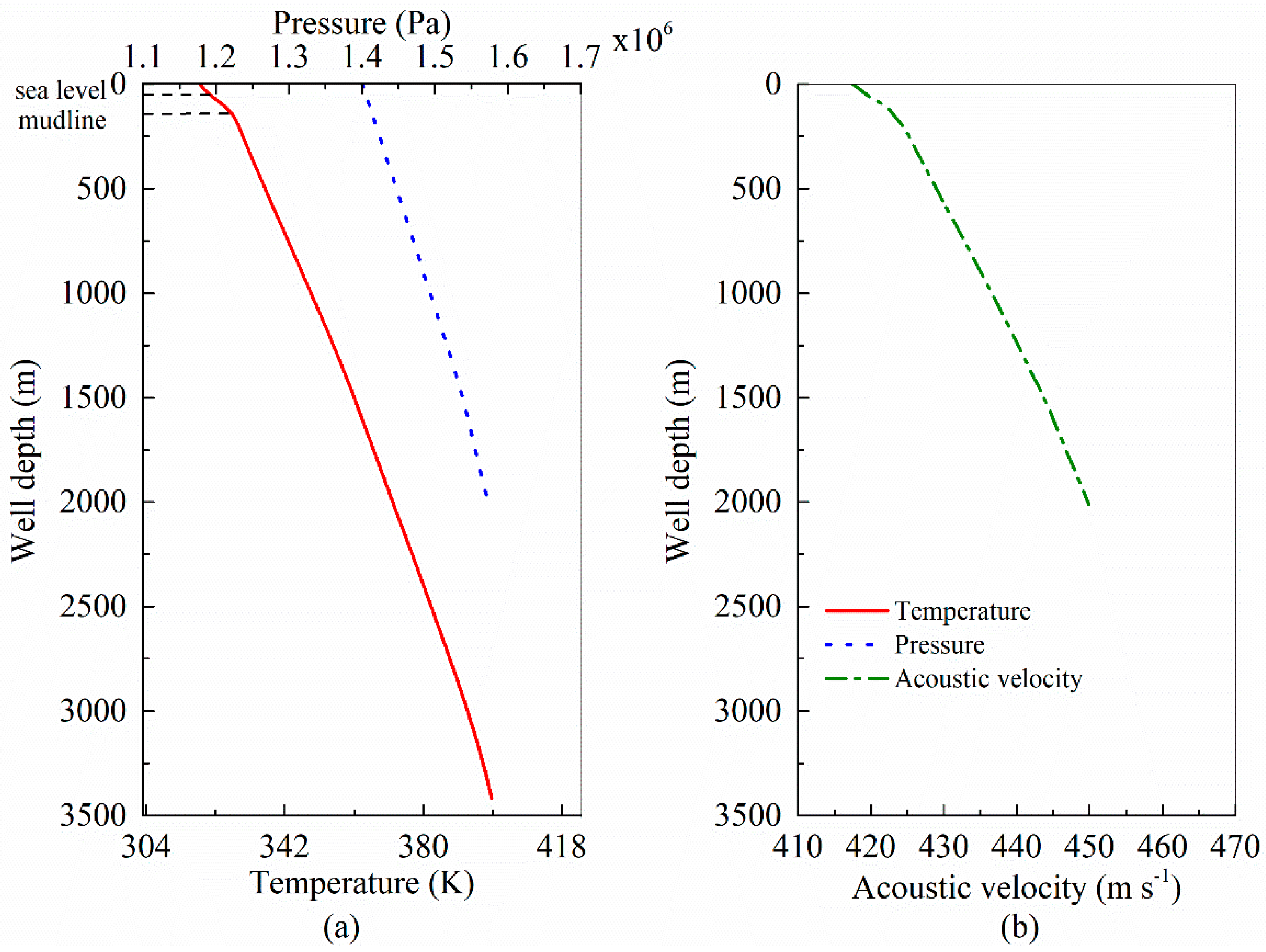
First, the acoustic velocity distribution along the annulus was calculated on the basis of the method mentioned in Section 2.2, as shown in Figure 19. The acoustic velocity varied from 415 m/s to 455 m/s and increased with depth.
Then, the characteristic time was extracted, as shown in Figure 20. The curve has the same distribution features as the laboratory experiments, but with more interference. This interference is mainly caused by the echoes of collars, the subsurface safety valve, and other obstacles in the annulus. The threshold for the autocorrelation coefficient was set to ±0.3. The extraction results are shown in Table 4. Notably, a significant positive peak S also exists on the curve. A comparison with the downhole string information shows that the S peak is caused by the echo of the subsurface safety valve.
Finally, the liquid level and the depth of S were calculated in step 2, as mentioned in the Section 2.4, and the leakage depth was calculated in step 3. As shown in Table 4, the testing well has leak points at depths of 1799.80 m. The liquid level in the tubing-production casing annulus is 2207.98 m. No excess structures exist, except for the tubing string around the leakage depth, as indicated by a comparison of the well completion information. The calculation depth of S is 240.57 m, which agrees with the depth of the subsurface safety valve at 238.23 m. The relative error is 0.98%. As shown in Table 5, the determined measurement errors in the laboratory and the field are compared. Despite the difference in test conditions between the laboratory and the field, the relative errors are close to each other, all within 1%. This further illustrates the accuracy of the proposed method. The result also shows that the obstacle will have no effect on the localization method, as long as the leak acoustic waves can propagate to the annulus top.
During the field test, the gas well was in production, and tubing leaks could be detected and located without interrupting the production of the gas well. The test only requires the acoustic sensor to be set in the annulus, which is simple and riskless, and the accuracy is satisfactory.
5. Conclusions
A novel method for locating downhole tubing leakage was developed in this study. The accuracy of the model in locating leakage points is validated through a series of laboratory experiments and field application. The following important conclusions can be drawn:
- The leakage acoustic waves of downhole tubing can be measured by an installed acoustic sensor in the annulus top, and the downhole leakage can be detected at the ground.
- The position of tubing leakage is located by autocorrelation analysis of the acoustic signals in the annulus. The localization model is developed. The fundamental steps and equations for this method are concluded.
- Though errors exist, the proposed model is able to locate the tubing leakage effectively. In the laboratory experiments, leaks as small as 0.5 mm in diameter could be located. The errors generated in the localization process were kept at very low levels. The absolute localization errors were on the order of cm, and the relative errors were within 1%. The errors are mainly determined by characteristic time and annular acoustic velocity.
- Field application demonstrated that the proposed method performs well in locating the depth of downhole leakage and the liquid level in the annulus. Therefore, the merits of the methods are concluded.
The acoustic wave-based method presents a novel method to deal with the issue of tubing leakage in gas wells. It provides guidance in annulus pressure management and downhole repair, as well as integrity management in production wells. In the near future, this improved method can be used for better long-term monitoring in the production field.
Author Contributions
Each of the authors contributed to performing the experiments and writing the article. D.L. is the main author of this manuscript, and this work was conducted under the advisement of J.F. S.W. reviewed the manuscript and made contributions to its structure.
Funding
This research was funded by the National Key Research and Development Program of China, grant number 2017YFC0804500.
Acknowledgments
The author would like to acknowledge the workers in the RongSheng Machinery Manufacture Ltd. Huabei Oilfield, Hebei for providing support in building the experimental platform. Special thanks are due to the anonymous reviewers for their useful comments and suggestions regarding the present paper.
Conflicts of Interest
The authors declare no conflict of interest.
References
- Degeare, J. Repaire of Csing Failures and Leaks. In The Guide to Oilwell Fishing Operations, 2nd ed.; Gulf Professional Publishing: Oxford, UK, 2015; Chapter 18; pp. 133–140. ISBN 978-0-12-420004-3. [Google Scholar]
- Bourgoyne, A.T.; Scott, S.L.; Regg, J.B. Sustained casing pressure in offshore producing wells. In Proceedings of the Offshore Technology Conference, Houston, TX, USA, 3–6 May 1999; p. 11029. [Google Scholar]
- Chen, P.; Gao, D.; Wang, Z.; Huang, W. Study on aggressively working casing string in extended-reach well. J. Pet. Sci. Eng. 2017, 157, 604–616. [Google Scholar] [CrossRef]
- Bennett, R.; Paul, D.S., Jr.; Gustafson, T.D.; Gillette, I.E. Measuring low flows in devonian shale gas wells with a tracer-gas flowmeter. SPE Form. Eval. 1991, 6, 269–272. [Google Scholar] [CrossRef]
- Johns, J.E.; Blount, C.G.; Dethlefs, J.C.; Loveland, M.J.; Mcconnell, M.L.; Schwartz, G.L.; Julian, J.Y. Applied ultrasonic technology in wellbore-leak detection and case histories in Alaska north slope wells. SPE Prod. Oper. 2009, 24, 225–232. [Google Scholar] [CrossRef]
- Michel, C.M. Methods of detecting and locating tubing and packer leaks in the western operating area of the prudhoe bay field. SPE Prod. Facil. 1995, 10, 124–128. [Google Scholar] [CrossRef]
- Al-Hussain, A.M.; Hossain, M.E.; Abdulraheem, A.; Gajbhiye, R. An integrated approach for downhole leak detection. In Proceedings of the SPE Saudi Arabia Section Annual Technical Symposium and Exhibition, AI-Khobar, Saudi Arabia, 21–23 April 2015; p. 77996. [Google Scholar]
- Bateman, R.M. Well and Field Monitoring. In Cased-Hole Log Analysis and Reservoir Performance Monitoring, 2nd ed.; Springer: New York, NY, USA, 2015; Chapter 14; pp. 244–260. ISBN 978-1-4939-2068-6. [Google Scholar]
- Hill, F.; Bond, A.; Biery, M.; Jagannathan, S.; Walters, D.; Lu, Y. Methodology and array technology for finding and describing leaks in a well. In Proceedings of the SPE Annual Technical Conference and Exhibition, Dubai, UAE, 26–28 September 2016; p. 181497. [Google Scholar]
- Julian, J.Y.; King, G.E.; Cismoski, D.A.; Younger, R.O.; Brown, D.L.; Brown, G.A.; Richards, K.M.; Meyer, C.A.; Sierra, J.R.; Leckband, W.T.; et al. Downhole leak determination using fiber-optic distributed-temperature surveys at Prudhoe Bay, Alaska. In Proceedings of the SPE Annual Technical Conference and Exhibition, Anaheim, CA, USA, 11–14 November 2007; p. 107070. [Google Scholar]
- Zhu, H.; Lin, Y.; Zeng, D.; Zhang, D.; Chen, H.; Wang, W. Mechanism and prediction analysis of sustained casing pressure in “A” annulus of CO2 injection well. J. Nat. Gas Sci. Eng. 2012, 92–93, 1–10. [Google Scholar] [CrossRef]
- Wu, S.; Zhang, L.; Fan, J.; Zhang, X.; Liu, D.; Wang, D. A leakage diagnosis testing model for gas wells with sustained casing pressure from offshore platform. J. Nat. Gas Sci. Eng. 2018, 55, 276–287. [Google Scholar] [CrossRef]
- Wu, S.; Zhang, L.; Fan, J.; Zhang, X.; Zhou, Y.; Wang, D. Prediction analysis of downhole tubing leakage location for offshore gas production wells. Measurement 2018, 127, 546–553. [Google Scholar] [CrossRef]
- Zhang, X.; Fan, J.; Liu, S.; Wen, M.; Lv, N.; Liang, Z. Diagnostic testing of gas wells with sustained casing pressure by application of He tracer. In Proceedings of the twenty-seventh International Ocean and Polar Engineering Conference, San Francisco, CA, USA, 25–30 June 2017; pp. 400–404. [Google Scholar]
- Ding, X.; Hu, Z.; Ge, L. Research on tubing leak detection and location technology of horizontal well based on negative pressure wave technology in intelligent well. J. Appl. Sci. Eng. 2015, 2, 226–229. [Google Scholar]
- Taylor, C.; Rowlan, L.; McCoy, J. Acoustic techniques to monitor and troubleshoot gas-lift wells. In Proceedings of the SPE Western North American and Rocky Mountain Joint Regional Meeting, Denver, CO, USA, 16–18 April 2014; p. 169536. [Google Scholar]
- Murvay, P.S.; Silea, I. A survey on gas leak detection and localization techniques. J. Loss Prev. Process. Ind. 2012, 25, 966–973. [Google Scholar] [CrossRef]
- Watanabe, K.; Himmelblau, D.M. Detection and location of a leak in a gas-transport pipeline by a new acoustic method. AIChE J. 1986, 32, 1690–1701. [Google Scholar] [CrossRef] [Green Version]
- Gao, Y.; Brennan, M.J.; Liu, Y.; Almeida, F.C.L.; Joseph, P.F. Improving the shape of the cross-correlation function for leak detection in a plastic water distribution pipe using acoustic signals. Appl. Acoust. 2017, 127, 24–33. [Google Scholar] [CrossRef] [Green Version]
- Hunaidi, O.; Chu, W.T. Acoustical characteristics of leak signals in plastic water distribution pipes. Appl. Acoust. 1999, 58, 235–254. [Google Scholar] [CrossRef] [Green Version]
- Liu, C.W.; Li, Y.X.; Yan, Y.K.; Fu, J.T.; Zhang, Y.Q. A new leak location method based on leakage acoustic waves for oil and gas pipelines. J. Loss Prev. Process. Ind. 2015, 35, 236–246. [Google Scholar] [CrossRef]
- Hang, L.J.; He, C.F.; Wu, B. Novel distributed optical fiber acoustic sensor array for leak detection. Opt. Eng. 2008, 47, 525–534. [Google Scholar] [CrossRef]
- Yuan, W.; Pang, B.; Bo, J.; Qian, X. Fiber-optic sensor for acoustic localization. J. Light Technol. 2014, 32, 1892–1898. [Google Scholar] [CrossRef]
- Zhang, X.M.; Fan, J.C.; Wu, S.N.; Liu, D. A novel acoustic liquid level determination method for coal seam gas wells based on autocorrelation analysis. Energies 2017, 10, 1961. [Google Scholar] [CrossRef]
- Farraj, A.K.; Miller, S.L.; Qaraqe, K.A. Channel characterization for acoustic downhole communication systems. In Proceedings of the SPE annual Technical Conference and Exhibition, Antonio, TX, USA, 8–10 October 2012; p. 158939. [Google Scholar]
- Liu, D.; Fan, J.; Liang, Z.; Lv, N. Research on detecting and locating tubing leakage of offshore gas wells based on acoustic method. In Proceedings of the 27th International Ocean and Polar Engineering Conference, San Francisco, CA, USA, 25–30 June 2017; pp. 392–399. [Google Scholar]
- Speed of Sound in Natural Gas and Other Related Hydrocarbon Gases; AGA Report No. 10; AGA XQ0310; American Gas Association: Washington, DC, USA, 2003; pp. 12–17.
- Coquelet, C.; Chapoy, A.; Richon, D. Development of a new alpha function for the Peng–Robinson equation of state: Comparative study of alpha function models for pure gases (natural gas components) and water-gas systems. Int. J. Thermophys. 2004, 25, 133–158. [Google Scholar] [CrossRef]
- Izgec, B. Transient Fluid and Heat Flow Modeling in Coupled Wellbore/Reservoir Systems. Ph.D. Thesis, Texas A&M University, College Station, TX, USA, May 2008. [Google Scholar]
- Lin, J.; Xu, H.L.; Shi, T.H.; Zou, A.Q.; Mu, A.L.; Guo, J.H. Downhole multistage choke technology to reduce sustained casing pressure in a HPHT gas well. J. Nat. Gas Sci. Eng. 2015, 26, 992–998. [Google Scholar] [CrossRef]
- Sagar, R.; Doty, D.R.; Schmidt, Z. Predicting temperature profiles in a flowing well. SPE Prod. Eng. 1991, 6, 441–448. [Google Scholar] [CrossRef]
- Hasan, A.R.; Kabir, C.S. Wellbore heat-transfer modeling and applications. J. Pet. Sci. Eng. 2012, 86–87, 127–136. [Google Scholar] [CrossRef]
- Xu, R. Analysis of Diagnostic Testing of Sustained Casing Pressure in Wells. Ph.D. Thesis, Louisiana State University, Baton Rouge, LA, USA, December 2002. [Google Scholar]
- Hasan, A.R.; Kabir, C.S. Heat transfer during two-phase flow in wellbores: Part I—Formation temperature. In Proceedings of the 66th Annual Technical Conference and Exhibition of the Society of Petroleum Engineers, Dallas, TX, USA, 6–9 October 1991; pp. 469–478. [Google Scholar]
- Donoho, D.L. De-noising by soft-thresholding. IEEE Trans. Inf. Theory 1995, 41, 613–627. [Google Scholar] [CrossRef] [Green Version]
- Heilbronner, R.P. The autocorrelation function: An image processing tool for fabric analysis. Tectonophysics 1992, 212, 351–370. [Google Scholar] [CrossRef]
- Gao, Y.; Brennan, M.J.; Joseph, P.F.; Muggleton, J.M.; Hunaidi, O. A model of the correlation function of leak noise in buried plastic pipes. J. Sound Vib. 2004, 277, 133–148. [Google Scholar] [CrossRef]
- Zhang, M.; Wen, S.P. Applied Numerical Analysis, 4th ed.; Petroleum Industry Press: Beijing, China, 2012; pp. 211–228. ISBN 978-7-5021-9201-3. [Google Scholar]
Figure 1.
Schematic of the wellbore structure [24] and the detection principle of tubing leakage acoustic waves.
Figure 1.
Schematic of the wellbore structure [24] and the detection principle of tubing leakage acoustic waves.

Figure 2.
Schematic of the mechanism for tubing leakage localization based on the acoustic method.

Figure 3.
(a) Radial heat transfer of the differential element [31]. (b) Wellbore calculation model.
Figure 3.
(a) Radial heat transfer of the differential element [31]. (b) Wellbore calculation model.

Figure 4.
Autocorrelation curve of collected acoustic signals.

Figure 5.
Flowchart of the downhole tubing leakage localization algorithm.

Figure 6.
Structure chart of the experimental system.

Figure 7.
Pictures of the experimental system.

Figure 8.
Leak positions in the experiments.

Figure 9.
Pressure curve in experiment.

Figure 10.
The time and frequency domain distributions of collected acoustic signals.

Figure 11.
Acoustic velocity in the annulus under different experimental conditions.

Figure 12.
Autocorrelation coefficients of leak acoustic signals generated at (a) position e, (b) position d, (c) position c, (d) position b, and (e) position a.
Figure 12.
Autocorrelation coefficients of leak acoustic signals generated at (a) position e, (b) position d, (c) position c, (d) position b, and (e) position a.

Figure 13.
Predicted values, extraction values, and extraction errors of t1 and t2 for different leak positions.
Figure 13.
Predicted values, extraction values, and extraction errors of t1 and t2 for different leak positions.

Figure 14.
Autocorrelation coefficients of leak acoustic signals generated under differential pressures of (a) 0.5 MPa, (b) 0.8 MPa, (c) 1.0 MPa, (d) 1.2 MPa, (e) 1.5 MPa, and (f) 2.0 MPa.
Figure 14.
Autocorrelation coefficients of leak acoustic signals generated under differential pressures of (a) 0.5 MPa, (b) 0.8 MPa, (c) 1.0 MPa, (d) 1.2 MPa, (e) 1.5 MPa, and (f) 2.0 MPa.

Figure 15.
Predicted values, extraction values, and extraction errors of t1 and t2 for different differential pressures.
Figure 15.
Predicted values, extraction values, and extraction errors of t1 and t2 for different differential pressures.

Figure 16.
Autocorrelation coefficients of leak acoustic signals generated at orifice diameters of (a) 0.5 mm, (b) 0.8 mm, (c) 1.0 mm, (d) 1.2 mm, and (e) 1.5 mm.
Figure 16.
Autocorrelation coefficients of leak acoustic signals generated at orifice diameters of (a) 0.5 mm, (b) 0.8 mm, (c) 1.0 mm, (d) 1.2 mm, and (e) 1.5 mm.

Figure 17.
Predicted values, extraction values, and extraction errors of t1 and t2 for different orifice diameters.
Figure 17.
Predicted values, extraction values, and extraction errors of t1 and t2 for different orifice diameters.

Figure 18.
Picture of field testing.

Figure 19.
Calculating profiles in the annulus: (a) Temperature and pressure, and (b) acoustic velocity.
Figure 19.
Calculating profiles in the annulus: (a) Temperature and pressure, and (b) acoustic velocity.

Figure 20.
Autocorrelation coefficients vs. time lags in the field test.


Table 1.
Experimental design.
| Experiments | Variable | Leak Position | Orifice Diameter (mm) | Differential Pressure (MPa) |
|---|---|---|---|---|
| Part 1 | Leak depth | a, b, c, d, e | 1.5 | 2.0 |
| Part 2 | Orifice diameter | c | 0.5, 0.8, 1.0, 1.2, 1.5 | 2.0 |
| Part 3 | Differential pressure | c | 1.5 | 0.5, 0.8, 1.0, 1.2, 1.5, 2.0 |
Table 2.
Leak localization results under different experimental conditions.
| Leakage Position | Orifice Diameter (mm) | Differential Pressure (106 Pa) | Annular Length | Distance between Leakage Point and Acoustic Sensor | ||
|---|---|---|---|---|---|---|
| Calculated Value (m) | Relative Errors (%) | Calculated Value (m) | Relative Errors (%) | |||
| a | 1.5 | 2.0 | 46.422 | −1.02 | 45.293 | −0.97 |
| b | 46.365 | −1.14 | 41.760 | −0.90 | ||
| c | 46.516 | −0.82 | 38.920 | −0.55 | ||
| d | 46.725 | −0.37 | 35.686 | −0.33 | ||
| e | 46.403 | −1.06 | 32.432 | −0.87 | ||
| c | 1.5 | 2.0 | 46.516 | −0.82 | 38.920 | −0.55 |
| 1.5 | 46.398 | −1.07 | 38.806 | −0.80 | ||
| 1.2 | 46.409 | −1.05 | 38.749 | −0.92 | ||
| 1.0 | 46.426 | −1.01 | 38.856 | −0.69 | ||
| 0.8 | 46.493 | −0.87 | 38.892 | −0.61 | ||
| 0.5 | 46.467 | −0.92 | 38.859 | −0.68 | ||
| c | 1.5 | 2.0 | 46.528 | −0.79 | 38.758 | −0.90 |
| 1.2 | 46.689 | −0.45 | 38.919 | −0.56 | ||
| 1.0 | 46.582 | −0.68 | 38.689 | −1.05 | ||
| 0.8 | 46.575 | −0.69 | 38.782 | −0.85 | ||
| 0.5 | 46.154 | −1.59 | 38.255 | −1.97 | ||
Table 3.
Well information.
| Parameter | Value | Parameter | Value |
|---|---|---|---|
| Diameter of tubing (mm) | Ф73.02 × 5.51 | Depth of packer (m) | 3394.01 |
| Diameter of production casing (mm) | Ф244.48 × 13.58 | Depth of subsurface safety valve (m) | 238.23 |
| Diameter of surface casing (m) | Ф339.73 × 12.19 | Wellhead temperature (K) | 329.75 |
| Sea level (m) | 46.5 | Annulus top temperature (K) | 318.85 |
| Depth of water (m) | 106.16 | Wellhead pressure (MPa) | 5.383 |
| Formation temperature (K) | 398.65 | Annulus top pressure (MPa) | 1.4 |
| Geothermal gradient (K [100 m]−1) | 2.6 | Gas specific gravity | 0.644 |
| Depth of perforation (m) | 3416.71 |
Table 4.
Leakage localization results of field testing.
| Time Difference (s) | Depth of S (m) | Liquid Level (m) | Leakage Depth (m) | ||
|---|---|---|---|---|---|
| t1 | t2 | tS | |||
| 1.90433 | 9.76267 | 1.14167 | 240.57 | 2207.98 | 1779.80 |
Table 5.
Comparison of localization errors in the laboratory and field tests.
| Locating Position | True Depth (m) | Localization Depth (m) | Absolute Error (m) | Relative Error (%) | |
|---|---|---|---|---|---|
| Laboratory experiments 1 | Leak position | 45.75 | 45.293 | −0.457 | −0.97 |
| Annulus length (liquid level) | 46.9 | 46.422 | −0.478 | −1.02 | |
| Field test | Subsurface safety valve | 238.23 | 240.57 | 2.34 | 0.98 |
1 Only the first group in Table 1 is selected here for comparison.
© 2018 by the authors. Licensee MDPI, Basel, Switzerland. This article is an open access article distributed under the terms and conditions of the Creative Commons Attribution (CC BY) license (http://creativecommons.org/licenses/by/4.0/).
Share and Cite
MDPI and ACS Style
Liu, D.; Fan, J.; Wu, S. Acoustic Wave-Based Method of Locating Tubing Leakage for Offshore Gas Wells. Energies 2018, 11, 3454. https://doi.org/10.3390/en11123454
AMA Style
Liu D, Fan J, Wu S. Acoustic Wave-Based Method of Locating Tubing Leakage for Offshore Gas Wells. Energies. 2018; 11(12):3454. https://doi.org/10.3390/en11123454
Chicago/Turabian StyleLiu, Di, Jianchun Fan, and Shengnan Wu. 2018. "Acoustic Wave-Based Method of Locating Tubing Leakage for Offshore Gas Wells" Energies 11, no. 12: 3454. https://doi.org/10.3390/en11123454
Note that from the first issue of 2016, this journal uses article numbers instead of page numbers. See further details here.