Research on the Hydrodynamic Performance of a Vertical Axis Current Turbine with Forced Oscillation

1
College of Shipbuilding Engineering, Harbin Engineering University, Harbin 150001, China
2
School of Marine Engineering and Technology, Sun Yat-sen University, Guangzhou 518000, China
*
Author to whom correspondence should be addressed.
Energies 2018, 11(12), 3349; https://doi.org/10.3390/en11123349
Submission received: 21 October 2018
/
Revised: 26 November 2018
/
Accepted: 27 November 2018
/
Published: 30 November 2018
(This article belongs to the Section A: Sustainable Energy)
Abstract
:For a current turbine fixed on a floating platform, the wave-induced motion responses of the platform change the hydrodynamic performance of the current turbine. In this paper, a numerical simulation method based on commercial computational fluid dynamics software-CFX is established to systematically analyze the turbine loads condition and power output efficiency of the turbine subject to the wave-induced motion. This method works well in terms of 2D hydrodynamic performance analysis and is verified by an experiment. In addition, the method is applied to investigate the hydrodynamic performance of a vertical axis current turbine under forced oscillation by a combining sliding mesh with moving mesh technique. This research mainly focusses on the effects of oscillation frequency and oscillation amplitude on the hydrodynamic performance and the flow field. It is found that a wake flow similar to the Von Karman Vortex Street appears under sway oscillation. Spacing between vortex in the wake flow changes under surge oscillation. The fluctuations of the blade load coefficients can be decomposed into a low frequency part and a high frequency part. The low frequency part is related to the frequency of the forced oscillation, while the high frequency part is a consequence of the rotational frequency of the turbine. The oscillation amplitudes of the turbine load coefficients increase linearly with the growth of oscillation frequency and oscillation amplitude. This paper can provide a useful reference for similar research on the turbine loads condition and power out efficiency of the turbine subject to wave-induced motion. This paper can also provide a reference on the structural design or electronic control of vertical axis current turbines.
1. Introduction
At present, an energy shortage and environmental pollution are important international issues due to the huge consumption of fossil fuels. Researchers worldwide have devoted themselves to exploiting marine renewable energy, among which tidal current energy has the potential to replace conventional energy resources [1,2]. Exploitation of tidal current energy can be an effective way to ease this problem. The current turbine is a widely used power capture unit in tidal current energy conversion [3]. It can be divided into two types, according to the relative direction between the incoming flow and the main shaft, namely VACT (Vertical Axis Current turbine) and HACT (Horizontal Axis Current turbine) [4]. Compared with other kinds of tidal current energy converters, VACT has the advantage of a simple geometry, high adaptability to current direction, and low cavitation and noise. Besides, the economical cost of VACT is low in terms of construction, operation, and maintenance [5]. As a result, tidal current energy development has been a research focus in recent years within the energy development area. Several prototypes of a fixed current turbine power station have been deployed around the world, such as MCT Sea Flow (2.4 m/s; 2003, the United Kingdom), Altantis (2.6 m/s; 2010, Singapore), Verdant Power (2.2 m/s; 2012, the United States of America), Lunar Energy (3 m/s; 2007, the United Kingdom), Tideng (3 m/s; 2010, Denmark), Kobold (2002, Italy) [6], et al. A few floating types of current power stations have also been deployed, such as the 2 × 150 kW floating current power station (Figure 1) and 2 × 300 kW current power station (Figure 2) invented by HEU (Harbin Engineering University) and Daishan county in Zhejiang province (both of them are equiped with VACT) [7]. The VACT is a critical part of the floating current power station, and its hydrodynamic performance has a significant impact on the efficiency, duration of operation, and safety of the entire system [8]. In most of the current research about the hydrodynamic performance of VACTs, it is assumed that the turbine rotates around a fixed shaft. The influence of the wave-induced motion of the floating platform on the turbine is neglected. In reality, the wave-induced motion responses of the floating platform affect the overall performances of the turbine and this should be studied [9].
In 2007, Bahaj et al. [10] carried out an experiment with an HACT (with a diameter of 800 mm) in the cavitation tunnel and the towing tank. The power capture efficiency and thurst force were measured during the experiment. The experimental results were compared with the results derived from these two codes, namely GH-Tidal Bladed and SERG Tidal [11,12]. GH-Tidal Bladed tends to slightly overestimate the thrust, while SERG-Tidal tends to underestimate the thrust. In 2010, Maganga et al. [13] tested a tri-bladed VACT to study the flow effects on the performance of the turbine. The results showed that high turbulent incoming flow led to a large fluctuation of loads on the blade. The power capture efficiency of the turbine can decrease as much as 9% when the turbulence intensity increases from 8% to 25%. In 2013, Lust et al. [14] carried out an experiment to analyze the influence of regular surface gravity waves on two-bladed horizontal axis current turbines. The power capture efficiency of the turbine increases with the decrease of immersion depth. The power output weakly depends on the wave form. The presence of the waves leads to a small increase in the average power output. This can be explained by stokes drift theory. In 2014, Rodriguez et al. [15] carried out an experiment to analyze the ultimate thrust on a current turbine in a wide flume. The flow field is turbulent. The waves generated in the experiment were in the opposite direction of the incoming flow direction. Results showed that the ultimate thrust acting on the turbine can be divided into the extreme values caused by currents and an oscillating wave-induced force. The turbulent loading of the turbine is not coupled with the wave-induced force. In 2016, Ai et al. [16] used the unsteady BEM (Blade Element Method) method to study the surface wave effect on the current turbine. The calculation results of the proposed method are in good agreement with experimental results of a scale model of MCT (Marine Current Turbine). Results showed that a large amplitude (the wave length is still long) wave can increase the average value of the power capture efficiency. In 2017, Guo et al. [17] carried out an experiment with a three-bladed 1:25th model current turbine in the towing tank to investigate the influence of surface waves and tip immersion depth on the turbine. The presence of regular waves and freesurface did not influence the average power output and load. The amplitudes of the cylic loads acting on the turbine were in proportion to the incident wave height. Yan et al. [18] established a computational free-surface flow method which enabled a 3D, time-dependent simulation of HACTs. Results indicated that thrust and power output coefficients exhibited a time-periodic behavior which is in proportion to the wave frequency. The turbine experienced higher amplitude fluctuation in Ct (Turbine Thrust Coefficient) and Cp (Turbine Power Output Efficiency) when the turbine was mounted closer to the free surface. The time-averaged Ct and Cp decreased as the immersion depth reduced.
The above research considered the effects of surface waves, immersion depth, and turbulence indensity on the hydrodynamic performance of the current turbine under the assumption that the turbines were fixed on a main shaft or a trailer, without any movement. However, the turbines are sometimes installed on a floating platform, such as the above mentioned floating platforms invented by Harbin Engineering University. The floating platform is fixed by mooring lines. The turbine moves together with the floating platform and the turbine will experience 6 degrees of freedom motion in a real sea enviroment. The flow field around the turbine is altered when the floating platform experiences 6 degrees of freedom motion caused by waves and currents. The hydrodynamic performance of the turbine will also change. Therefore, the influence of the motion of the VACT on the turbine load condition and power output should be considered. It is essential to study the correlation between the hydrodynamic performance change of the turbine and the motion of the floater. However, the hydrodynamic performance of a VACT in the presence of waves and currents is very complex. The geometry of different floating platforms is quite different. It is difficult to directly simulate the turbine and floating platform together in the presence of waves and currents. Hence, the wave-current induced motions are simplified. The following assumptions are made: (1) the turbine is fixed to the floaters by a main shaft. The floater will exhibit a small simple harmonic motion in the presence of waves; and (2) the tip immersion depth is deep enough that the velocity of the waves will have little effect on the constant inflow velocity. Therefore, the hydrodynamic performance of the turbine subjected to wave-current induced motions can be simplified as problems of a turbine with a single degree of freedom motion in a constant tidal current.
This paper proposes an efficient 2D numerical simulation method based on commercial CFD (Computational Fluid Dynamics) software-CFX (15.0, ANSYS Inc, Pittsburgh, PA, USA) [19]. In combination with a sliding mesh and moving mesh technique, this method is applied to investigate the hydrodynamic performance of a VACT under forced oscillation in an unbounded uniform flow field. The reseach focuses on the analysis of roation and surge coupled motion, rotation, and sway coupled motion. The goal of the paper is to find out how the oscillation frequency and oscillation amplitude affect the turbine load condition, power output efficiency, and flow field. Five different surge/sway amplitudes and surge/sway frequencies are implemented. The thrust force coefficient, tangential force coefficient on the turbine, and the torque coefficient, which are dimensionless parameters of the turbine, are analyzed and compared. The wake flow fied of the turbine under different oscillation frequencies and amplitudes are also analyzed and compared. Some interesting results are obtained. Several validation examples in Section 3 are performed to make the numerical simulation more accurate and to maintain the independence of numerical results. This research has offered a framework for the exploration of the hydrodynamic performance of VACTs subjected to wave-induced motion. This paper can also give some insights into the turbine structural design or electronic control of vertical axis current turbines.
2. Numerical Method for Vertical Axis Current Turbine under Forced Oscillation
2.1. Turbine Load
A top view of the turbine model is shown in Figure 3. The turbine has two blades. The inlet flow velocity is VA, and hydrodynamic forces acting on the blades provide torque for axis O. The turbine rotates counter clockwise with a constant angular speed ω (the rotation dire). O-XYZ is the global coordinate system (absolute coordinate system). The origin of the global coordinate O is located at the center of the main shaft of the turbine. The X-axis is parallel to the incoming flow direction. The Y-axis is perpendicular to the X axis. The local coordinate system o-xyz (moving coordinate system) moves together with the blades. Origin o of the local coordinate system is located at the center of the blade autorotation axis. The x-axis is parallel to the chord line. The positive direction of the x-axis is from the airfoil leading edge to the trailing edge. The y-axis is perpendicular to the chord line. The azimuth angle of the blade is . The pitch angle of the blade is . The attack angle of the air foil is . is positive in the counterclockwise direction.
is the relative resultant velocity of fluid passing through the blade surface. can be expressed as:
The resultant velocity can be expressed as:
The attack angle of the airfoil is , and can be obtained by the following equation:
As is shown in Figure 3, the blade force can be divided into (in the x-axis direction) and (in the y-axis direction). They can be obtained by the following equation:
In order to analyze the global force of the turbine, the forces of the blades are divided into (in the radial direction of the turbine) and (in the tangential direction of the turbine). They can be obtained by the following equation:
The torque generated by a single blade is obtained by the following equation:
The above equations obtain the transient loads of a single blade in any arbitrary position. The blade forces are periodic during the rotation. The blade number is Z. is the resultant force of all blades. The time-averaged torque and time-averaged in a period can be obtained by the following equation:
The following dimensionless coefficients of the turbine are defined as
In Equations (7)–(15), λ―TSR (Tip Speed Ratio); Re―Reynolds number; σ―the compactness of the turbine; C―chord length; H―blade span length; CP―power capture efficiency; μ―kinematic viscosity of water; R―turbine radius; and D―turbine diameter;
The following normalized force coefficients for the rotor or blades are defined:
The lift force coefficient for a single blade:
The drag force coefficient for a single blade:
The tangential force coefficient for a single blade:
The lateral force coefficient for a single blade:
The total force coefficient for a single blade:
The thrust coefficient of the rotor:
The lateral force coefficient of the rotor:
The mean load coefficient is expressed as:
The fluctuation amplitude of the load coefficients:
2.2. Hydrodynamic Analysis of the Vertical Axis Current Turbine under Forced Oscillation
The power capture principle and structure of VACTs have learnt a lot from those of VAWTs (Vertical Axis Wind Turbines). Many researchers have proved that 2D models can be applied to study the performance and aerodynamic characteristics of the VAWTs. In 2014, Lanzafame et al. [20] proposed a transient turbulence 2D CFD model of Darrieus Wind Turbines. The method was based on a commercial software ANSYS Fluent (15.0, ANSYS Inc, Pittsburgh, PA, USA).The model was used to study the aerodynamic performance of the wind turbine and optimize the correlation variables in a numerical simulation. The results from the 2D CFD model were compared with two experimental results of Darrieus Wind Turbines in the literature. Results showed that the proposed 2D CFD method tends to overestimate the power output of the wind turbine. In 2016, Lam and Peng [21] investigated the wake characteristics of a VAWT by 2D and 3D computational fluid dynamics simulations. Results showed that the 2D model tends to overestimate the thrust and radial force coefficients. However, the cyclic variation tendency of these force coefficients (thrust, radial force) are in good agreement with each other. The predicted optimal TSR of these two models is the same. The following mentioned researchers have also used 2D CFD models to predict the aerodynamic performance of VAWTs, including Ferreira et al. [22], Danao and Howell [23], and Migliore [24].
Some researchers have already used the 2D numerical method to study VACTs without movement. In 2011, Yang and Lawn [25] used a two-dimensional quasi-steady CFD method to predict the hydrodynamic performance of the “Hunter Turbine”. The numerical results are in good agreement with experimental results for the power output efficiency. In 2014, Alidadi and Calisal [26] developed a 2D method based on the potential flow theory to calculate the power capture efficiency of the VACTs. The vortex shedding from the blades is simulated by discrete vortices. The boundary condition of the complex blade surface is modeled by a constant spread of sources and doublets along the span direction. Results showed that the numerical results have a good match with the experimental results when the TSR is larger than 2.25. The following researchers also adopted the 2D CFD method to study the hydrodynamic performance of vertical axis current turbines, including Dai et al. [27] and Wang et al. [28]. Therefore, a 2D CFD model can be considered as an effective method in studying the hydrodynamic performance of VACTs.
However, the hydrodynamic analysis of VACT in the presence of waves is complex. It is too expensive to directly simulate the waves with the surface tracking method [29,30], especially when you are considering the influence of wave induced motion on the turbine load condition and power output efficiency of the VACT. The geometry of the floater is very complicated. It is difficult to edit the floater mesh and turbine mesh together and would take a huge amount of computer resources to solve such a problem. Under this circumstance, the problem concerning the motion response of a floating VACT to the waves and currents needs to be simplified. The following assumptions are made:
- The VACT is connected to the floater through its shaft and the shaft is fixed onto the floater. The motion of the whole system is harmonic with a small oscillation amplitude.
- The spokes and main shaft of the turbine are assumed to have no effects on the turbine’s hydrodynamic characteristics.
- The diameter of the rotor is small compared to the wave length. The velocity of water particles caused by the incident wave is constant at water depth direction.
- VACT can be seen as a slender body and strip theory could be used.
Under the above assumptions, the velocity of the motion response of the turbine to the waves can be simplified as the relative periodic velocity variation between the incident wave and the turbine. This relative velocity is periodic. The tidal current is considered to be uniform. The relative periodic velocity variation is simulated as the periodic oscillation of the turbine. The 3D hydrodynamic problem of the VACT in the presence of waves and currents is simplified as a 2D problem, which means that the turbine is under oscillation with a small amplitude in uniform inflow. On the basis of the above assumptions, the single degree of freedom oscillation of VACT in the plane is analyzed.
Figure 4 illustrates a VACT in the presence of waves and currents. For the numerical model, we define surge motion as along the X axis (along the incoming flow direction) and sway as along the Y axis (perpendicular to the incoming flow direction).
For the VACT adopted in this manuscript, the airfoils of the turbine blade along the span direction are the same. Compactness is the ratio between the rotor volume and the cylinder volume (the diameter of the cylinder is the rotor diameter; the height of the cylinder is the span length). Table 1 shows the detailed parameters of the VACT.
In the numerical simulation, the rotational motion and the forced oscillation of the turbine need to be simulated simultaneously. To work this out, the whole fluid domain is divided into three sub-domains. These three sub-domains are the oscillatory sub-domain, rotary sub-domain, and stationary sub-domain (Figure 5a), respectively. The three sub-domains are connected by interfaces. The turbine oscillates in one single degree of freedom with the given motion . is the oscillating amplitude and is the oscillating frequency. The motion of the turbine is realized by using the moving mesh technique in CFX. Position control of the mesh nodes is controlled by programming in CFX using CEL (CFX expression language), according to the given motion. To ensure a high quality of meshes during simulation, deformation of meshes should be reduced. To ease the mesh deformation, oscillatory motion is applied to both the oscillatory domain and rotational domain. The rotation of the turbine in the rotational domain is given in the sub-domain of the oscillating domain. The interfaces of the rotating domain and oscillating domain are realized by the slip mesh (mesh without deformation) technique. In the stationary domain, meshes elongate or compress in one single direction during the simulation. The quality of the meshes in the flow field can be ensured by setting the parameters for moving meshes in CFX to control the density of meshes after elongation or compression. Structural meshes are applied to the whole fluid domain during the simulation.
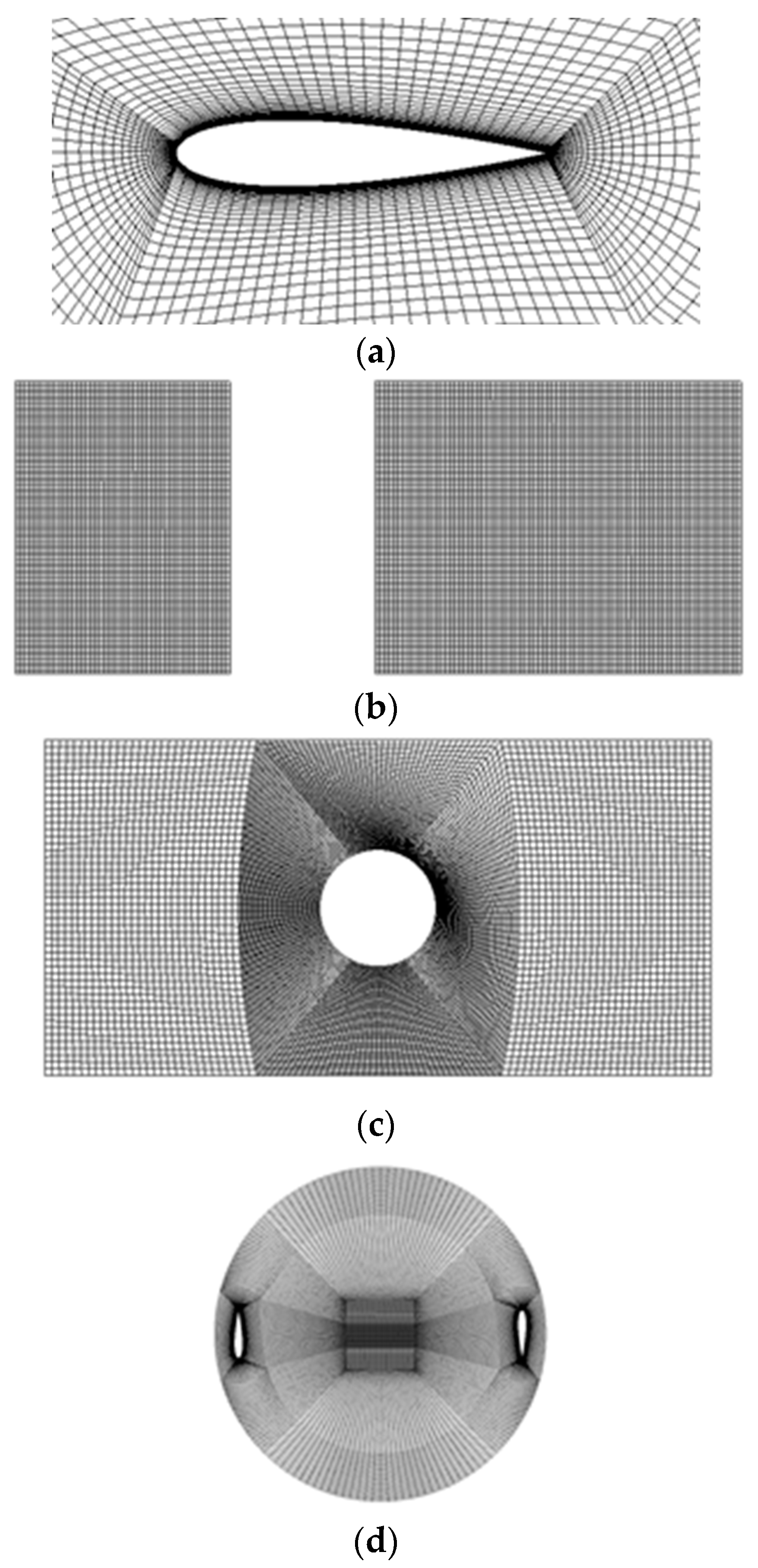
The boundary conditions are set as follows. The standard atmospheric pressure is chosen as the reference pressure. The velocity and turbulence intensity of the inflow are set in the velocity inlet boundary. The relative pressure at the outlet is zero. The sidewalls are open boundaries where fluid can flow in or out freely. The surface of the blades is assumed to be a non-slip wall. The initial velocity of the whole fluid domain is VA. The boundary conditions of the whole flow domain are illustrated in Figure 5, while Figure 6 illustrates the details of meshes in sub-domains.
Besides, to ensure the simulation accuracy, the mesh size around the blades should be chosen carefully and Y-plus (Length Scale for the Turbulence) should be in the range from 0.1 to 10. Figure 4 shows the details of the turbine model. The total grid number is 2.32 × 10⁵.
The Shear Stress Turbulence (SST) turbulent model is applied to simulate the turbulent flow field. The SST model was used in the solution process and is a well-tested model combining and . Details of the model can be found in previous papers [31,32]. The velocity loss and turbulence condition of the wake region properties of the turbine are not the main concern of the paper. Therefore, the SST turbulence model was chosen in this simulation. Details of the difference between the two models in the numerical simulation of a tidal turbine can be found in the paper by Ahmed et al. [33]. Auto wall functions are selected in CFX for the sidewalls and the simultaneous solver is chosen for the solution process [34].
RMS (Root Mean Square) is chosen as the convergence control criteria [35]. The default value of the residual target is 1.5 × 10⁻⁴. In the transient simulation setup adopted in this manuscript, the transient solver is used. The minimum number of coefficient loops is four at each time step. Adaptive time steps are chosen in the solution process. The time step is set to 1.0 × 10⁻³ s. The maximum number of coefficient loops within each time step is 15. Detailed discussions of the validation of the time step are shown in Section 3.2. The high resolution second-order backward Euler scheme is used in the transient scheme option.
3. Validation of CFX Results
3.1. Validation of Grid Independence
In order to maintain a balance between numerical results’ accuracy and solution time, the mesh quality should be carefully decided. A higher mesh quality will describe the physical characteristics of the model precisely, but it will require many more computing resources and take a longer time. Therefore, the mesh quality should take the time consumption and accuracy into consideration. Three different meshes (Table 2) are chosen to validate the mesh independence.
As is shown in Figure 7, the three different meshes have a good match with each other. However, obvious deviation can be seen when the phase angle ranges from 150°–210°. The torque coefficients of mesh 2 and mesh 3 are in good agreement with each other. The torque coefficient changes very little when the Y+ continues decreasing (from mesh 2 to mesh 3). Therefore, the density of mesh 2 can meet the mesh independence requirements in the numerical simulation. The detailed parameters of mesh 2 in Table 2 are adopted in the simulation process.
3.2. Validation of Time Step
Proper time steps play an important role in the solution process. The time steps should also maintain a balance between the accuracy of results and solution time. Therefore, three different time steps were selected to validate the independence of time steps. Figure 8 shows the torque coefficient variation tendency of the VACT in a single period. As Figure 8 shows, the two torque coefficent curves (0.001 s and 0.0005 s) are in good agreement with each other in a period. A longer solution time will occur for 0.0005 s, while the accuracy of 0.0005 s is the same as 0.001 s. Therefore, 0.001 s was chosen in the time steps setup.
3.3. Comparision between Experiments and Numerical Simulation
As is shown in Figure 9, an experiment was carried out in the Circulation Water Tunnel of HEU with a two-bladed VACT. A few key parameters of the adopted VACT are shown in Table 3. The main dimensions of the Circulation Water Tunnel are 8 m × 1.7 m × 1.5 m. The incoming uniform current speed is 0.2 m/s~2 m/s. The experimental results of the power output at different TSR values were compared with the numerical results to verify the feasibility of the 2D simulation method.
The energy utilization coefficient CP is obtained by Equation (13) in Section 2.1. As is shown in Figure 10, exp represents the value of experimental results. Sim represents the value of CFX simulation results. Previous papers [36,37,38] gave the scale coefficient at different arm installation locations and also gave the correlation between turbine span length and maximum power efficiency. The ratio between the span and radius of the turbine used in this experiment is 1.5. Li and Calisal pointed out that the power output could decrease as much as 19.5% in a numerical simulation when the ratio between the span and radius is 1.5. The arm used in this turbine can lead to a decrease of the power output as high as 20%. The cor curve represents the correction curve of sim according to the referenced research results.
As Figure 10 shows, the power efficiency of numerical results is larger than the experimental values. The deviations between numerical and experimental values are mainly caused by the fact that the spoke effect, sidewall effects, and 3D effects are neglected in the numerical simulation. Researchers have carried out experiments and numerical simulations to investigate the effect of the above three factors on the hydrodynamic perfermance of the current turbine. As we can see, the two curves, exp and cor, have the same trend and their peak values are located at the same λ, which is similar to the results obtained by Li and Calisal [37].
In order to further validate the feasibility and accuracy of the proposed 2D method in predicting the turbine load coefficients, a VAWT experiment carried out by Strikland is also used to perform the validation. Water was used as the working medium for the sake of observing the flow field around the turbine blade. Table 4 shows the detailed parameters of the VAWT used in the experiment.
Figure 11a gives the variation tendency of the turbine normal force coefficient for the experiment and numerical simulation in a period. Figure 11b gives the variation tendency of the turbine tangential force coefficient for the experiment and numerical simulation in a period. As we can see, the cyclic variation tendency is in good agreement for the experiment and numerical simulation. There is some difference when the angle ranges from 180°~360°. A similar difference could be seen in the experiment of Strickland et al. They explained in the paper that the deviation ranging from 180°–360° was caused by the mounting error of the blade in their experiment [39]. Apart from the explanation of Strickland et al., the blocking effect caused by the main shaft also changes the flow field, thus leading to the deviation between the experiment and numerical simulation. The vortex shedding of the upstream disk also results in the turbulent flow in the downstream during the phase angle range. This could also be one of the causes of the deviation. Nevertheless, the cyclic variation tendency is in good agreement for exp and cal. The 2D numerical method can be used to predict the turbine load conditions and power out.
4. Results from Hydrodynamic Analysis of the Rotor Under Forced Oscillation
4.1. Flow Field Analysis Under Forced Oscillation
The development of the wake of the turbine in uniform flow without oscillation is shown in Figure 12a. The wake behind the blade is rotated due to the rotational motion of the blade. Meanwhile, the wake flow field develops and the magnitude of vortex decreases along the inflow direction.
Figure 12b illustrates the distribution of wake intensity in the flow field when the turbine is under forced oscillation in sway. Compared with Figure 12a, the wake in Figure 12b moves in the direction perpendicular to the inflow direction and the wake looks like the Von Karman vortex street.
If the turbine oscillates in the surge direction, the distance between the vortex changes along the oscillation motion. When the turbine moves along the incident flow, the distance between the vortex increases (shown in Figure 12c), but the distance between the vortex decreases when the turbine moves against the incident flow (shown in Figure 12d). In the latter case, the turbine is in the wake developing area. The interaction between the turbine and the wake is strong, thus leading to the fact that the flow field within the rotor plane becomes turbulent.
4.2. Analysis of Loads on the Rotor of the Turbine
Fluctuations of the loads acting on the rotor of the turbine have significant effects on the rotor and the main shaft, particularly in terms of structural strength and fatigue life, which affects the safety and reliability of the turbine.
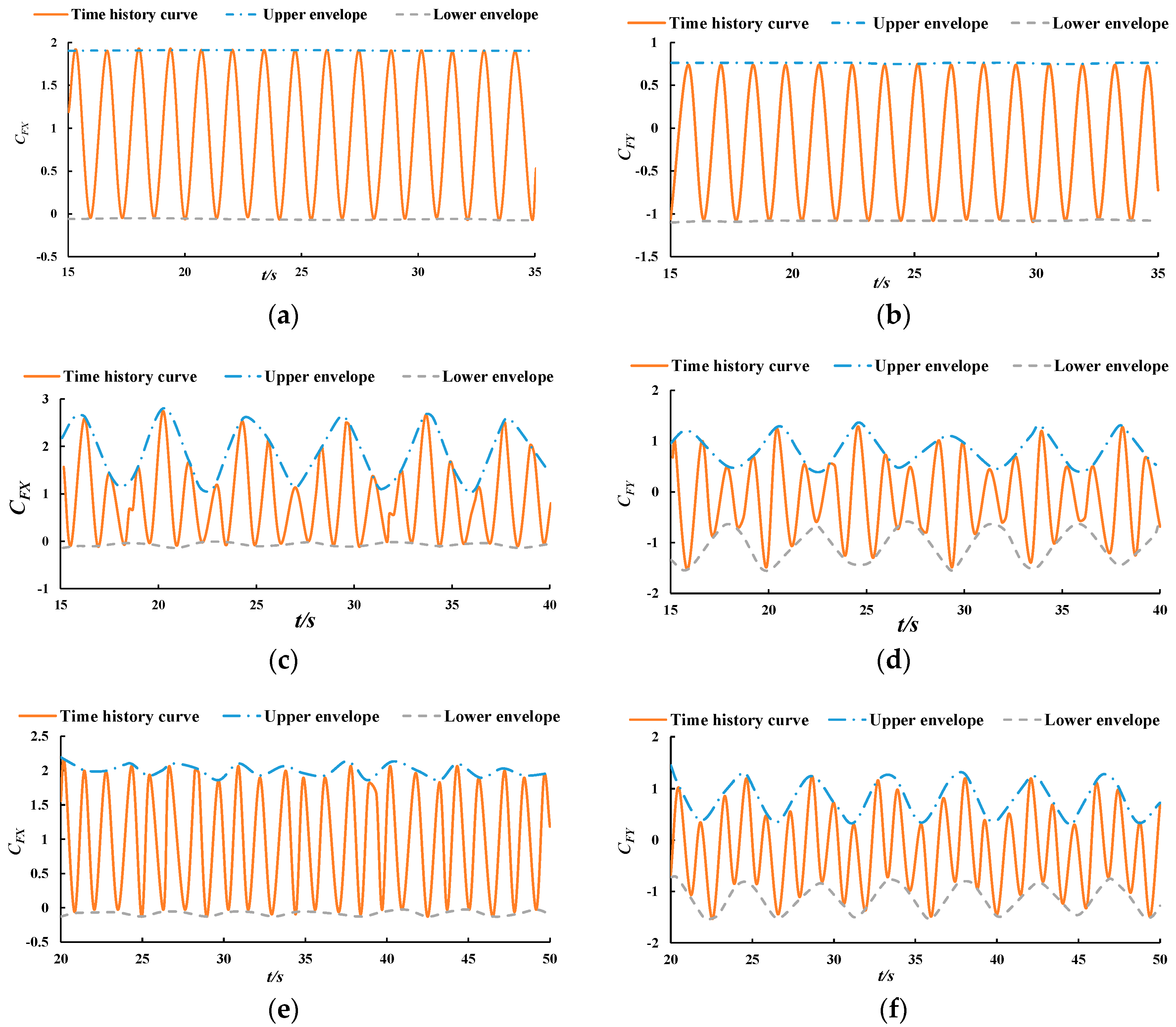
Figure 13a,b illustrate the load curves of the static turbine under the condition = 3.5 m/s and = 2.0. The loads are periodic and fluctuate with the rotation of the turbine. The peak values are respectively constant. Additionally, the envelopes of the peak value curves are horizontal straight lines.
However, the results are quite different when the turbine is under forced oscillation in the plane. The turbine oscillates according to . The oscillating velocity of the turbine would be . The oscillating frequency is = 1.0 rad/s and the oscillating amplitude is = 0.6 m. The biggest oscillating velocity would be = 0.6 m/s, whic is less than the incoming flow velocity. The velocity of the inflow is = 3.5 m/s and the TSR of the rotor is = 2.0. The load curves of the rotor are shown in Figure 13c–f. The peak values of the load acting on the rotor fluctuate along time. Furthermore, the envelope of the peak value load curve is periodic and fluctuates with the oscillation of the turbine. The rotational frequency of the rotor is = 2.332 rad/s and it is much larger than the oscillating frequency = 1.0 rad/s. The variation of the load curves is mainly influenced by the rotational frequency of the turbine. Therefore, the fluctuation of the loads can be divided into two parts when the rotor is under forced oscillation in a single degree of freedom. The first part is the low-frequency part related to the oscillating frequency and the other part is the high-frequency part related to the rotational frequency. The envelopes of the load curves represent the change trends of loads on the rotor when the rotor is under forced oscillation. As we can see from Figure 13c–f, the fluctuations of the loads are stronger when the rotor is under forced oscillation.
4.3. Analysis of Loads on the Blade of the Rotor
The loads acting on the blades are determined by the relative inflow velocity on the blades. When the rotor is under forced oscillation, the relative inflow velocity will change and the loads acting on the blades will also change.
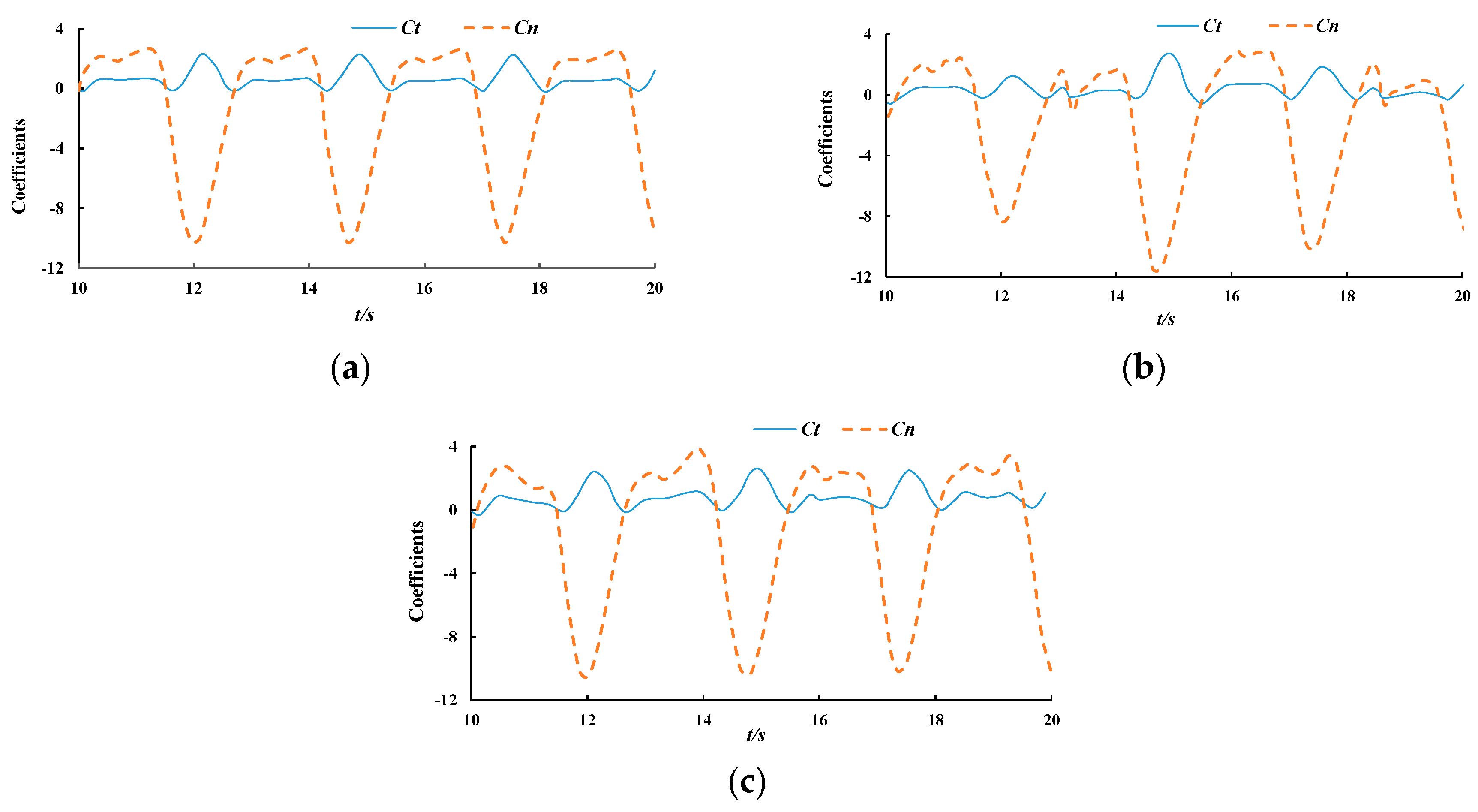
The three figures in Figure 14 illustrate the normal and tangential force coefficients of the blades when the inflow velocity is VA = 3.5 m/s and λ = 2.0. Meanwhile, the rotor oscillates with the amplitude ξ0 = 0.6 m and frequency ωe = 0.2 rad/s. As Figure 14c shows, the normal force coefficient is larger than the tangential force coefficient, which means that the normal force is the dominant part of the loads acting on the blade. Under an oscillation condition, the cyclic variation trend of the normal force curve and the tangential force coefficient curve is similar to the trend without oscillation, but the peak values change due to oscillation.
4.4. Effects of Oscillating Frequency
According to Equations (22) and (23), represents the mean thrust of the rotor and is the amplitude of fluctuation of the thrust. Figure 15 shows that and remain constant, but their amplitudes ( and ) increase linearly with the growth of frequency of oscillation. The value of under the oscillating frequency = 2.0 rad/s is 80% higher than the value without oscillation. This means that the loads acting on the rotor will fluctuate with a high frequency and will encounter a larger amplitude when the rotor encounters high frequency waves in real sea. This would be a challenge for the structural characteristics of the rotor. However, further research is needed on the hydrodynamic characteristics of the rotor when the oscillating frequency is close to the natural frequency of the floater.
4.5. Effects of Oscillating Amplitude
Different oscillation amplitudes ( = 0.2 m~2.0 m) are selected to study how oscillation amplitude affects the hydrodynamic performance of the turbine. The velocity of the incident flow is = 3.5 m/s and the tip speed ratio is λ = 2.0. The oscillating frequency and amplitude are, respectively, = 1.0 rad/s and . The time-averaged value and amplitude of the force coefficient of the rotor are shown in Figure 16. and remain constant when the oscillating frequency is changed. However, and increase linearly with the growth of oscillating amplitude. The value of reaches 2.2 when the amplitude of surge oscillation is = 2.0 m and it is over twice as large as the value under a non-oscillating condition. This means that it is of great importance to reduce the motion amplitude of the turbine considering the aspects of structural strength and fatigue life.
4.6. Analysis of Torque
Figure 17 shows how the torque coefficient of the rotor changes with the oscillating frequency and amplitude when is 3.5 m/s and λ is 2.0. The mean value of the torque coefficient does not change much according to the oscillation frequency in the surge and sway direction. However, the fluctuation of the torque coefficient in surge oscillation is more severe than in sway oscillation. Specifically, the amplitude of the torque coefficient in surge oscillation is twice as large as that in sway oscillation. This is caused by the fact that the turbine in surge motion will encounter the wake of the field, thus leading to rapidly relative velocity change within the turbine disk. Therefore, the hydrodynamic loads fluctuate tempestuously. The fluctuation of torque affects the shaft structural strength and reduces the fatigue life. It also has negative effects on the electric control system and the floater of the turbine.
5. Discussion and Conclusions
Basing on the viscous Computational Fluid Dynamic theories and commercial software CFX, this paper validates the effectiveness of using the proposed CFD procedure to numerically simulate the hydrodynamic performance of VACT under forced oscillation motion. Sliding mesh and moving mesh techiques are applied to simulate the rotation and oscillation of the turbine in unbounded uniform flow. Several numerical validation examples are performed to decide the right mesh size and time step size, which can make the simulation results more accurate, independent, and cost effective. The two-dimensional RANS CFD model is validated with a Darriesus rotor, whose experimental data are available in the literature. The vertical axis current turbine under different oscillation amplitudes and frequencies is simulated with the proposed method. The following conclusions are obtained. The numerical results of the hydrodynamic performance from the two-dimensional numerical simulation method in CFX are in good agreement with experimental results in the literature. It proves that the proposed numerical method could be adopted to investigate the turbine load condition and power output of VACT under forced oscillation. The oscillation frequency is smaller than that of rotation frequency in the numerical simulation. Therefore, the fluctuation of the loads acting on the rotor of the turbine can then be divided into two parts. The low frequency part is connected with the oscillation frequency. The high frequency part is connected with the rotational frequency of the rotor. Compared with the non-oscillating case, the time-averaged values of the loads acting on the rotor change little, while the fluctuation amplitudes of these loads display significant changes. The oscillation of the turbine causes larger amplitude of cyclic variation of the load coefficients. The unobvious variations of mean turbine loads coefficients lie in the fact that the velocity change on the turbine disk is periodic. The mean velocity change within the turbine disk in a period is 0. The fluctuation amplitudes of these loads (normal force, tangential force, toruqe, thrust) increase linearly with the growth of oscillating frequency and amplitude. The mean value of the torque coefficient of the rotor remains constant under forced oscillation motion, but the fluctuation of the instantaneous torque coefficient is obvious. The fluctuation amplitude of the normal and tangential force coefficient induced by forced surge oscillation is twice as large as the fluctuation amplitue induced by forced sway oscillation. The cause of this phenomenon lies in the fact that the turbine may move to the wake area in the surge motion. The turbulence in the wake area leads to rapid velocity change within the turbine disk area, which causes bigger fluctuation in blade loads and torque. It can be observed that the wake generated in the forced sway oscillation is similar to the Von Karman vortex street. The distance between the vortex changes when the turbine is in surge motion. The oscillation frequency has more influence on the frequency of vortex leakage, while the oscillation frequency has more influence on the length of the wake area.
The current research adopted a 2D numerical method to study the hydrodynamic performance of the vertical axis current turbine under forced oscillation. Several limitations of this method should be clearly stated. We assume that the immersion depth is deep enough, thus, the waves would not have influence on the flow velocity passing through the turbine disk. In a 2D numerical simulation, the default value of water depth is infinite. When the linear incoming wave frequency is , the theoretical value of the required immersion depth would be . The actual immersion depth of a turbine installed on a floater would be limited. The vertical component of wave velocity of waves might interact three-dimensionally with the flow around the turbine, which would make the problem more complicated. Therefore, the accuracy of the proposed method would be reduced when the turbine encounters long waves, since the immersion depth can no longer be guaranteed. Moreover, the realistic wave conditions for a sea enviroment would seldomly be regular and unidirectional. The irregular waves will most likely reduce the efficiency of the turbine.
The results of this manuscript can provide a valuable reference for study on the hydrodynamic performance of VACTs subjected to wave-induced motion. The power output efficiencies of the vertical axis current turbine under different oscillation frequencies and oscillation amplitues are systematically analysed. Besides, the turbine blade would experience higher fluctuation for blade force under oscillation. The oscillation of the turbine would increase the intantanous load, but the average load would change little. The analysis results of the blade coefficient can also guide structure strength design and fatigue life analysis.
Author Contributions
Conceptualization, C.H. and M.Y.; Methodology, Y.L.; Software, C.H.; Validation, C.H. and M.Y.; Investigation, Y.M.; Resources, Y.M.; Data Curation, C.H.; Writing-Original Draft Preparation, C.H.; Writing-Review & Editing, C.H.; Visualization, C.H.; Supervision, R.D.; Project Administration, Y.M.; Funding Acquisition, Y.M.
Funding
This paper was financially supported by the National Natural Science Foundation of China (Grant No.51779062; 51579055), the Fundamental Research Funds for the Central Universities of China (No.HEUCFP201714), Shenzhen Special Fund for Future Industries (No. JCYJ20160331163751413).
Acknowledgments
We acknowledge the support of the colleges from Institute of Marine Renewable Energy in Harbin Engineering University. We would also like to give thanks to Li Lei from CIMC Offshore Ltd for his investigation support.
Conflicts of Interest
The authors declare no conflict of interest.
Nomenclature
| Incoming flow velocity | |
| Lift force of a single blade | |
| Drag force of a single blade | |
| Torque acting on the o axis of the airfoil | |
| Force along the chord line | |
| Force perpendicular to the chord line | |
| Blade tangential force | |
| Radial blade force | |
| Thrust of the rotor | |
| Lateral force of the rotor | |
| Torque of a single blade | |
| SST | Shear Stress Turbulence |
| N-S | Navier-Stokes |
| LES | Large eddy simulation |
| RANS | Reynolds-averaged Navier–Stokes |
| Y plus | Dimensionless wall distance |
| CEL | Computer expression language |
| Cp | Power output efficiency |
| Mean thrust of the rotor | |
| Fluctuation of the amplitude | |
| Solidarity of the turbine | |
| TSR | Tip speed ratio |
| MCT | marine current turbine |
| VAW | Ts vertical axis wind turbines |
References
- Rourke, F.O.; Boyle, F.; Reynolds, A. Tidal energy update 2009. Appl. Energy 2010, 87, 398–409. [Google Scholar] [CrossRef]
- Bahaj, A.B.S. Generating electricity from the oceans. Renew. Sustain. Energy Rev. 2011, 15, 3399–3416. [Google Scholar] [CrossRef]
- Magagna, D.; Margheritini, L.; Alessi, A.; Bannon, E.; Boelman, E.; Bould, D.; Coy, V.; De Marchi, E.; Frigaard, P.; Guedes Soares, C.; et al. Workshop on Identification of Future Emerging Technologies in the Ocean Energy Sector—27th March 2018, Ispra, Italy; EUR29315 EN; European Commission: Luxembourg, 2018; ISBN 978-92-79-92587-0. [Google Scholar]
- Jun, D.; Zhong, S.H.; Xi, W.; Jie, Y. Current research progress of water turbine. Renew. Energy 2010, 28, 130–133. [Google Scholar]
- Denny, E. The economics of tidal energy. Energy Policy 2009, 37, 1914–1924. [Google Scholar] [CrossRef]
- Mehmood, N. Tidal current technologies: Green and renewable. In Proceedings of the 2011 4th IEEE International Conference on Computer Science and Information Technology (ICCSIT2011), Chengdu, China, 10–12 June 2011. [Google Scholar]
- Sheng, Q.-H.; Tang, F.-D.; Wang, H.-F.; Cao, X.-F.; Zhao, W.-M.; Jin, Z.-G.; Han, D.-F.; Zhang, L. The design of 2 × 150 kW floating vertical-axis tidal current independent generating system. In Proceedings of the Symposium of the 16th China Marine (Coastal) Engineering Symposia, Dalian, China, 4–7 August 2013; pp. 758–763. [Google Scholar]
- Zhang, L.; Wang, L.-B.; Li, F.-L. Streamtube models for performance prediction of vertical-axis variable-pitch turbine for tidal current energy conversion. J. Harbin Eng. Univ. 2004, 25, 261–266. [Google Scholar]
- Yang, B.; Shu, X.-W. Hydrofoil optimization and experimental validation in helical vertical axis turbine for power generation from marine current. Ocean Eng. 2012, 42, 35–46. [Google Scholar] [CrossRef]
- Bahaj, A.S.; Batten, W.M.J.; McCann, G. Experimental verifications of numerical predictions for the hydrodynamic performance of a horizontal axis marine current turbines. Renew. Energy 2007, 32, 2479–2490. [Google Scholar] [CrossRef]
- Mccann, G.; Rawlinson, R.; Garrad, H.; Partners Ltd. (Bristol UK). Development of a design tool for current turbines. Smith, 2005. [Google Scholar]
- Batten, W.M.; Bahaj, A.S.; Molland, A.F.; Chaplin, J.R. The prediction of the hydrodynamic performance of marine current turbines. Renew. Energy 2008, 33, 1085–1096. [Google Scholar] [CrossRef]
- Maganga, F.; Germain, G.; King, J.; Pinon, G.; Rivoalen, E. Experimental characterization of flow effects on marine current turbine behavior and on its wake properties. IET Renew. Power Gen. 2010, 4, 498–509. [Google Scholar] [CrossRef]
- Lust, E.E.; Luznik, L.; Flack, K.A.; Walker, J.M.; Van Benthem, M.C. The influence of surface gravity waves on marine current turbine performance. Int. J. Mar. Energy 2013, 3, 27–40. [Google Scholar] [CrossRef]
- Fernandez-Rodriguez, E.; Stallard, T.J.; Stansby, P.K. Experimental study of extreme thrust on a tidal stream rotor due to turbulent flow and with opposing waves. J. Fluids Struct. 2014, 51, 354–361. [Google Scholar] [CrossRef]
- Ai, K.; Avital, E.J.; Korakianitis, T.; Samad, A.; Venkatesan, N. Surface wave effect on marine current turbine, modelling and analysis. In Proceedings of the International Conference on Mechanical and Aerospace Engineering, London, UK, 18–22 July 2016; pp. 180–184. [Google Scholar]
- Guo, X.; Gao, Z.; Yang, J.; Moan, T.; Lu, H.; Li, X.; Lu, W. The Effects of Surface Waves and Submergence on the Performance and Loading of a Tidal Turbine. In Proceedings of the International Conference on Ocean, Offshore and Arctic Engineering (ASME 2017), Trondheim, Norway, 25–30 June 2017; p. V07BT06A055. [Google Scholar]
- Yan, J.; Deng, X.; Korobenko, A.; Bazilevs, Y. Free-surface flow modeling and simulation of horizontal-axis tidal-stream turbines. Comput. Fluids 2017, 158, 157–166. [Google Scholar] [CrossRef]
- Ansys Inc. ANSYS CFX; Ansys Inc.: Canonsburg, PA, USA, 2015. [Google Scholar]
- Lanzafame, R.; Mauro, S.; Messina, M. 2D CFD Modeling of H-Darrieus Wind Turbines Using a Transition Turbulence Model. Energy Procedia 2014, 45, 131–140. [Google Scholar] [CrossRef]
- Lam, H.F.; Peng, H.Y. Study of wake characteristics of a vertical axis wind turbine by two- and three-dimensional computational fluid dynamics simulations. Renew. Energy 2016, 90, 386–398. [Google Scholar] [CrossRef]
- Ferreira, C.S.; Bussel, G.V.; Kuik, G.V. 2D CFD Simulation of Dynamic Stall on a Vertical Axis Wind Turbine: Verification and Validation with PIV Measurements. In Proceedings of the 45th AIAA Aerospace Sciences Meeting and Exhibit, Reno, NV, USA, 8–11 January 2007. [Google Scholar]
- Danao, L.A.; Howell, R. Effects on the Performance of Vertical Axis Wind Turbines with Unsteady Wind Inflow: A Numerical Study. In Proceedings of the AIAA Aerospace Sciences Meeting Including the New Horizons Forum and Aerospace Exposition, Nashville, TN, USA, 9–12 January 2012. [Google Scholar]
- Migliore, P.G. Comparison of NACA 6-series and 4-digit airfoils for Darrieus wind turbines. J. Energy 1983, 7, 291–292. [Google Scholar] [CrossRef]
- Yang, B.; Lawn, C. Three-dimensional effects on the performance of a vertical axis tidal turbine. Ocean Eng. 2013, 58, 1–10. [Google Scholar] [CrossRef]
- Alidadi, M.; Calisal, S. A numerical method for calculation of power output from ducted vertical axis hydro-current turbines. Comput. Fluids 2014, 105, 76–81. [Google Scholar] [CrossRef]
- Dai, Y.M.; Gardiner, N.; Lam, W.H. CFD modelling strategy of a straight-bladed vertical axis marine current turbine. In Proceedings of the Twentieth International Offshore and Polar Engineering Conference, Beijing, China, 20–25 June 2010. [Google Scholar]
- Wang, L.B.; Zhang, L.; Zeng, N.D. A potential flow 2-D vortex panel model: Applications to vertical axis straight blade tidal turbine. Energy Convers. Manag. 2007, 48, 454–461. [Google Scholar] [CrossRef]
- Yang, Z.; Deng, B.Q.; Shen, L. Direct numerical simulation of wind turbulence over breaking waves. J. Fluid Mech. 2018, 850, 120–155. [Google Scholar] [CrossRef]
- Alberello, A.; Pakodzi, C.; Nelli, F.; Bitner-Gregersen, E.M.; Toffoli, A. Three dimensional velocity field underneath a breaking rogue wave. In Proceedings of the OMAE, Trondheim, Norway, 25–30 June 2017. [Google Scholar]
- Menter, F. Two-equation eddy-viscosity turbulence models for engineering applications. AIAA J. 1994, 32, 1598–1605. [Google Scholar] [CrossRef] [Green Version]
- Scardovelli, R.; Zaleski, S. Direct numerical simulation of free-surface and interfacial flow. Annu. Rev. Fluid Mech. 1999, 31, 567–603. [Google Scholar] [CrossRef]
- Ahmed, U.; Apsley, D.D.; Afgan, I.; Stallard, T.; Stansby, P.K. Fluctuating Loads on a Tidal Turbine Due to Velocity Shear and Turbulence: Comparison of CFD with Field Data. Renew. Energy 2017, 112, 235–246. [Google Scholar] [CrossRef]
- Mooney, K.G.; Maric, T.; Hopken, J. The OpenFOAM Technology Primer; Source flux: Duisburg, Germany, 2014. [Google Scholar]
- Ma, Y.; Hu, C.; Li, Y.; Li, L.; Deng, R.; Jiang, D. Hydrodynamic Performance Analysis of the Vertical Axis Twin-Rotor Tidal Current Turbine. Water 2018, 10, 1694. [Google Scholar] [CrossRef]
- Marsh, P.; Ranmuthugala, D.; Penesis, I.; Thomas, G. Three-dimensional numerical simulations of straight-bladed vertical axis tidal turbines investigating power output, torque ripple and mounting forces. Renew. Energy 2015, 83, 67–77. [Google Scholar] [CrossRef] [Green Version]
- Li, Y.; Calisal, S.M. Three-dimensional effects and arm effects on modeling a vertical axis current turbine. Renew. Energy 2010, 35, 2325–2334. [Google Scholar] [CrossRef]
- Marsh, P.; Ranmuthugala, D.; Penesis, I.; Thomas, G. The influence of turbulence model and two and three-dimensional domain selection on the simulated performance characteristics of vertical axis tidal turbines. Renew. Energy 2017, 105, 106–116. [Google Scholar] [CrossRef] [Green Version]
- Strickland, J.H.; Webster, B.T.; Nguyen, T. A vortex model of the Darrieus turbine: An analytical and Experimental Study. J. Fluids Eng. 1979, 101, 500–505. [Google Scholar] [CrossRef]
Figure 1.
2 × 150 kW floating vertical current turbine system.

Figure 2.
2 × 300 kW floating vertical current turbine system.

Figure 3.
Coordinate and force on the blade-section (top view of the turbine blade).

Figure 4.
Motion of a vertical-axis current turbine in a wave condition.

Figure 5.
Sub-domains and boundary conditions for simulation of forced oscillation in surge. (a) Sub-domains for simulation of forced oscillation in surge. (b) Boundary conditions.
Figure 5.
Sub-domains and boundary conditions for simulation of forced oscillation in surge. (a) Sub-domains for simulation of forced oscillation in surge. (b) Boundary conditions.


Figure 6.
Meshes in sub-domains. (a) Meshes around blades. (b) Meshes in stationary domain. (c) Meshes in oscillatory domain and stationary domain. (d) Meshes in rotational domain.
Figure 6.
Meshes in sub-domains. (a) Meshes around blades. (b) Meshes in stationary domain. (c) Meshes in oscillatory domain and stationary domain. (d) Meshes in rotational domain.

Figure 7.
Torque coefficient variation tendency for different mesh densities.

Figure 8.
Torque coefficient variation tendency for different timesteps.

Figure 9.
Experimental equipment. (a) Circulation Water Tunnel. (b) Supporting Platform. (c) Two-bladed vertical axis turbine.
Figure 9.
Experimental equipment. (a) Circulation Water Tunnel. (b) Supporting Platform. (c) Two-bladed vertical axis turbine.

Figure 10.
CP from numerical simulation and from experiment.

Figure 11.
Comparison between experiement and numerical simulation results. (a) Turbine normal force coefficient. (b) Turbine tangential force coefficient.
Figure 11.
Comparison between experiement and numerical simulation results. (a) Turbine normal force coefficient. (b) Turbine tangential force coefficient.

Figure 12.
Cloud distribution of vortex in the flow field of the turbine. (a) Cloud distribution of vortex when the turbine only rotates. (b) Cloud distribution of vortex when the turbine rotates under forced oscillation in sway. (c) Cloud distribution of vortex when the turbine moves along the incident flow. (d) Cloud distribution of vortex when the turbine moves against the incident flow.

Figure 13.
Load curves of the rotor. (a) Thrust coefficient of the rotor when it does not oscillate. (b) Coefficient of tangential force when the rotor does not oscillate. (c) Thrust coefficient of the rotor when it oscillates in surge. (d) Coefficient of tangential force when the rotor oscillates in surge. (e) Thrust coefficient of the rotor when it oscillates in sway. (f) Coefficient of tangential force when the rotor oscillates in sway.

Figure 14.
Normal and tangential force coefficient of one blade. (a) Normal and tangential force coefficient of one blade when the rotor is static. (b) Normal and tangential force coefficient of one blade when the rotor is in surge motion. (c) Normal and tangential force coefficient of one blade when the rotor is in sway motion.

Figure 15.
Time-averaged value and amplitude of load coefficients of the rotor vs. oscillating frequency. (a) Time-averaged value and amplitude of load coefficients of the rotor under surge oscillation. (b) Time-averaged value and amplitude of load coefficients of the rotor under sway oscillation.
Figure 15.
Time-averaged value and amplitude of load coefficients of the rotor vs. oscillating frequency. (a) Time-averaged value and amplitude of load coefficients of the rotor under surge oscillation. (b) Time-averaged value and amplitude of load coefficients of the rotor under sway oscillation.

Figure 16.
Time-averaged value and amplitude of load coefficients of the rotor vs. oscillating amplitude. (a) Time-averaged value and amplitude of load coefficients of the rotor under surge oscillation. (b) Time-averaged value and amplitude of load coefficients of the rotor under sway oscillation.
Figure 16.
Time-averaged value and amplitude of load coefficients of the rotor vs. oscillating amplitude. (a) Time-averaged value and amplitude of load coefficients of the rotor under surge oscillation. (b) Time-averaged value and amplitude of load coefficients of the rotor under sway oscillation.

Figure 17.
Time-averaged value and amplitude of the torque coefficient of the rotor. (a) Effects of oscillating frequency. (b) Effects of oscillating amplitude.
Figure 17.
Time-averaged value and amplitude of the torque coefficient of the rotor. (a) Effects of oscillating frequency. (b) Effects of oscillating amplitude.


Table 1.
Detailed parameters of the Vertical Axis Current turbine (VACT).
| Number of Blades | Turbine Diameter (m) | Chord Length (m) | Aspect Ratio | Compactness |
|---|---|---|---|---|
| 2 | 6 | 0.9 | 6.5 | 0.0955 |
Table 2.
Detailed mesh information.
| Mesh | Total Mesh Quantity (×103) | Y+ | Solution Time | Total Boundary Mesh Layer | Thickness of the First Layer |
|---|---|---|---|---|---|
| 1 | 45 | 21.5–38.2 | 4 h | 30 | 0.0004 m |
| 2 | 119 | 2.65–4.76 | 12 h | 30 | 0.0001 m |
| 3 | 274 | 0.83–1.96 | 26 h | 30 | 0.00005 m |
Table 3.
Detailed parameters in the experiment.
| Diameter (m) | Numer of Blades | Cord Length (m) | Air Foil | Aspect Ratio |
|---|---|---|---|---|
| 0.8 m | 2 | 0.12 | NACA0018 | 1.5 |
Table 4.
Detailed parameters of Strikland turbine.
| Diameter D/m | Blades Number Z | Chord Length C/m | Airfoil | Rotation Speed /rad−1 |
|---|---|---|---|---|
| 1.22 | 2 | 0.0914 | NACA0012 | 0.749 |
© 2018 by the authors. Licensee MDPI, Basel, Switzerland. This article is an open access article distributed under the terms and conditions of the Creative Commons Attribution (CC BY) license (http://creativecommons.org/licenses/by/4.0/).
Share and Cite
MDPI and ACS Style
Ma, Y.; Hu, C.; Li, Y.; Deng, R. Research on the Hydrodynamic Performance of a Vertical Axis Current Turbine with Forced Oscillation. Energies 2018, 11, 3349. https://doi.org/10.3390/en11123349
AMA Style
Ma Y, Hu C, Li Y, Deng R. Research on the Hydrodynamic Performance of a Vertical Axis Current Turbine with Forced Oscillation. Energies. 2018; 11(12):3349. https://doi.org/10.3390/en11123349
Chicago/Turabian StyleMa, Yong, Chao Hu, Yulong Li, and Rui Deng. 2018. "Research on the Hydrodynamic Performance of a Vertical Axis Current Turbine with Forced Oscillation" Energies 11, no. 12: 3349. https://doi.org/10.3390/en11123349
Note that from the first issue of 2016, this journal uses article numbers instead of page numbers. See further details here.