Reactive Power Optimal Control of a Wind Farm for Minimizing Collector System Losses


1
Department of Control and Computer Engineering, North China Electric Power University, Beijing 102206, China
2
North China Electric Power Research Institute Co., Ltd., Beijing 100032, China
*
Author to whom correspondence should be addressed.
Energies 2018, 11(11), 3177; https://doi.org/10.3390/en11113177
Submission received: 17 October 2018
/
Revised: 6 November 2018
/
Accepted: 13 November 2018
/
Published: 16 November 2018
(This article belongs to the Section F: Electrical Engineering)
Abstract
:A reactive power/voltage control strategy is proposed that uses wind turbines as distributed reactive power sources to optimize the power flow in large-scale wind farms and reduce the overall losses of the collector system. A mathematical model of loss optimization for the wind farm collector systems is proposed based on a reactive power/voltage sensitivity analysis; a genetic algorithm (GA) and particle swarm optimization (PSO) algorithm are used to validate the optimization performances. The simulation model is established based on a large-scale wind farm. The results of multiple scenarios show that the proposed strategy is superior to the traditional methods with regard to the reactive power/voltage control of the wind farm and the loss reduction of the collector system. Furthermore, the advantages in terms of annual energy savings and environmental protection are also estimated.
1. Introduction
Due to the advancements in wind generation and the increase in the size of wind farms (WFs), the uncertainty of wind power has a larger impact on the system stability and operational benefits. However, WFs are required to have the ability to support voltage and reactive power at the point of common coupling (PCC) according to the Grid Code, which requires a well-configured reactive power control system [1]. Generally, WFs are equipped with a certain number of reactive power compensation devices such as static volt-ampere reactive compensators (SVCs) and static synchronous compensators (STATCOMs) to ensure voltage stability when a three-phase short circuit and other various faults occur [2,3]. Some researchers have enhanced the voltage stability of each bus in the WF via precisely coordinated control in case of a failure [4,5]. Nonetheless, this method is not suitable for reactive power dispatching under normal operations because of economic reasons [6].
Currently, the mainstream doubly-fed and direct-driven wind turbine (WT) operates continuously between 0.95 power factor lead and 0.95 lag because both of their converter systems have good reactive power control capability [7]. These WTs could be regarded as reactive power compensation devices that can be flexibly controlled at low costs in WFs. In a large-scale WF, transformers and collector circuits are more abundant than in other power plants, contributing to greater losses [8]. Furthermore, the transmission chain, the converter and other equipment losses are strongly related to the performance of the WT, while the losses in the collector system are significantly influenced by the distribution of the electrical power flow [9]. Therefore, the control of the reactive power of the WTs and the optimization of the load flow are effective methods for improving the voltage level and achieving energy-savings in WFs.
Reducing the line loss through power flow optimization is an important measure for the economic operation of the power system. In reference [10], a robust cone programming approach to determine the ramp power limit with AC power flow constraints was proposed to maximize the total operating range of WFs. In reference [11], the optimal operation model of active distribution networks is established, to reduce the power losses and improve the voltage profiles. Automatic voltage control (AVC) is usually used in reactive power dispatching of large-scale WFs and focuses on improving the voltage control level of WFs [12]. If the loss reduction control of the collector system is also incorporated into the reactive power control goal through load-flow optimization, the operations of the WF and the control performance of the AVC system can be improved.
To address the aforementioned problems, a reactive power control system based on optimal reactive power dispatch (ORPD) in a WF is proposed in this paper. The control variable is the reactive power reference of each WT and is implemented by a sensitivity coefficient matrix with the purpose to reduce the losses in the collector system and maintain the voltage stability of each bus. Simultaneously, this control system satisfies the grid code regarding the reactive power demands of the PCC. The established optimization model is solved using a genetic algorithm (GA) and particle swarm optimization (PSO) algorithm to determine a suitable algorithm for the ORPD. To improve the convergence, the voltage violation is addressed using a penalty function. The proposed dispatch method is compared with the proportional dispatching approach in various cases. The GA and PSO algorithm are both effective for specific WFs, whereas the results of the GA are better for the estimation of the energy-savings for the annual power generation.
The rest of this paper is organized as follows. The architecture of the proposed reactive power control system is described in Section 2. Section 3 presents the GA and PSO algorithm and describes the solution of the optimization search problem. Section 4 shows the test results for verifying the effectiveness of the established optimization model in different cases. Finally, the conclusion is given in Section 5.
2. The Proposed Reactive Power Control System
The architecture of the proposed reactive power control system is shown in Figure 1 and the operation of the system is as follows. First, based on the topology and the parameters of the WTs and collector system, the admittance matrix of the nodes Ybus is created and is used for the power flow analysis under specific wind conditions. A Jacobian matrix J that is calculated based on the load flow deduces the reactive power/voltage sensitivity matrix between the buses and the loss model of the collector system is generated. Second, an optimization model with the objective function of the minimum loss of the collector system is established and the control variable is the reactive power reference of each WT. This model begins with the current working states of each WT and is solved by a random optimization algorithm to obtain the reactive power instruction set.
The flowchart of the dynamic reactive power control system is shown in Figure 2. It communicates with the WF control system-energy management (WFCS-EM) and the cycle control period is designed in minutes. At the same time, the control system provides a mechanism to trigger the control cycle when the wind speed variation exceeds the threshold value. Therefore, this control system meets the real-time requirements of existing WFCS-EM.
2.1. Sensitivity Coefficient Matrix
The loss reduction optimization of the WF collector system must meet the requirements of stable and unlimited voltage at each bus; the reactive power/voltage sensitivity coefficient matrix is established to limit the voltage variation range and improve the optimization efficiency.
The Jacobian matrix of the power system contains the sensitivity information regarding the injection power and voltage of the buses [13]. We consider a WF with n buses of WT, a bus of PCC, and m is the bus to be solved. The Jacobian matrix J in polar coordinates is divided into four parts:
The relationship between the voltage variation and the reactive power variation is as follows:
Consider , that is, only the reactive power of bus m changes. The sensitivity Jacobian matrix of i bus is obtained by a matrix change.
where is the inverse matrix of , A is the specific element of .
The sensitivity relationship between the voltage change of m bus and the reactive power change of j bus is obtained using Equation (5).
2.2. Objective Functions
The collector system of the WF includes transmission lines, the main transformer, and package transformers of the WTs [14]. For the wind farm studied in this paper, the main transformer is a 110 kV/35 kV three-phase step-up transformer connected to the grid, and the package transformer is a 35 kV package integrated compact transformer substation for WT. The optimization model established in this study uses the objective function of the minimum loss in the collector system and the loss model of each part is defined as follows.
● Transformers:
The main transformer and package transformers differ only in terms of the capacity and parameters; their loss models are consistent and can be calculated by Equation (6):
where refers to transformer loss, is the no-load loss, is the load rate, and refers to the load loss.
● Power cables system:
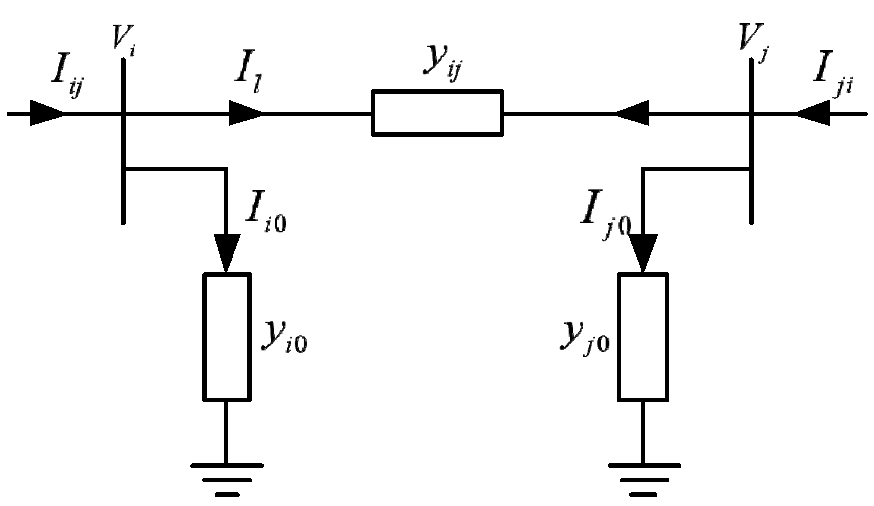
The cables connecting i bus and j bus are shown in Figure 3; y and I represent the admittance and current of each cable, respectively, V represents the voltage of each bus, and the current from i bus to j bus is positive in the i→j direction. The current from i bus to j bus can be calculated using Equation (7).
Similarly, the current from j bus to i bus can be calculated from Equation (8).
The losses in the cable ij are the sum of the complex power:
● The objective function is as follows:
2.3. Constraints
When optimizing the reactive power of the WF, it is necessary to meet not only the constraints of the power flow equation but also the inequality constraints of the reactive power output of the WTs, bus voltage, and apparent power of the lines as follows:
In addition, the reactive power demand at the PCC is also a constraint of this optimization problem:
where represents the reactive power of each WT; indicates the voltage of each bus; and are the reference and measurement values of the reactive power at the PCC, respectively; refers to the apparent power flow in the line l, and n indicates the total number of WTs. The voltage ranges constrain the bus voltage Vj so that it is maintained without violating the allowable region. For the wind farm studied in this paper, each bus voltage is kept between 0.95 pu and 1.05 pu.
3. Algorithm to Solve the Model
The proposed reactive power control strategy is based on the ORPD, which is a multi-objective optimization problem with the characteristics of strong coupling and nonlinearity. Traditional optimization methods such as linear programming, the interior point method [15], and sequential quadratic programming [16] have the characteristics of sensitivity regarding the initial value selection and easy convergence to a locally optimal solution but have difficulty in differentiating the objective function and some other problems; in contrast, a random optimization algorithm is an effective method to solve such problems. However, for specific optimization problems, different random optimization algorithms exhibit differences in convergence speed and global optimization performance. As a result, in this study, we used strategies based on the GA and PSO algorithm separately to verify that the final optimal results are effective.
3.1. Genetic Algorithm
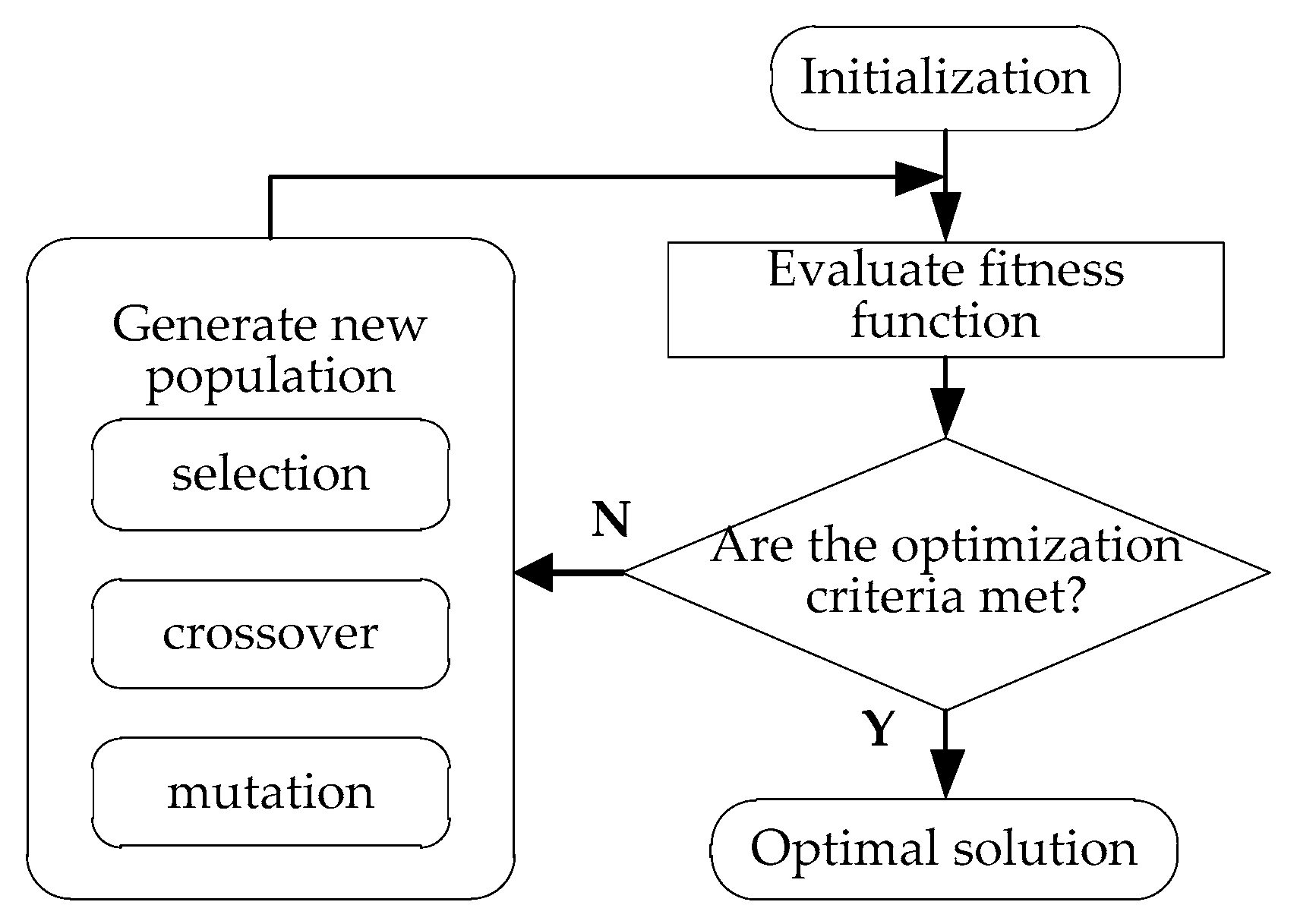
As an evolutionary calculation approach, a GA is probably the most popular method for optimization search problems. A GA is a random search approach based on imitating the process of natural selection; the basic framework of a GA is shown in Figure 4. At the start of the optimization procedure, numerous individuals are initialized at random. Each individual represents a feasible solution. Subsequently, these individuals are estimated using objective functions. The new individuals are subjected to selection, crossover, and mutation. The resulting individuals are selected based on a fitness function to create new offspring [17].
In this study, the original binary-coded GA was extensively modified to effectively address the ORPD problem. First, in the optimization algorithm, the candidate solutions are represented by a combination of floating-point numbers and integers instead of binary strings. Each number in the candidate solution indicates a variable. However, as in the binary-coded GA, every value is regarded as a substring. This representation provides more advantages than the binary code. The computing capability of the GA is greatly improved because it is unnecessary to transform the solution variables into a binary format. In addition, less memory is required. With the combined type of expression, the reproduction operator and evaluation process remain unchanged when the binary-coded GA is used but it is necessary to make some modifications for the crossover and mutation operations. The details on genetic operators applied in the improved GA are described in reference [18].
3.2. Particle Swarm Optimization Algorithm
Particle swarm optimization is based on simulating the foraging behavior of birds. It is also a type of evolutionary algorithm that starts with a random solution, finds the optimal solution by iteration, and evaluates the quality of the solution by a fitness function. However, the PSO has simpler rules than the GA and has no crossover or mutation operations. The PSO algorithm finds a global optimum value by searching for the current best variables in the solution space. Particle swarm optimization algorithms have become popular in recent years due to their high accuracy, fast convergence, and easy implementation. The PSO algorithm is shown in Figure 5. Many researchers have successfully applied PSO algorithms for optimal power flow problems [19]. A comprehensive review of PSO algorithms and applications to power system problems is provided in reference [20].
In this study, the weighted PSO is selected to optimize the proposed ORPD strategy. The parameters of the weighted PSO are the inertia weight w and the acceleration factors C1 and C2. Commonly, the values of C1 and C2 are 2. The inertia weight w controls the exploration of the search space; therefore, an initially higher value (typically 0.9) allows the variables to move freely to find the global optimum neighborhood rapidly. Meanwhile, a lower value of the final inertia weight (usually 0.4) narrows the search and is advantageous for the local search [21]. The inertia weight w that decreases based on a linear function produces good results in many applications; it is calculated using Equation (15).
where is the initial inertia weight, is the final inertia weight, is the current iteration times, is the maximum iteration times.
3.3. Constraints Handling
The constraint handling is a very important part of the optimization problem and directly affects the quality of optimization. We use an identical constraint handling method in the ORPD strategy optimized by the GA and PSO because both methods evaluate the solution using a fitness function. The methods can be classified according to the following four types: search of feasible solutions, penalty function, solution repair method, and hybrid methods.
Because of the random nature of the GA and PSO, some variables may exceed their limitations and may consume more time for the algorithm to converge. Penalty functions are used in this study to ensure that a solution is found and the constraints are met. This penalty function implies that if a variable violates the inequality restraint, it will be subject to a penalty that extends to the objective function. In this study, the penalty functions used for handling the inequality constraints are used in the following manner:
In order to search an optimization solution as soon as possible, the equality constraint in Equation (14) is modified and an error value is included as follows:
As mentioned above, the penalty function is used in the following equation when the variables surpass the limits:
where,
- --
- indicates the control variables involving the reactive power setting of all WTs.
- --
- represents the dependent variables, including all bus voltages and the reference reactive power of the PCC.
- --
- , and are called the penalty factors in this study; they increase gradually and have little influence on the initial iterations.
- --
- is the absolute value of the difference between and .
In addition, the determination of the penalty factor is an important aspect because it affects the final optimization result and the optimal penalty factor value is not always the same under different wind conditions. In this study, the corresponding optimal penalty factor value of each case is obtained using a series of tests, an empirical value method in engineering, multiple test methods, and a comprehensive approach.
4. Case Study
The ORPD strategy is aimed at minimizing the collector system loss in a WF without additional reactive power compensation sources; all the WTs are subject to the same voltage and power. In order to ensure that the voltage does not violate the limits and the active power generation is not influenced by reactive power dispatching, the reactive power demand at the PCC is set in the range of −0.2 pu to 0.2 pu. This case tests the effect of two random algorithms (GA and PSO algorithm) on the proposed strategy. Moreover, to demonstrate the effectiveness of the proposed strategy, a proportional dispatch strategy is also tested.
4.1. Wind Farm Model Description
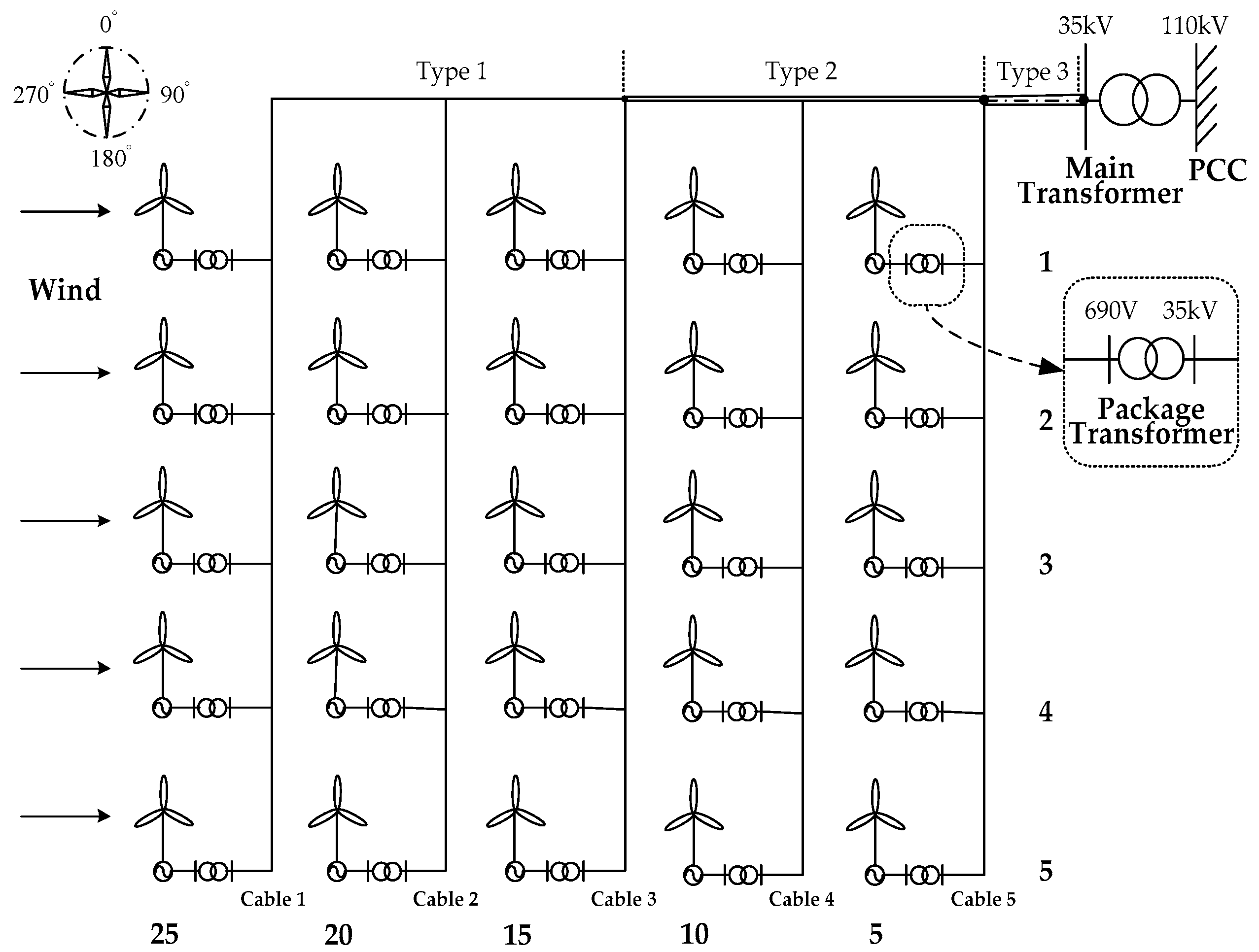
To verify the effectiveness of the proposed strategy, a simulation model based on the parameters of a large-scale WF is established using MATLAB/Simulink. This model has 25 5-MW turbines and the distance between the WTs is 882 m. The layout of the WF model is shown in Figure 6.
This WF model has three types of cables that are 95, 150, and 240 XLPE-Cu; the distribution of the cables is also shown in Figure 6. Appendix A describes the required parameters of the WT and the cables.
The structure of the WF model implemented in Simulink is shown in Figure 7. Five WTs on the same cable are packaged together and each WT is calculated independently. The outlet voltage of the WT is 690 V, the voltage on the high-voltage side of the package transformer is 35 kV, and the PCC is the bus with 110 kV.
4.2. Case 1: V = 9 m/s,
In this case, the wind velocity of the WF is assumed to be uniform because the wake effect is basically ignored by the distribution of the WTs in the current WF design. The two-parameter Weibull distribution of the wind source data is shown in Figure 8. In this case, 9 m/s is the highest input wind velocity and the reactive power demand of the PCC is 0.2 pu based on 125 MVA.
The traditional reactive power control of WFs is based on a proportional distribution and the total reactive power demand of the WF is evenly distributed based on the reactive power capacity of the WTs; it is calculated by Equation (21).
where is the reactive power instruction of WT i, is the reactive power capacity of WT i at this moment, is the total reactive power demand of the WF at this moment.
The reactive power dispatching instruction of the WTs for the proposed ORPD strategy optimized by the GA and PSO algorithm and the reactive power reference of the proportional dispatch are shown in Figure 9. It is observed that the reactive power reference is the same for each WT when the proportional dispatch strategy is used because the wind distribution in the WF is uniform. However, the reactive power reference in each cable has a downward trend when the proposed ORPD strategy optimized by the GA and PSO algorithm is used. If the WT is closer to the PCC in this WF, the connecting cable is much shorter and, as a result, the loss in the cable will be lower and the WT will obtain a higher reactive power reference in the proposed ORPD strategy.
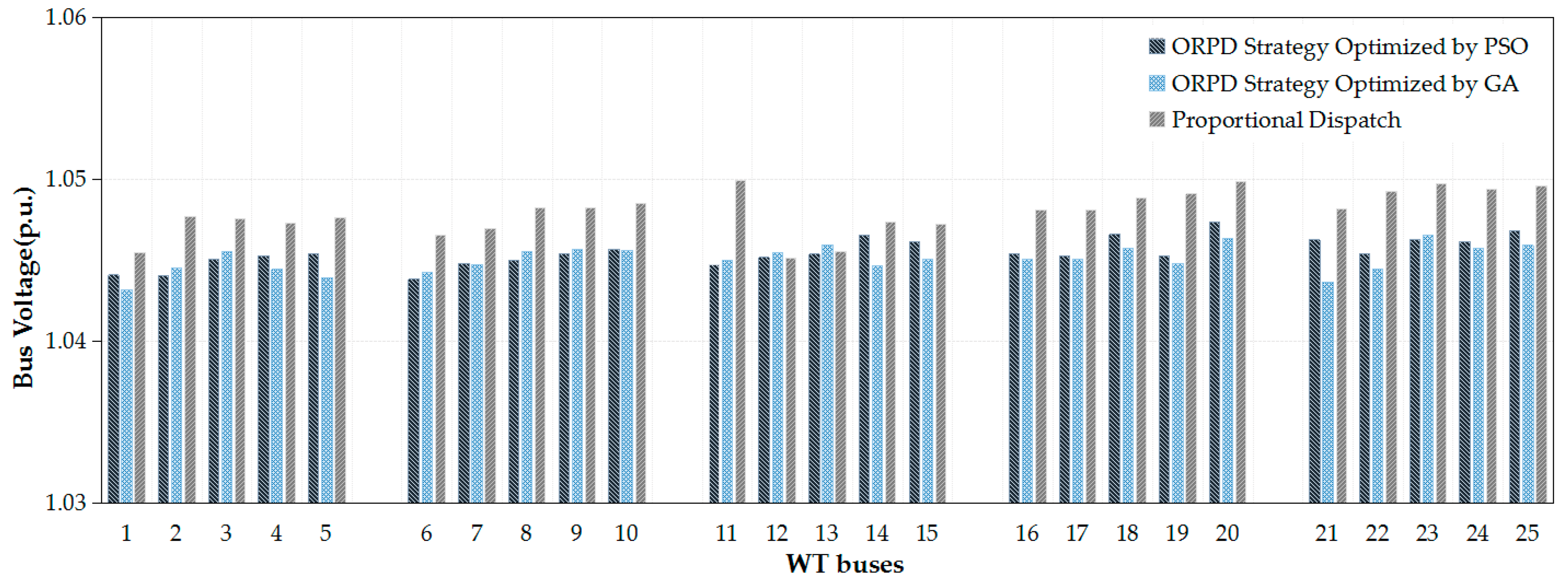
Meanwhile, the bus voltage at PCC optimized by GA is 1.0097 pu, the result optimized by PSO is 1.0098 pu and the result of traditional method is 1.01 pu. All of the WT bus voltages are shown in Figure 10. It can be seen that each voltage is within the constraints after optimization, moreover, the bus voltages optimized by GA and PSO maintain better balance and have greater stability margin.
In order to compare the effect of different reactive power dispatching strategies, the active power losses are recorded for each component of the collector system; the results are shown in Table 1 and Figure 11. It is clear that the reactive power optimization control reduces the loss in the collector circuit and the package transformers remarkably, whereas the main transformer is less affected.
The change in the solution space of the GA and PSO algorithm is shown in Figure 12, the initial populations are all randomly distributed, and the final solution space distributed differently. In the final solution space, all individuals in GA reach the same value, while only half of the PSO reach the optimal solution. However, both algorithms converge to the same solution, which represents the consistency of the optimization results. The convergence curves of the active power losses based on the GA and PSO algorithm are shown in Figure 13. The results show that there are no obvious differences in the optimization results for the GA and PSO algorithm, which illustrate the stability of the optimization strategy.
4.3. Case 2: V = 9 m/s,
The total losses of the active power for different dispatching methods and for values of ranging from −0.2 pu to 0.2 pu are shown in Figure 14. It is evident that the reactive power optimization control strategy reduces the active power loss of the WF effectively under the different reactive power demands of the PCC. The optimization results are better for the GA than the PSO algorithm at and .
4.4. Total Annual Losses in the WF
Since the total losses of the WF vary with wind speed, it is essential to verify the effectiveness of the proposed strategy by calculating the annual losses of the WF and to further compare the performance of the GA and PSO algorithm for addressing the reactive power optimal control problem. Based on the annual wind resources (Figure 7) and assuming the normal operation of the WTs, the estimated annual power generation of the WF under different reactive power demands of the PCC is in the range of 448 GWh to 453 GWh.
The calculation results are shown in Table 2. It is evident that the results optimized by the GA and PSO are much better than the proportional dispatch method under different reactive power requirements of the PCC. Moreover, the difference between the GA and PSO is in the range of 0.03 GWh to 0.05 GWh and the energy savings are little better when the GA is used for the optimization.
4.5. Environmental Indicators Analysis
We also calculated the reductions in the standard coal consumption and the carbon and CO2 emissions as suggested in reference [22]. We use the ORPD strategy optimized by the GA as an example and the annual WF loss reduction shown in Table 2. The results in Table 3 show the annual reductions in the standard coal consumption and the reductions in CO2 and carbon emissions. It can be observed that, compared with the proportional dispatch strategy, the proposed ORPD strategy saves up to 308 tons of standard coal every year, which is equivalent to cutting 604.45 tons of CO2 emissions and 209.44 tons of carbon emissions when the reference of the reactive power at the PCC is −0.2 pu.
5. Conclusions
In this paper, we proposed a reactive power control strategy for WFs aimed at energy savings. A reactive power optimization model is established and simulation experiments are conducted under several working conditions. The following conclusions are drawn based on the results:
- Combining the reactive power/voltage control with the loss reduction control of the collector system reduces the operating loss of the WF effectively; this is verified by a simulation based on an actual wind farm.
- Both the GA and PSO optimization methods designed in this paper can reduce the operating loss effectively but the GA has a better performance of energy savings with regard to the annual loss in this case.
- The control strategy proposed in this paper would be used to improve the automatic control level, reduce the cost of electricity production, and improve the energy savings under various operating conditions of a WF, which has good application prospects.
Author Contributions
Conceptualization, Y.X.; Methodology, Y.X. and Y.W.; Software, Y.W.; Validation, Y.X.; Formal Analysis, Y.X.; Resources, Y.S.; Data Curation, Y.S.; Writing-Original Draft Preparation, Y.W.; Writing-Review & Editing, Y.X.; Project Administration, Y.S.; Funding Acquisition, Y.X.
Acknowledgments
This research work is supported by the Fundamental Research Funds for the Central Universities of China (2018MS27), and the National Natural Science Foundation of China (51677067). The authors are grateful for the support. In addition, the authors would like to thank North China Electric Power Research Institute Co. for providing the wind farm data and application support.
Conflicts of Interest
The authors declare no conflict of interest.
Appendix A
The parameters of 5 MW WT used in this paper are shown in Table A1.

Table A1.
5-MW wind turbine specifications.
| Parameter | 5 MW NERL Wind Turbine |
|---|---|
| Cut-in, Rated, Cut-out Wind Velocity | 3 m/s, 11.4 m/s, 25 m/s |
| Rotor, Hub Diameter | 126 m, 3 m |
| Rated Power | 5 MW |
| Cut-in, Rated Rotor Velocity | 6.9 rpm, 12.1 rpm |
| Gearbox Ratio | 97:1 |
The cable parameters of the collector system in the WF model are shown in Table A2.
Table A2.
Network Parameters.
| Cable Types | Cross Section (mm2) | Specific Resistance (Ω/km) | Specific Capacitance (μF/km) | Specific Inductance (μH/km) |
|---|---|---|---|---|
| Type 1 | 95 | 0.1842 | 0.18 | 0.44 |
| Type 2 | 150 | 0.1167 | 0.21 | 0.41 |
| Type 3 | 240 | 0.0729 | 0.24 | 0.38 |
References
- National Grid plc. The Grid Code (Issue 5, Revision 13). Available online: http://www.nationalgrid.com/uk (accessed on 2 June 2018).
- Qiao, W.; Harley, R.G.; Venayagamoorthy, G.K. Coordinated reactive power control of a large wind farm and a STATCOM using heuristic dynamic programming. IEEE Trans. Energy Convers. 2009, 24, 493–503. [Google Scholar] [CrossRef]
- El Moursi, M.S.; Bak-Jensen, B.; Abdel-Rahman, M.H. Coordinated voltage control scheme for SEIG-based wind park utilizing substation STATCOM and ULTC transformer. IEEE Trans. Sustain. Energy 2011, 2, 246–255. [Google Scholar] [CrossRef]
- Kumar, V.S.S.; Reddy, K.K.; Thukaram, D. Coordination of reactive power in grid-connected wind farms for voltage stability enhancement. IEEE Trans. Power Syst. 2014, 29, 2381–2390. [Google Scholar] [CrossRef]
- Khatua, K; Yadav, N. Voltage stability enhancement using VSC-OPF including wind farms based on Genetic algorithm. Int. J. Electr. Power Energy Syst. 2015, 73, 560–567. [Google Scholar] [CrossRef]
- Guo, W.T.; Liu, F.; Si, J.N.; He, D.W.; Harley, R.; Mei, S.W. Approximate dynamic programming based supplementary reactive power control for DFIG wind farm to enhance power system stability. Neurocomputing 2015, 170, 417–427. [Google Scholar] [CrossRef]
- Ni, K.; Hu, Y.H.; Liu, Y.; Gan, C. Performance analysis of a four-switch three-phase grid-side converter with modulation simplification in a doubly-fed induction generator-based wind turbine (DFIG-WT) with different external disturbances. Energies 2017, 10, 706. [Google Scholar] [CrossRef]
- Jung, S.; Jang, G. A loss minimization method on a reactive power supply process for wind farm. IEEE Trans. Power Syst. 2017, 32, 3060–3068. [Google Scholar] [CrossRef]
- Wijethunga, A.H.; Ekanayake, J.B.; Wijayakulasooriya, J.V. Collector cable design based on dynamic line rating for wind energy applications. J. Natl Sci. Found. Sri Lanka 2018, 46, 31–40. [Google Scholar] [CrossRef]
- Gong, Y.Z.; Chung, C.Y.; Mall, R.S. Power system operational adequacy evaluation with wind power ramp limits. IEEE Trans. Power Syst. 2018, 33, 2706–2716. [Google Scholar] [CrossRef]
- Wang, D.; Hu, Q.E.; Tang, J.; Jia, H.J.; Li, Y.; Gao, S.; Fan, M.H. A kriging model based optimization of active distribution networks considering loss reduction and voltage profile improvement. Energies 2017, 10, 2162. [Google Scholar] [CrossRef]
- Guo, Q.L.; Sun, H.B.; Wang, B.; Zhang, B.M.; Wu, W.C.; Tang, L. Hierarchical automatic voltage control for integration of large-scale wind power: Design and implementation. Electr. Power Syst. Res. 2015, 120, 234–241. [Google Scholar] [CrossRef]
- Adebayo, I.; Sun, Y.X. New performance indices for voltage stability analysis in a power system. Energies 2017, 10, 2042. [Google Scholar] [CrossRef]
- Wei, S.R.; Zhang, L.; Xu, Y.; Fu, Y.; Li, F.X. Hierarchical optimization for the double-sided ring structure of the collector system planning of large offshore wind farms. IEEE Trans. Sustain. Energy 2017, 8, 1029–1039. [Google Scholar] [CrossRef]
- Zhang, B.H.; Hou, P.; Hu, W.H.; Soltani, M.; Chen, C.; Chen, Z. A reactive power dispatch strategy with loss minimization for a DFIG-based wind farm. IEEE Trans. Sustain. Energy 2016, 7, 914–923. [Google Scholar] [CrossRef]
- Meegahapola, L.; Durairaj, S.; Flynn, D.; Fox, B. Coordinated utilisation of wind farm reactive power capability for system loss optimisation. Int. Trans. Electr. Energy Syst. 2011, 21, 40–51. [Google Scholar] [CrossRef]
- Abdelsalam, A.M.; El-Shorbagy, M.A. Optimization of wind turbines siting in a wind farm using genetic algorithm based local search. Renew. Energy 2018, 123, 748–755. [Google Scholar] [CrossRef]
- Devaraj, D.; Roselyn, J.P. Genetic algorithm based reactive power dispatch for voltage stability improvement. Int. J. Electr. Power Energy Syst. 2010, 32, 1151–1156. [Google Scholar] [CrossRef]
- Amini, M.H.; Moghaddam, M.P.; Karabasoglu, O. Simultaneous allocation of electric vehicles’ parking lots and distributed renewable resources in smart power distribution networks. Sustain. Cities Soc. 2017, 28, 332–342. [Google Scholar] [CrossRef]
- Tahir, M.; Nassar, M.E.; El-Shatshat, R.; Salama, M.M.A. A review of volt/var control techniques in passive and active power distribution networks. IEEE Smart Energy Grid Eng. 2016, 57–63. [Google Scholar] [CrossRef]
- Han, X.J.; Zhang, H.; Yu, X.L.; Wang, L.N. Economic evaluation of grid-connected micro-grid system with photovoltaic and energy storage under different investment and financing models. Appl. Energy 2016, 184, 103–118. [Google Scholar] [CrossRef]
- Yu, S.W.; Zhang, J.J.; Cheng, J.H. Carbon reduction cost estimating of Chinese coal-fired power generation units: A perspective from national energy consumption standard. J. Clean. Prod. 2016, 139, 612–621. [Google Scholar] [CrossRef]
Figure 1.
Proposed reactive power control system.
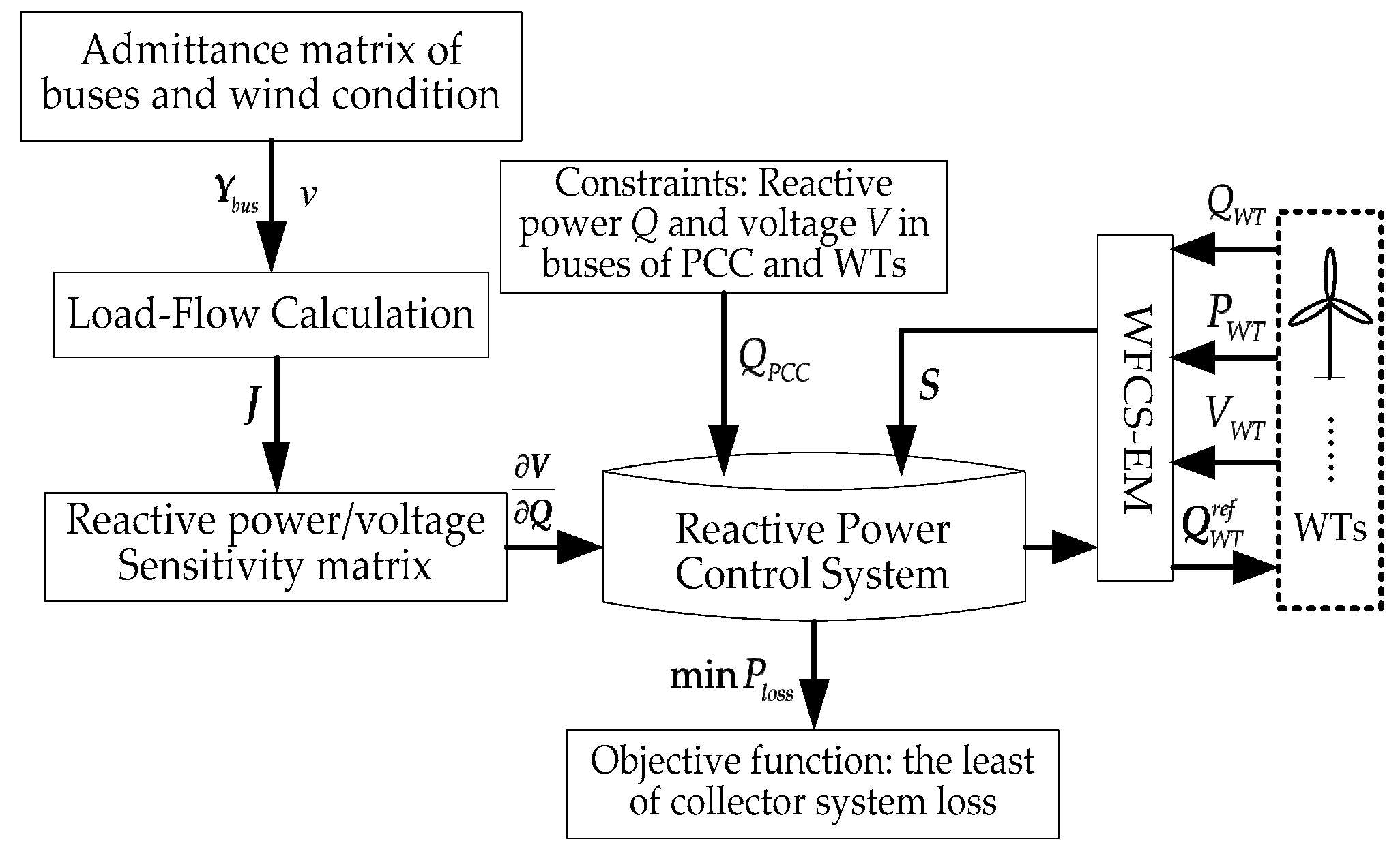
Figure 2.
Flowchart of the dynamic reactive power control system.
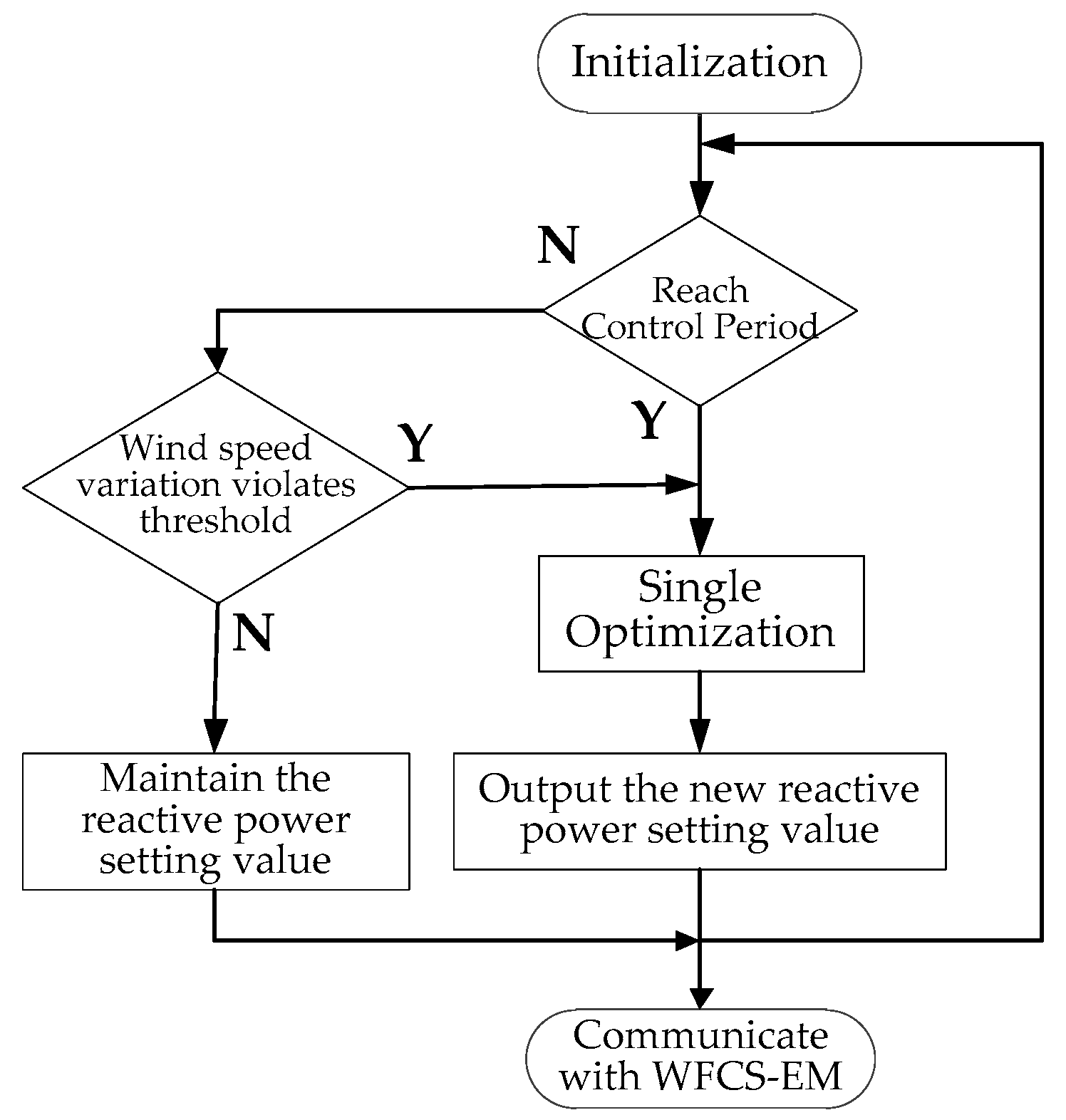
Figure 3.
Schematic of collector cables.

Figure 4.
Basic structure of a Genetic Algorithm (GA).

Figure 5.
Basic structure of the particle swarm optimization (PSO) algorithm.

Figure 6.
Layout of the wind farm (WF) model.

Figure 7.
A screenshot of the WF structure in the simulation.
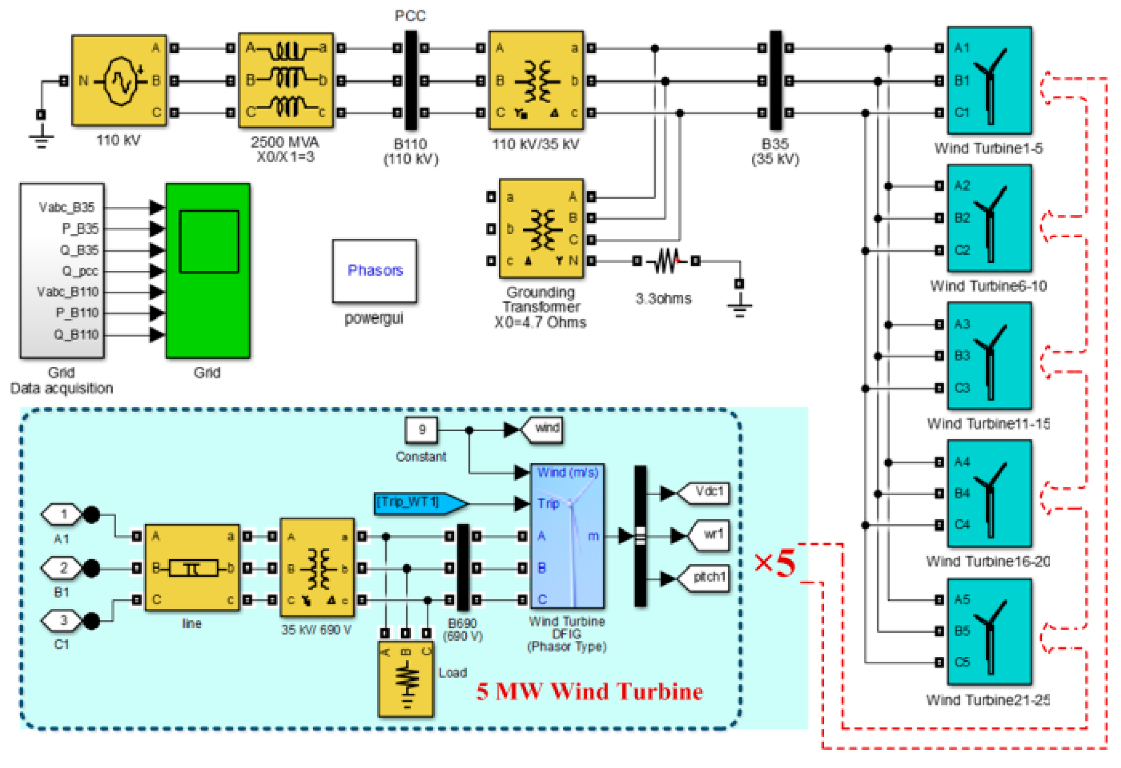
Figure 8.
Frequency distribution of the wind velocity.

Figure 9.
Distributed reactive power in WF when required reactive power references at the point of common coupling (PCC) are set to 0.2 pu.
Figure 9.
Distributed reactive power in WF when required reactive power references at the point of common coupling (PCC) are set to 0.2 pu.

Figure 10.
Wind turbine (WT) bus voltage when required reactive power references at PCC are set to 0.2 pu.
Figure 10.
Wind turbine (WT) bus voltage when required reactive power references at PCC are set to 0.2 pu.

Figure 11.
Losses in the WF using different dispatch strategies.

Figure 12.
Convergence trend of the algorithms. (a) The initial solution space of the GA and PSO algorithm; (b) The final solution space of the GA and PSO algorithm.
Figure 12.
Convergence trend of the algorithms. (a) The initial solution space of the GA and PSO algorithm; (b) The final solution space of the GA and PSO algorithm.
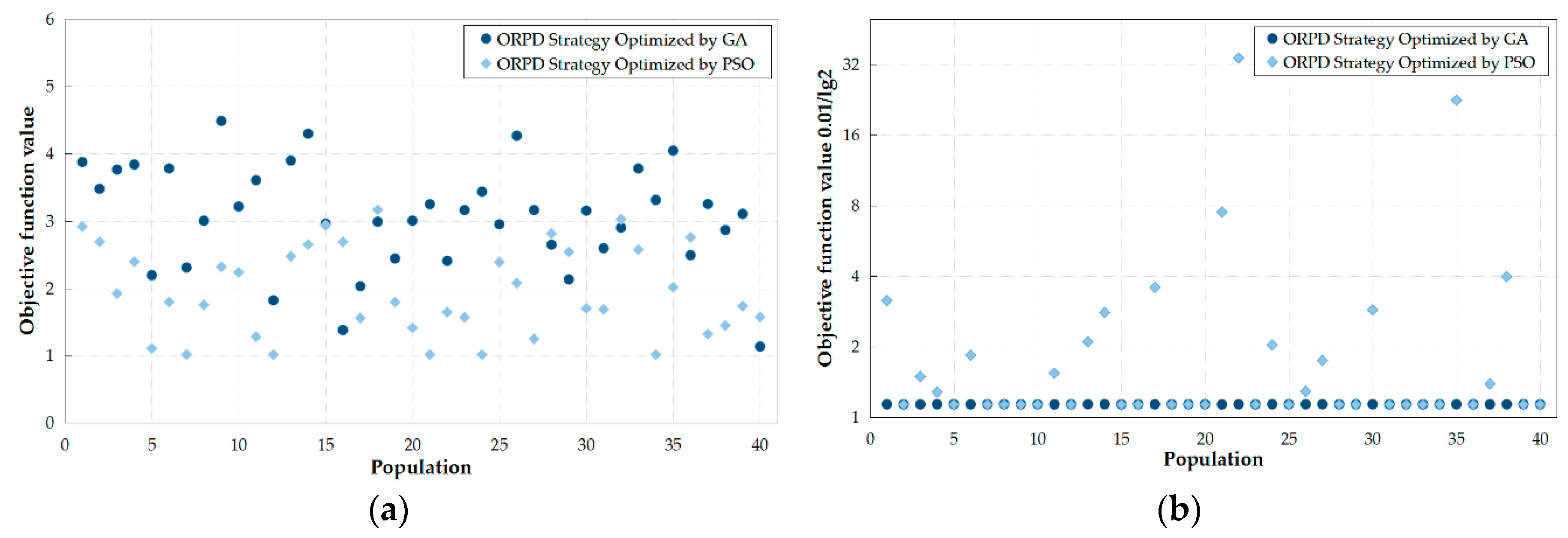
Figure 13.
Changes in the active power loss versus the number of iterations for the different algorithms.
Figure 13.
Changes in the active power loss versus the number of iterations for the different algorithms.
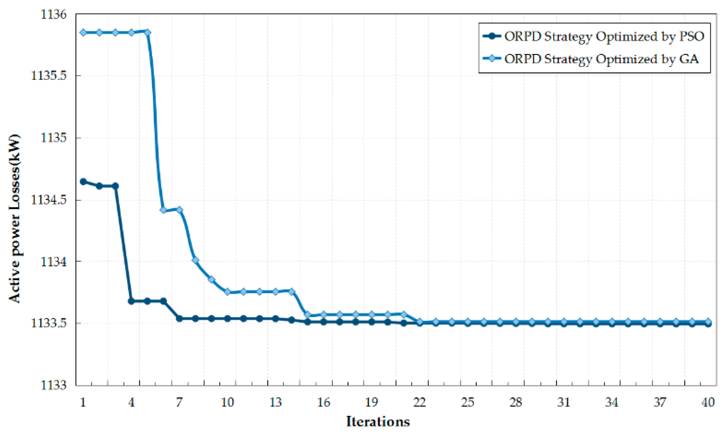
Figure 14.
Total loss curves of the optimal reactive power dispatch (ORPD) strategy and proportional dispatch as the reference reactive power changes at the PCC.
Figure 14.
Total loss curves of the optimal reactive power dispatch (ORPD) strategy and proportional dispatch as the reference reactive power changes at the PCC.
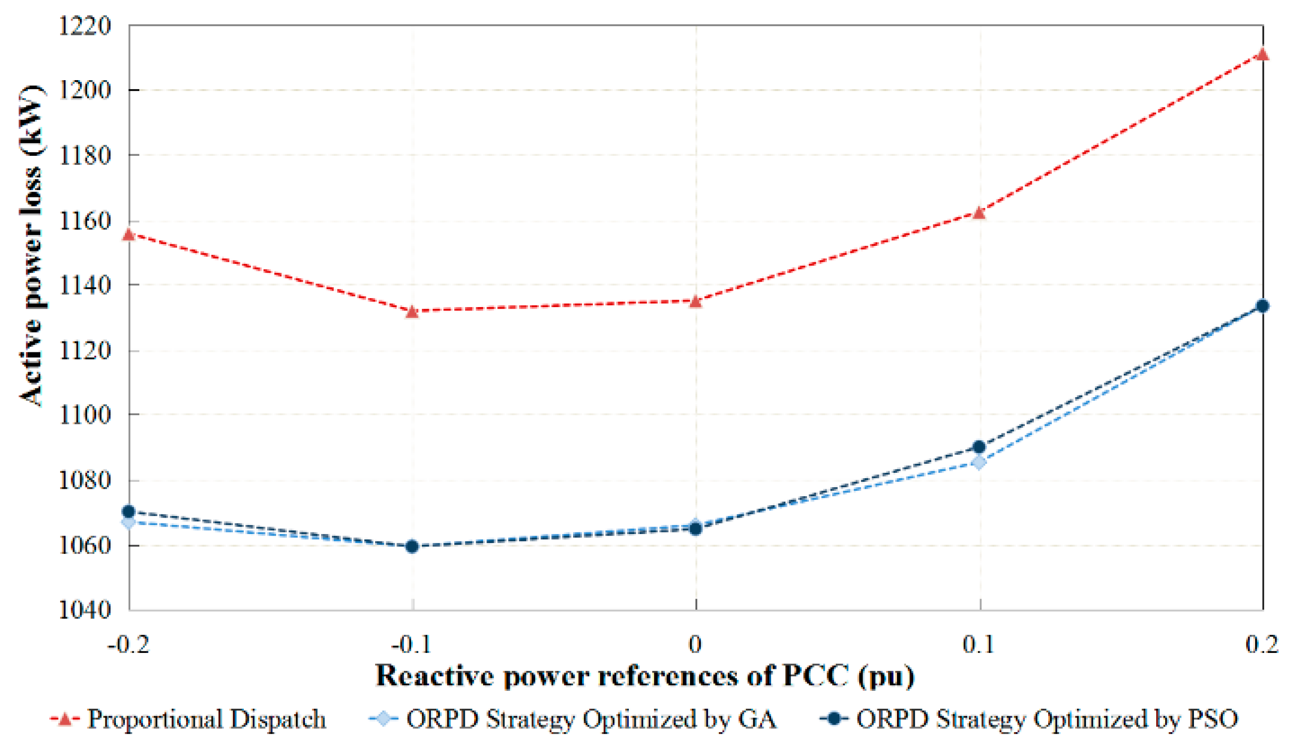
Table 1.
Losses in the WF using different dispatching strategies.
| Strategy of Dispatch | Proportional Dispatch | ORPD Strategy | ||
|---|---|---|---|---|
| WF Loss (kW) | Optimized by GA | Optimized by PSO | ||
| Cable + Package Transformers | 529.03 | 452.44 | 452.35 | |
| Main Transformer | 682.30 | 681.15 | 681.15 | |
| Total | 1211.34 | 1133.59 | 1133.49 | |
Table 2.
Total annual losses.
| Proportional Dispatch (GWh) | Proportion of Losses | ORPD Strategy | ||||
|---|---|---|---|---|---|---|
| GA (GWh) | Proportion of Losses | PSO (GWh) | Proportion of Losses | |||
| −0.2 | 9.57 | 2.12% | 8.81 | 1.94% | 8.86 | 1.96% |
| −0.1 | 9.37 | 2.07% | 8.7 | 1.92% | 8.74 | 1.93% |
| 0 | 9.37 | 2.07% | 8.74 | 1.93% | 8.77 | 1.93% |
| 0.1 | 9.58 | 2.12% | 8.91 | 1.97% | 8.94 | 1.97% |
| 0.2 | 9.9 | 2.21% | 9.18 | 2.04% | 9.22 | 2.06% |
Table 3.
Reductions in standard coal consumption and carbon emissions.
| Annual Loss Reduction (GWh) | Standard Coal (t/year) | CO2 Emissions (t/year) | Carbon Emissions (t/year) | |
|---|---|---|---|---|
| −0.2 | 0.77 | 308 | 604.45 | 209.44 |
| −0.1 | 0.67 | 272 | 533.8 | 182.24 |
| 0 | 0.63 | 256 | 502.4 | 171.36 |
| 0.1 | 0.66 | 268 | 525.95 | 179.52 |
| 0.2 | 0.73 | 284 | 557.35 | 198.56 |
© 2018 by the authors. Licensee MDPI, Basel, Switzerland. This article is an open access article distributed under the terms and conditions of the Creative Commons Attribution (CC BY) license (http://creativecommons.org/licenses/by/4.0/).
Share and Cite
MDPI and ACS Style
Xiao, Y.; Wang, Y.; Sun, Y. Reactive Power Optimal Control of a Wind Farm for Minimizing Collector System Losses. Energies 2018, 11, 3177. https://doi.org/10.3390/en11113177
AMA Style
Xiao Y, Wang Y, Sun Y. Reactive Power Optimal Control of a Wind Farm for Minimizing Collector System Losses. Energies. 2018; 11(11):3177. https://doi.org/10.3390/en11113177
Chicago/Turabian StyleXiao, Yunqi, Yi Wang, and Yanping Sun. 2018. "Reactive Power Optimal Control of a Wind Farm for Minimizing Collector System Losses" Energies 11, no. 11: 3177. https://doi.org/10.3390/en11113177
Note that from the first issue of 2016, this journal uses article numbers instead of page numbers. See further details here.