Hardware in the Loop Real-Time Simulation for Heating Systems: Model Validation and Dynamics Analysis

Abstract

Heating systems such as heat pumps and combined heat and power cycle systems (CHP) represent a key component in the future smart grid. Their capability to couple the electricity and heat sector promises a massive contribution to the energy transition. Hence, these systems are continuously studied numerically and experimentally to quantify their potential and develop optimal control methods. Although numerical simulations provide time and cost-effective solutions for system development and optimization, they are exposed to several uncertainties. Hardware in the loop (HiL) approaches enable system validation and evaluation under different real-life dynamic constraints and boundary conditions. In this paper, a HiL system of a heat pump testbed is presented. It is used to present two case studies. In the first case, the conventional heat pump testbed operation method is compared to the HiL operation method. Energetic and dynamic analyses are performed to quantify the added value of the HiL and its necessity for dynamics analysis. In the second case, the HiL testbed is used to validate a model of a single family house with a heat pump participating in a local energy market. The energetic analysis indicates a deviation of 2% and 5% for heat generation and electricity consumption of the heat pump model, respectively. The model dynamics emphasized its capability to present the dynamics of a real system with a temporal distortion of 3%.

1. Introduction

Installed renewable energy capacities are growing fast worldwide. At the end of 2017, 2179 GW were installed, with a growth rate of 8.3% [1,2]. These capacities are expected to continue growing to minimize the CO${}_2$ emissions and mitigate the climate change. In Germany, several legislations were introduced to create a nuclear and fossil-free economy within the framework of the energy transition [3]. Among these acts are the renewable energy act, Erneuerbare Energien Gesetz (EEG), and the combined heat and power act, Kraft-Wärme-Kopplungsgesetz (KWKG). The EEG prioritizes the renewable energy sources (RES) in the energy market [4]. It guarantees a fixed feed-in tariff for the supplier to minimize the risk of the investors. Hence, the RES reached 111 GW in 2017 [4]. On the other hand, KWKG empowers the integration of combined heat and power (CHP) systems in the national grid. A goal was set to generate 25% of the electricity by co-generation by 2020 [5]. As these two acts increased the renewable energy capacities and increased the system efficiency, they raised several challenges in the national grid and made the traditional grid management techniques rather obsolete.

Sector coupling is one way to address these challenges faced by the grid. Heat pumps and CHP systems are the key drivers behind the electricity and heat sectors coupling. The attractive costs and lifespan of heat storages enable these heating systems to be the most economically feasible candidates to offer flexibility and mitigate the fluctuating RES. Moreover, the continuous improvement of these systems efficiency led to a significant decrease in the operation and maintenance costs [6].

Given these heating systems potential in the current and future national energy system, several researchers modeled and studied these heating systems [7,8,9,10,11,12,13]. Although the presented heating system models can predict to a reasonable extent the energy generation or consumption of a real-system, they are exposed to several uncertainties as they are designed to be integrated into larger models under specific system constraints. Hence, field tests and testbeds were used to investigate the quality of the results and analyze the real-life system dynamics. Although field tests provided the utmost accurate results, they are costly and do not offer enough control flexibility [8]. For control algorithms’ development and evaluation, testbeds are considered the most feasible option [14,15]. However, the testbed operation approach can significantly influence the results.

Hardware in the loop (HiL) is an approach to simulate and evaluate thermal system dynamics under multiple environmental constraints. The fundamental idea of the HiL is to integrate real hardware in a simulation loop. Real hardware replaces the numerical model of a system to study and evaluate the quality of a developed control or optimization algorithm [16]. Hardware can also be integrated with multiple numerical models to investigate its reaction to different model combinations. As an example, a HiL system of a heat pump as hardware and a controller as software can be used to evaluate the quality of the control system. Also, a building model can be integrated to show the heat pump dynamics and reaction to different building types, ages or sizes.

In the literature, HiL simulation is being used in several fields. According to [16,17], it has been used for over 50 years. An early application was in the flight and missiles control industry as in the Sidewinder program in 1972 [18]. It has also become more popular in other industries. As an example, HiL represents a crucial tool in the automotive industry nowadays [17,19]. It is extensively used for engine and suspension systems control and design. Moreover, Hil is also used for testing unmanned aerial vehicles as in [20]. In the electrical power sector, applications of HiL for testing and validating are growing. Sun et al. [21] used a HiL system to study the dynamic performance of a switch-mode power amplifier. In [22] a power HiL system was introduced and used to evaluate a case study of a Great Britain network. Rosa et al. [23] implemented a HiL system to investigate and compare the performance of multiple control techniques for Single-Ended Primary Inductance Converter (SEPIC). Castaings et al. [24] investigated different energy management strategies with electric vehicles using a HiL system in real-time. The author’s setup facilitated the evaluation of the effectiveness of the designed EMS strategies in real-time. Furthermore, Ruuskanen et al. [25] designed a HiL system for water electrolysis system emulation. Through this system, the author was able to study the electrolyzer characteristics in a smart grid. In [26], voltage control coordination scenarios were validated based on a HiL system. The authors used HiL in a real-time simulation to validate the capability of RES to provide voltage control in a smart grid.

Although several publications are available for power HiL systems, a limited number of publications discussed the heating systems in buildings. Among these publications is the work of [27], where a HiL simulation system was developed to evaluate the control strategies of a hydronic radiant heating system. The author replaced the model of a hydronic network with real hardware to minimize the results uncertainties. In [28], a HiL system was developed to simulate micro-CHP systems with different building models. The author showed the necessity of a HiL system in the operation of micro-CHP testbeds and evaluation of optimization and control algorithms.

At the Institute of energy economy and application technology (IfE), several testbeds were developed to evaluate the common heating systems at different scales as in [14,29,30] and recently in [15]. A testbed is necessary to demonstrate and validate the novel optimization algorithms and control strategies being developed. Through these testbeds, the operational requirements and technical constraints were easily defined. Ideally, a heating system testbed should also be able to demonstrate and emulate a real building with a heating system and is expected to eliminate all the uncertainties, as real hardware is used. However, as the buildings are emulated by heat sinks, uncertainties can emerge, and the building dynamics in certain cases diminish. Thus, a HiL system was introduced in [28] to address these uncertainties with micro-CHPs operation. In this paper, the recent advanced HiL version of [28], the testbed in [15] and model presented in [31] are used to demonstrate the following aspects:

• A comparison between heating systems testbeds operation with HiL and without HiL system simulation
• An energetic and dynamics analysis to quantify the benefits of HiL simulation with heating systems
• A model validation of the heat pump dynamics and interactions within a microgrid

The structure of the paper is as follows. Section 2 shortly describes the different numerical and experimental methods used to analyze a heating system. Section 3 demonstrates the HiL system structure including the testbed and building model. Moreover, it presents the input system parameters. Section 4 demonstrates the results of the two different case studies. Section 5 presents a conclusive summary.

2. Heating Systems Analysis Methods

Numerical simulation provides the ideal environment for testing and evaluation of a heating system performance connected to different buildings types. Compared to experimental testing, it saves efforts, costs, and time to investigate a specific heating system. However, it is exposed to several uncertainties, and its accuracy is questionable. Hence, the experimental investigation has always an edge over the numerical simulation as it eliminates the modeling uncertainties.

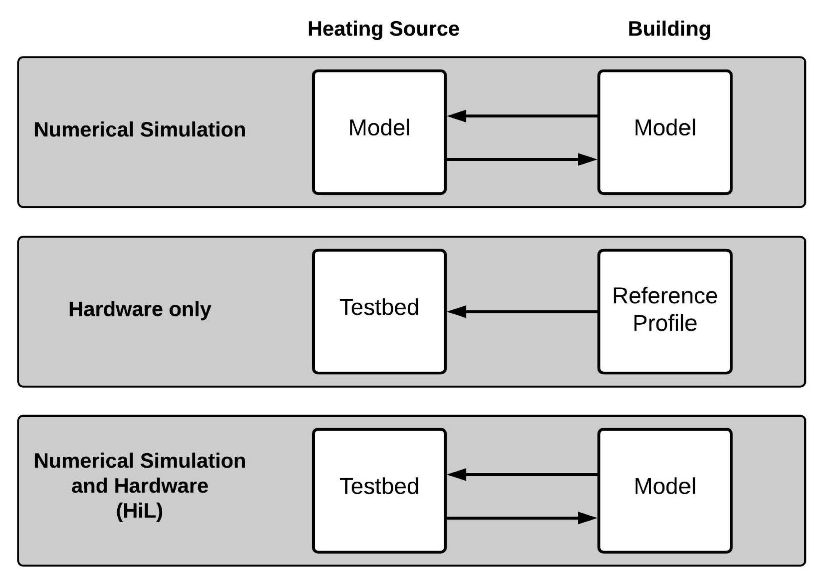
The experimental testing can only be performed using hardware, or hardware and numerical models as HiL. Figure 1 presents an abstract comparison between heating system analysis using numerical simulation, hardware only (without HiL), and hardware and numerical models (HiL). The conventional method to evaluate the heating system experimentally is using hardware only. A reference profile that is obtained within a field test or by a simulation model is fed directly to the testbed. This reference profile contains the thermal load of the building over a specific period of time. The testbed hydraulic circuit emulates this load profile using a heat sink to evaluate the reaction of the heat source and heat storage. Although the heating source such as a heat pump or a micro-CHP system is a real system, the results of the whole experiment are exposed to uncertainties because of the heat sink emulation of the reference load profile. The heat sink always tries to reach the set reference profile, even if it has to decrease the return temperature to or below the room temperature. As a conventional alternative solution, return temperature can be held constant, yet it diminishes the dynamics of the whole testbed operation.

A combination of hardware and numerical simulation is considered to be the optimal method for heating systems analysis and models validation. The heat source and heat storage are integrated as hardware with a building model using HiL system to evaluate and validate heating systems dynamics and performance. Consequently, the building model can calculate realistic return temperatures and the feedback of the building for any violations introduced by the heating source. Furthermore, the room temperature can be simulated by the building model to analyze the user comfort in real-time.

3. HiL Simulation System

3.1. Communication Structure

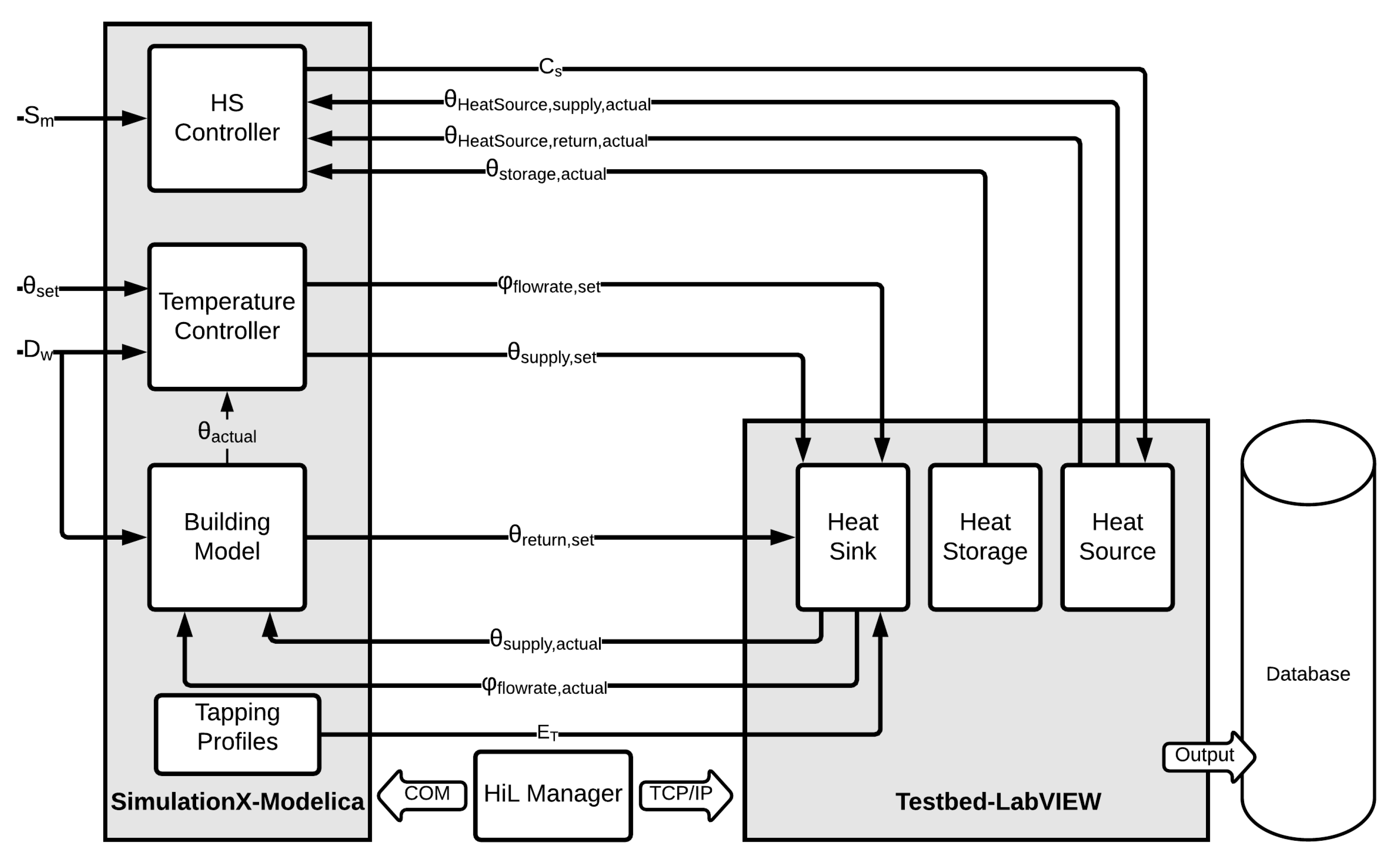
Figure 2 shows the detailed control loop of the implemented HiL model. The heat pump (HP) controller, temperature controller, building model, and the tapping profiles are implemented in SimulationX, which is a Modelica based software. More details about the models are explained later in this section. The testbed, the hardware, is presented by three modules: heat sink, heat storage, and heat source, which are the typical components of a heating system testbed. A LabVIEW program controls the different components of the testbed and feeds the output to the database.

The communication between the model in SimulationX and LabVIEW is managed by the HiL manager, which is based on MATLAB. The data is transferred using the TCP/IP protocol between the HiL manager and LabVIEW, while COM interface is used to manage the SimulationX. The details of the HiL manager communication protocols and sequence are thoroughly documented in [28].

Other communication systems were tested such as exporting the building models in the C programming language (C-code) and importing the model in LabVIEW. However, processing the C-code in real-time desynchronizes the LabVIEW real-time control loop. Moreover, the number of inputs and outputs to and from the C-code are limited. Hence, using C-code for integrating models in real-time LabVIEW control systems is not feasible for heating systems applications.

The communicated data between the testbed and the SimulationX models is dependent on the functionality of the model and testbed module. The HS controller receives the actual heat source supply temperature ${\theta }_{HeatSoruce,supply,actual}$, actual heat source return temperature ${\theta }_{HeatSoruce,return,actual}$, and temperature of the storage ${\theta }_{storage,actual}$ from the testbed. Moreover, it receives an external control input signal $S_m$ that is developed from the model described in [31]. Based on these input signals, the HS controller sends a binary operation signal $C_s$ to the testbed heat source. The temperature controller receives ${\theta }_{set}$ and ${\theta }_{actual}$, which are the set room temperature and the actual room temperature, respectively. Based on these two inputs and weather data $D_w$, the temperature controller can calculate the set flow rate ${\phi }_{flowrate,set}$, and the set space heating supply temperature of the ${\theta }_{supply,set}$. The building model receives $D_w$, actual flow rate ${\phi }_{flowrate,actual}$, and the actual supply temperature of the space heating ${\theta }_{supply,actual}$. Based on these inputs and the building model, the return temperature ${\theta }_{return,set}$ can be calculated and forwarded to the testbed. Communicating the ${\theta }_{return,set}$ each second in this HiL simulation system maximizes the results accuracy and enables the testbeds to present realistic dynamics that is comparable to field measurements. Tapping profiles can also be integrated as a model and communicated as energy profiles $E_T$ to the heat sink.

3.2. Testbed Components and Description

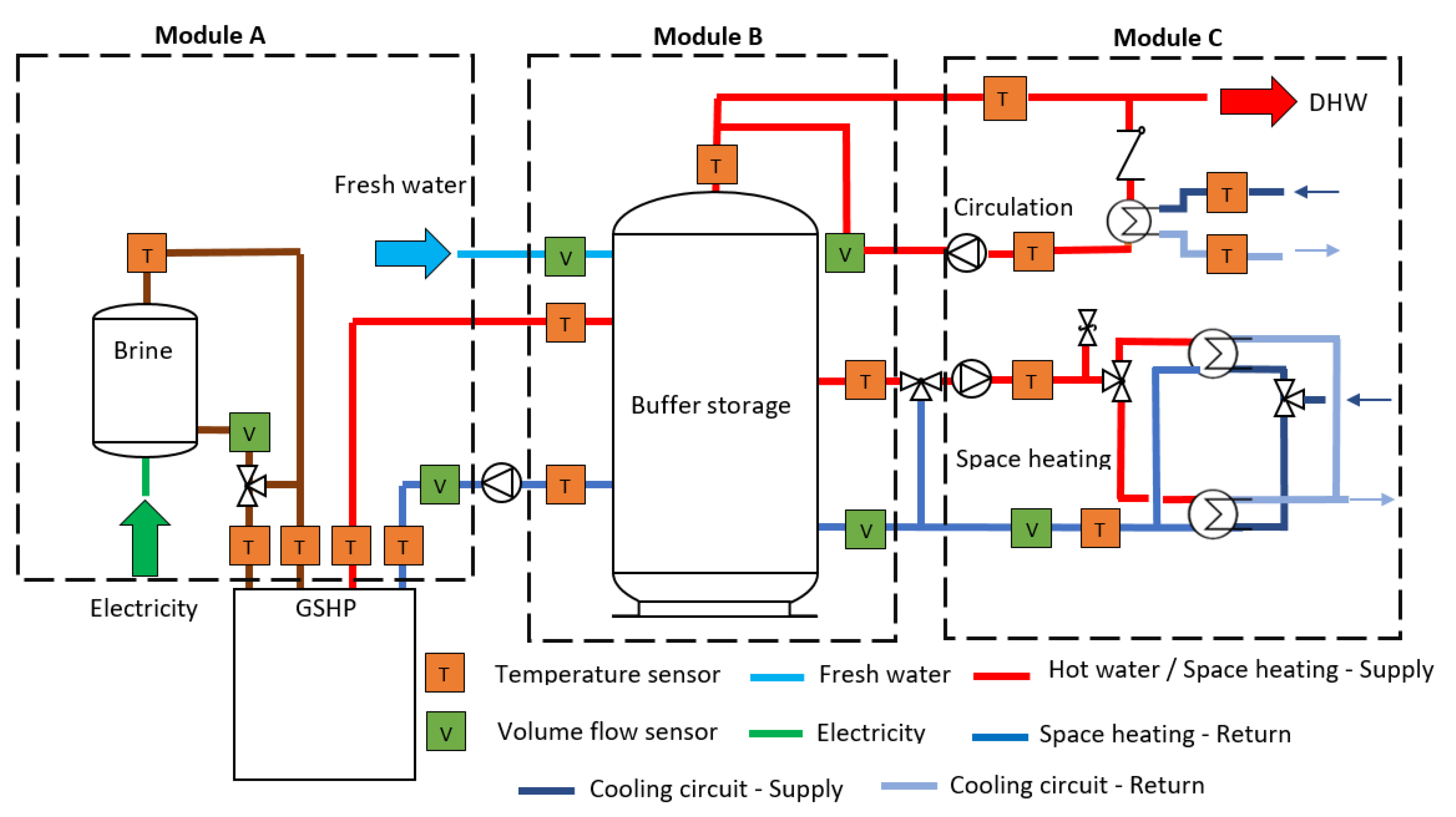
The testbed system consists of three modules and a brine water heat pump with a thermal power of 10.31 kW and a COP of 5.02 by B0/W35 as per standard EN14511. Two circulations pumps are integrated into the heat pump on the brine and the water side. Moreover, it is equipped with an emergency electrical heater of 8.8 kW. Figure 3 shows the simplified hydraulic schematic of the used testbed.

A ground-source heat pump required an emulator to show the dynamics of the ground heat exchanger. Module A includes a ground-source emulator that can provide any required brine temperature to the heat pump. It consists of 300 L heat storage, filled with a water-glycol mixture as an anti-freezing heat transfer fluid. The storage is heated by a 12.5 kW electrical heater that is controlled via a hysteresis regulator to maintain the tank temperature during the whole operation time at 40 °C. The set temperature of the tank and the hysteresis bandwidth can be defined by the user depending on the simulation goals. A mixer, similar to the conventional space heating mixers, is used to mix the supply of brine tank with the return of the heat pump to reach the required ground-source set temperature. Depending on the HiL system and the goal of the simulation, the mixer can maintain a constant brine temperature or a time-dependent temperature profile.

Module B shows the combi-storage system of a conventional residential house. It includes a 749 L combi hygienic buffer storage to cover the space heating and domestic hot water consumption. A stainless steel heat exchanger extracts heat from the storage to cover the hot water consumption. Moreover, a coaxial pipe, pipe-in-pipe system, is used to enable the hot water circulation and maintain the pipe temperatures at a certain level.

Module C is the most complex module as it represents the heat sink of the testbed. It can emulate the space heating and domestic hot water consumption depending on the building type and user behavior. The space heating circuit consists of a space heating mixer, circulation pump, and two heat exchangers. Through the mixer, the supply of the tank with the return of the space heating is mixed to reach the required ${\theta }_{supply,set}$. The circulation pump is controlled according to ${\phi }_{flowrate,set}$, which varies depending on the heat demand. Two heat exchangers of two different sizes are used to emulate different building loads depending on their required maximum heat power. The domestic hot water consumption is emulated through three magnetic valves that have different consumption flow rates. These valves can represent different consumption activities such as washing, showering or cooking.

The hydraulic configuration in Figure 3 shows only one of the most common hydraulic configurations. However, the testbed can allow several other configurations, such as a direct connection of the heat pump to module C or using additional heat storage for hot water consumption. More details about the hydraulics, control, and dynamics of the testbed are available in [15].

3.3. Models Description

Earlier in [31], a market model is presented based on a double-sided auction, in which different household devices and heating systems can participate. The heating system bids their energy needs to either decrease costs or increase comfort. In this paper, the market control approach is going to be used to develop the external control signal, $S_m$. The control signal provided in this case is a binary signal, either 0 or 1. The HS controller reacts to the signal as in Equation (1), where ${\theta }_{HeatSource,supply,max}$ is the maximum heat source supply temperature, ${\theta }_{HeatSource,return,max}$ is the maximum heat source return temperature, and ${\theta }_{storage,max}$ is the maximum storage temperature at a specified sensor position.

$$C_S=\left\{\begin{array}{ll}0,& \mathrm{if}{\theta }_{HeatSource,supply,actual}\ge {\theta }_{HeatSource,supply,max},\\ 0,& \mathrm{if}{\theta }_{HeatSource,return,actual}\ge {\theta }_{HeatSource,return,max},\\ 0,& \mathrm{if}{\theta }_{storage,actual}\ge {\theta }_{storage,max},\\ S_m,& \mathrm{otherwise}\end{array}\right.$$

(1)

The $S_m$ is considered in full control, yet the HS has to make sure that the heat source operation never exceeds the operation limit set by the manufacturer.

The temperature controller sets the flow rate and the supply temperature of the heating circuit. The flow rate is determined based the room actual temperature ${\theta }_{actual}$ and set temperature ${\theta }_{set}$. It operates based on a hysteresis algorithm. The set flow rate of the heating circuit ${\phi }_{flowrate,set}$ is calculated based on ${\theta }_{actual}-{\theta }_{set}$, ${\Delta }_r^{+}$, and ${\Delta }_r^{-}$, where ${\Delta }_r^{+}$ and ${\Delta }_r^{-}$ are the hysteresis upper and lower limits, respectively. These limits are determined by the user depending on the level of comfort required. The smaller the absolute value of ${\Delta }_r^{+}$ and ${\Delta }_r^{-}$, the higher the comfort. Equation (2) details the control cases of the flow rate.

$${\phi }_{flowrate,set}=\left\{\begin{array}{ll}{\phi }_{flowrate,min},& \mathrm{if}{\theta }_{actual}-{\theta }_{set}>{\Delta }_r^{+},\\ {\phi }_{flowrate,max},& \mathrm{if}{\theta }_{actual}-{\theta }_{set}<{\Delta }_r^{-},\\ {\displaystyle \frac{{\phi }_{flowrate,max}-{\phi }_{flowrate,min}}{{\Delta }_r^{+}-{\Delta }_r^{-}}}\times ({\theta }_{actual}-{\theta }_{set})+{\phi }_{flowrate,min},& \mathrm{otherwise}\end{array}\right.$$

(2)

The supply temperature is determined based on the outside temperature given in $D_w$. The supply temperature varies linearly against the outside temperature. The lower the outside temperature, the higher the supply temperature of the space heating system. The limits and the magnitude of this linear relationship between the outside temperature and the heating system supply temperature are defined based on the age of the building and the type of the radiators. In Section 3.4, the used supply temperature curve is explained.

3.4. Model Input Data and Parameters

The building model is created and calibrated based on the research project data of [32]. It consists of three heated zones to represent an attic, a living area, and a cellar. The base model is available in the Green City package of SimulationX [33]. The construction year of the building is between 1984 and 1994. The living area has 150 square meters and a room height of 2.5 m. The cellar and attic are unheated. The living area is heated, and the temperature is maintained at 21 °C. In

Table 1. Building and control models basic parameters.

Description	Value	Units [-]
Building age	1984–1994	-
Building type	residential	-
Flanking	none	-
Number of occupants	4	-
Heated living area	150	m${}^2$
Clear room height	2.5	m
Body heat dissipation per person	80	Watt
Set temperature—${\theta }_{set}$	21	°C
Initial zone temperature	21	°C
Upper hysteresis limit—${\Delta }_r^{+}$	0.5	K
Lower hysteresis limit—${\Delta }_r^{-}$	−0.5	K
Heating system exponent	1.2	-
Max. flow rate—${\phi }_{flowrate,max}$	0.24	L/s
Min. flow rate—${\phi }_{flowrate,min}$	0	L/s
Max. heat source supply temperature—${\theta }_{HeatSource,supply,max}$	65	°C
Max. heat source return temperature—${\theta }_{HeatSource,return,max}$	55	°C
Max. storage temperature (lowest layer)—${\theta }_{storage,max}$	55	°C
Night setback	10	K

, a summary of the most important input data parameters is presented.

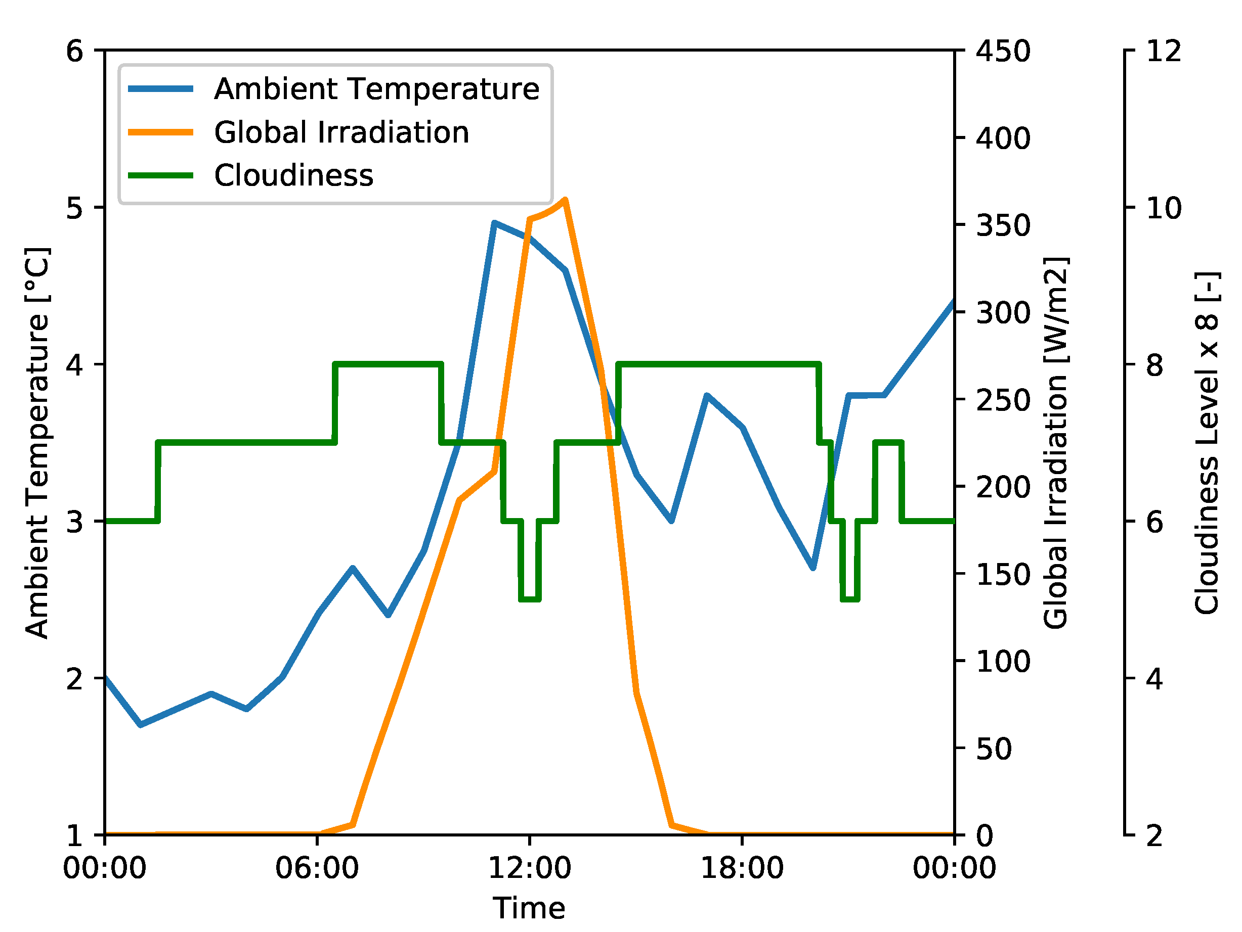
A winter cloudy type day is selected based on the VDI Standard 4655. The ambient weather temperature, the global solar irradiation, and the cloudiness are shown in Figure 4. According to the standard, the average temperature should be below 5 °C and the cloudiness should be higher than 5/8. On the selected day, the average temperature and cloudiness were 3.15 °C and 7/8, respectively. The number of cloudy winter days in the reference year was 85 days. The presented profile represents a typical average day of the given year in Munich, Germany. A winter type day is chosen to show clearly the influence of HiL on the quality of the results. A summer type day could have been selected, yet the space heating circuit would not be activated in this case. Hence, the HiL influence would not be noticed.

The heating circuit supply temperature is defined according to Equation (3), where ${\theta }_a$ is the ambient temperature. As shown, the supply temperature varies depending on the outside ambient temperature. The slope of the supply temperature is defined according to the recommended operation constraints and the nature of the building itself. Moreover, the required set temperature and user comfort level play an important role in deciding the slope of the heating curve. A change in the set temperature or the comfort level can be accompanied by a parallel shift of the heating circuit supply curve. As an example, if an increase in comfort is required, a parallel, upwards shift can be made. Alternatively, if the user needs to decrease the costs, the heating curve can be shifted downwards.

$${\theta }_{Supply,set}=\left\{\begin{array}{ll}50,& \mathrm{if}{\theta }_a<-20\\ -0.625\times {\theta }_a+37.5,& \mathrm{if}-20\le {\theta }_a\le 20,\\ 25,& \mathrm{if}{\theta }_a>20\end{array}\right.$$

(3)

4. Results and Analysis

In this paper, two cases are evaluated. The first case compares the testbed operation with and without HiL to present the added value and necessity of the HiL system. The comparison is based on energetic and dynamics analysis of the two experimental methods. The energetic analysis compares the energy consumption of the heat source and heat sink on the given type day. The dynamic analysis investigates and compares power and temperatures over time of the two experiments.

In the second case, the HiL system is used to validate a single family house model with a heat pump participating in an energy market. The preliminary market model was presented in [31]. The system dynamics evaluation of the model is crucial as it influences the time, volume and price of the heat pump energy bid in the market. Hence, a comparison is conducted between the HiL system and the model to evaluate and demonstrate the model accuracy.

4.1. Case 1: Testbed Operation with and without HiL

The goal of this case study is to evaluate the testbed operations with and without HiL to quantify the added value and present the necessity of the HiL systems. A reference load profile is generated from the building model using the type day presented in Section 3.4. The building model is connected to an over-sized heating source or a district heating to simulate the exact heat demand profile of the building without any compromises on the comfort side of the user.

Figure 5 presents the energy consumption and generation of the type day experiment, where $E_{el}$ is the electric energy consumption of the heat pump, $E_{th}$ is the thermal energy generation of the heat pump, $E_{brine}$ is the energy consumed on the brine side, and $E_{sh}$ is the energy consumed by the building. It can be seen that the deviation is between 0.2% to 5.5%, which is relatively small. However, it can be noticed that using the same metrics, the operation without HiL always has a lower consumption than the one with HiL. The reference space heating profile consumption is 132.8 kWh, compared to 135.3 kWh for the operation with HiL and 128.4 kWh for the operation without HiL. Although the experiment with HiL system is closer to the reference, it does not indicate a significant failure in the experiment without HiL. Hence, operating heating system testbeds without a HiL communication system has been widely accepted over the past years.

Insight on the dynamics and the difference between the testbed operations with and without HiL can be presented in Figure 6. Although the energy consumption is almost equal, a significant difference can be seen in the space heating dynamics between the operation with HiL, without HiL and the reference profile. Between 00:00 and 06:00 in Figure 6a, no differences can be noticed. The testbed operations are identical to the reference profile. With the increasing demand after 06:00 and the lack of sufficient energy in the heat storage, the power dropped. The testbed operation without HiL reaction was to reduce the return temperature trying to maintain the same power, as in Figure 6b. The return temperature, in this case, decreased to 17 °C, which is a major violation as the return temperature became lower than the room temperature. The testbed would have reduced the return temperature even to a lower level than 17 °C, but the cooling circuit capacity constrained it. On the other hand, the HiL system maintained a plausible return temperature due to the integration of a building model in the loop. Moreover, the HiL increased the thermal power after 08:00 to make up for the thermal power drop started at 06:00 and maintained a proper temperature, while the testbed operation without HiL continued to simulate the reference profile.

Another drop in power can be noticed between 12:00 and 18:00 for the HiL system. The testbed operating without HiL maintained the reference load profile power, even though there was not a sufficient amount of energy in the storage. This can be confirmed by the decrease in supply temperature noticed in Figure 6b. This drop is due to incapability of the heat pump to meet the demand. The HiL maintained a plausible return temperature, but return temperature without HiL decreased significantly. Although the power of the testbed operation without HiL seems acceptable, the return temperature dynamics are not realistic and can not be relied on for model validation or further research.

The behavior of the space heating circuit without HiL led to another operation plan for the heat pump, although the same control strategy is used. As in Figure 7, the heat pump started at the same time and behaved similarly within the first operation cycle. With the second cycle starting at 06:00, a difference can be seen that is increasing over time as seen at 15:00 and again at 20:00. This difference can lead to a significant error in the evaluation of energy management systems and cost optimization models based on variable electricity tariffs, or in energy market model as in Section 4.2. The exact operation plan represents a necessity in evaluating and validating the flexibility potential of heat pumps.

4.2. Case 2: Model Validation Based on HiL

Based on the model presented in [31], 10 single family residential houses are simulated located in Munich, Germany. These houses are participating in a local energy market, where each device sell or buy energy depending on its operation mode. Each house is equipped with a photovoltaic system, an electric vehicle and a heat pump. The installed PV capacity at each house is 6 kWp. The technical details and the data of the integrated PV system can be found in [34]. A 3.6 kW charging station is used for the electric vehicle, while the integrated heat pump is represented by the testbed in Section 3.2. More details about the heat pump testbed can be found in [15]. A single family house is selected from these 10 houses to be validated based on the HiL system and the heat pump testbed.

The goal of the model validation is to compare the operation of the heat pump in the model to the testbed with HiL while making sure that the building load is covered and the room temperature is properly maintained. On the heat sink side, Figure 8a shows that the space heating power of the testbed with HiL and the simulation are behaving similarly. Even when a drop in the thermal power occurred at 17:00, it did not influence the room temperature as shown in Figure 8c. The room temperatures of the completely simulated model and HiL are showing similar dynamics. A difference can be noticed between 09:00 to 22:00, yet this difference is below 0.02 °C. In Figure 8b, the supply and return temperature of the HiL testbed and simulation model can be compared. The supply temperature is varying based on the supply curve earlier defined in Equation (3). It can be seen that the supply temperature shows plausible results except at 17:00, where a drop in the temperature can be noticed because of the low storage content. An operation without HiL would have led to a proportional decrease in the return temperature, yet the HiL system maintained realistic dynamics. Comparing the model to the HiL, it can be noticed that the return temperatures are not violated, and both the HiL and simulation dynamics are comparable except at the starting point, where minor fluctuation occurred by the simulation solver. In the HiL measurements, spikes can be noticed to due few data packet losses ín the communication between the testbed and model. However, it does not influence the overall results.

The behavior of the heat pump in the HiL and simulation is almost identical as in Figure 9. The magnitude of the thermal and electrical power is equivalent, which means that the heat pump has been providing power to the heat storage almost at the same supply temperature. In this type day, the energy difference between the HiL system and the simulation is 2% and 5% for the heat generation and electricity consumption, respectively. However, the HiL based validation in this paper does not only concern the energetic consumption but also the temporal distortion of the power. The time and volume of the heat pump bid in an energy market have to be evaluated to validate the accuracy of the model.

In [15], the thermal and electrical power of the heat pump model were validated independently based on mean absolute percentage error (MAPE) and root mean square error (RMSD). However, since the temporal distortion of the model compared to the HiL is crucial to evaluate the model capability in participating in energy markets at the estimated times, the temporal distortion index (TDI) of [35] is used. This metric is based on the dynamic time warping (DTW) developed in the 1970s, which is used to evaluate the temporal distortion between two different time series. In this paper, the two time series are the HiL measurements and simulation model time series of the heat pump electrical power. The DTW finds the optimal warping path (i.e., a common set of instants) by minimizing the distance between the two given time series. The TDI can be calculated then according to Equation (4), where i and j are the HiL measurements time series index and simulation model time series index, respectively.

$$TDI={\displaystyle \frac{1}{N^2}}\sum _{l=1}^{k-1}\left|(i_{l+1}-i_l)(i_{l+1}+i_l-j_{l+1}-j_l)\right|$$

(4)

The output of the TDI is between 0 and 1. The lower the value of the TDI metric, the lower is the temporal distortion. The metric result in this type day is 3%, which means that temporal distortions between the HiL measurements and the simulation model are low.

5. Conclusions

In this paper, hardware in the loop (HiL) real-time system is presented. The HiL communication structure, models and testbeds are explained to show the experimental setup of HiL for heating systems. Two case studies are demonstrated to evaluate the potential and applications of the HiL. The first case study evaluates the energy consumption and dynamics of the testbed operation with and without HiL. The results of the case study are summarized as follows:

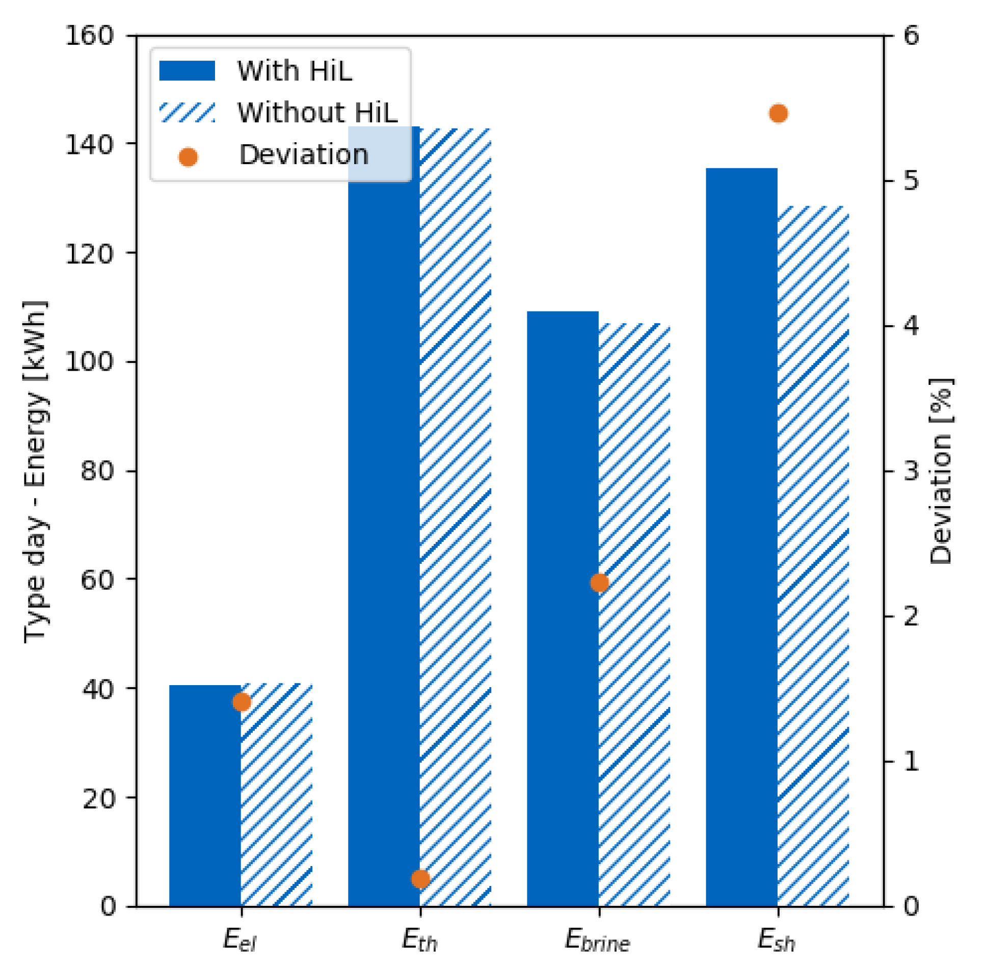
• Testbed operation with or without HiL does not influence the heat energy consumption of the heat sink (space heating), or the heat energy generation from the heat pump. The variations in results are between 0.2% and 5.5%. Hence, energetically no significant difference can be noticed.
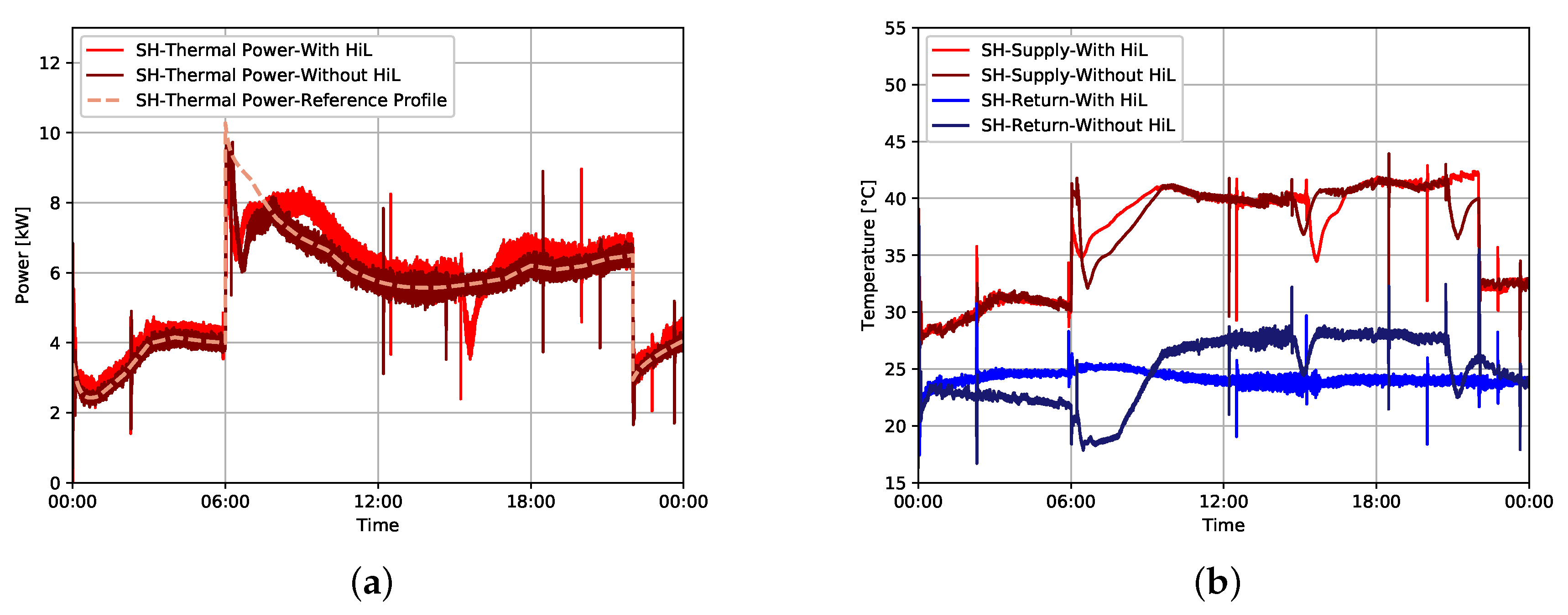
• The dynamics of the testbed operation without HiL showed that a drop in the space heating supply temperature is always accompanied by an equivalent drop in the return temperature of the space heating. Thus, testbed operation without HiL can not emulate real-life return temperature dynamics and can lead to system violations.
• The HiL system is able to maintain realistic dynamics due to the availability of a building model in the loop.
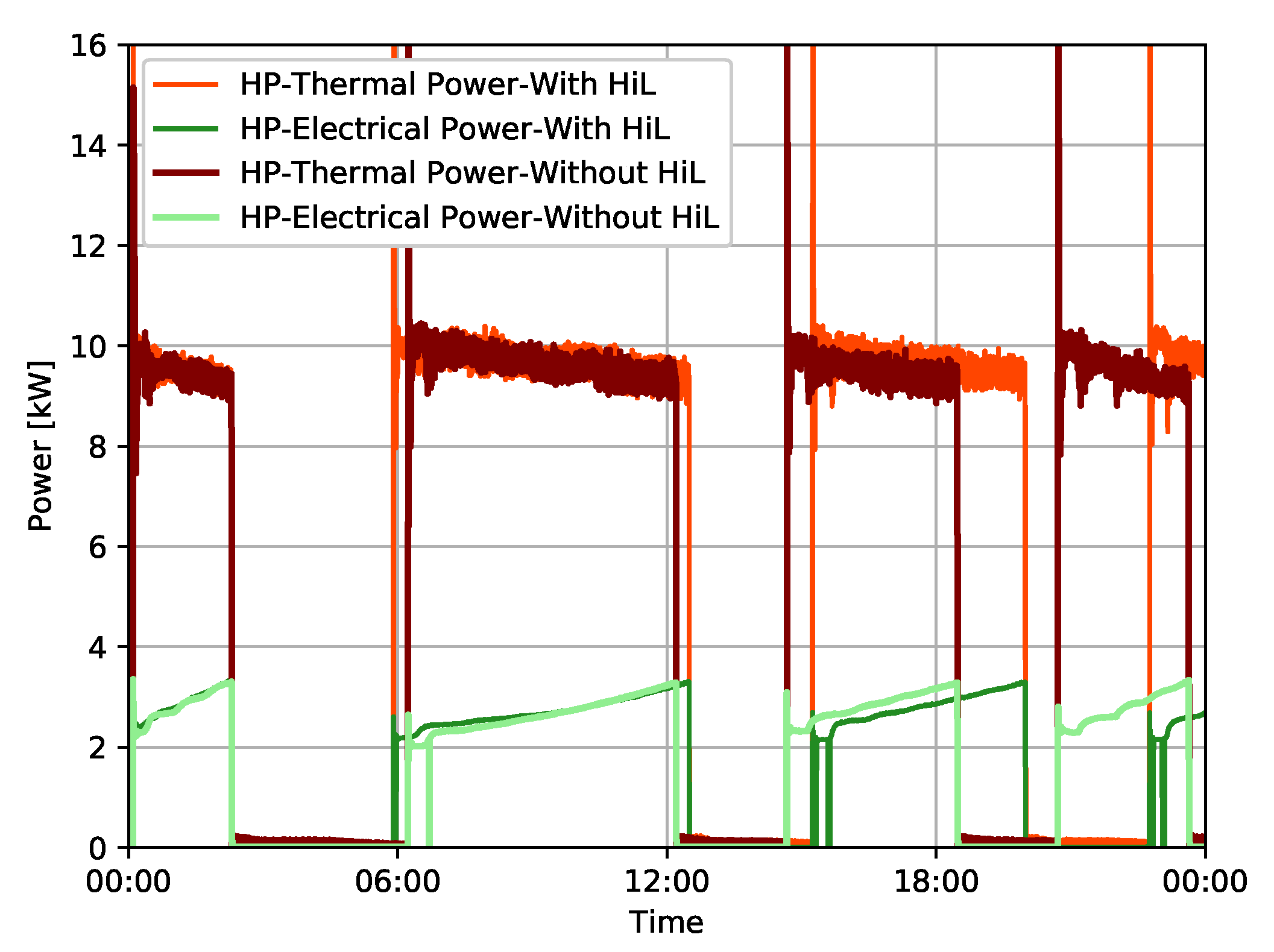
• The violations of the testbed operation without HiL led to a shift in the operation plan of the heat pump. Hence, the testbed operation without HiL is not reliable for heating system models validation.

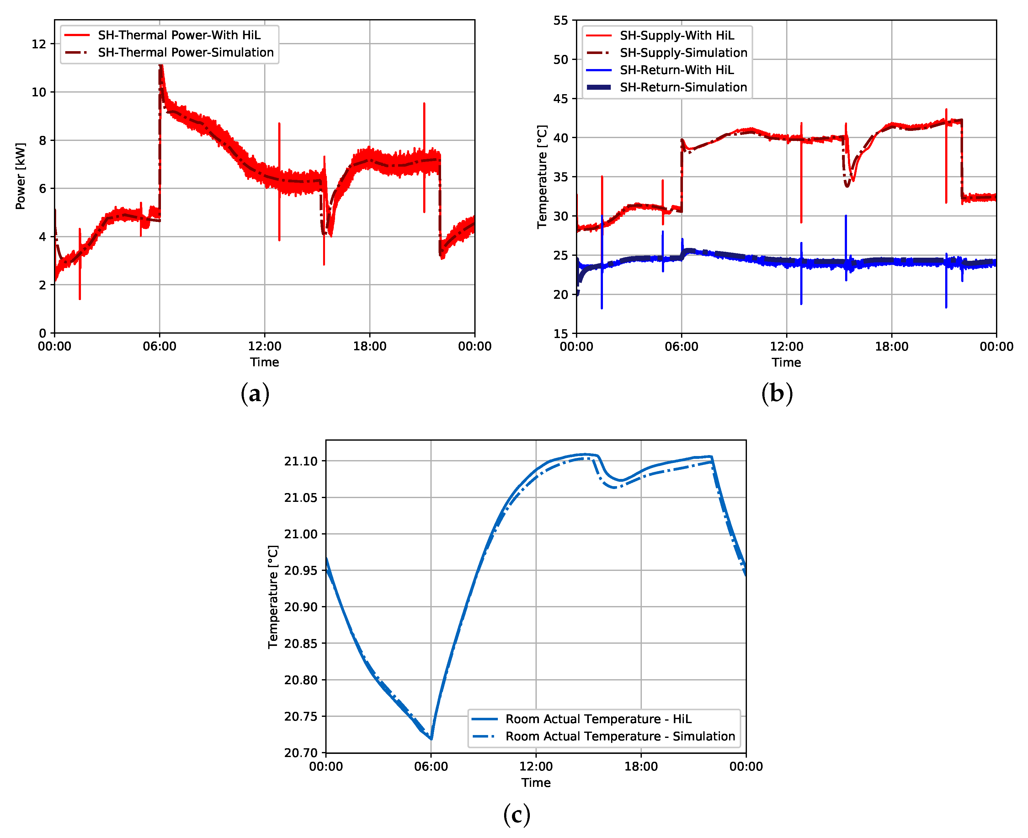
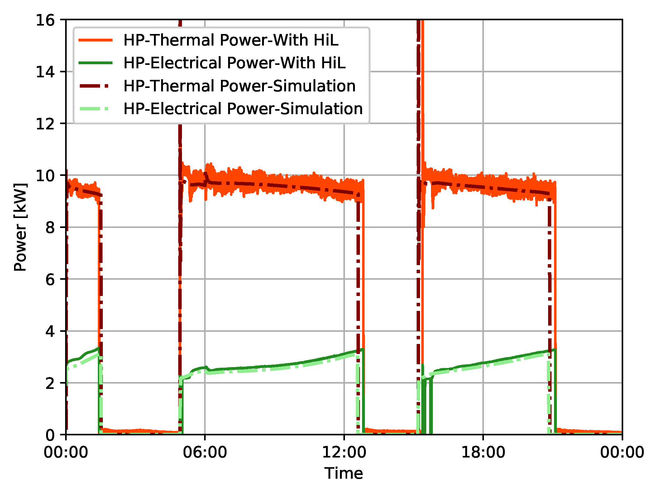
In the second case study, the HiL system is used to validate a single family house building participating in a local energy market. HiL is chosen as it is necessary to validate not only the energy consumption but also the system dynamics and the temporal distortion of the model. The simulation model showed its capability to present the heat pump system dynamics including any drops in the supply temperature or the heat storage of the tank. The HiL also showed the advantage of demonstrating the room temperature of the building model for the given type day, which facilitates evaluating the comfort of the residents and comparing it to the simulation model. Furthermore, TDI is used to quantify the temporal distortion of the heat pump to make sure that the electric energy consumption is communicated at the right time of the day. The TDI value is 3%. Hence, a minimal temporal distortion can be noticed between the HiL and the simulation model.

As an outlook, HiL for heating systems can be used for several further studies. It enables not only an accurate validation of a simulation model but also experimentation using a building model inertia to offer flexibility to the grid. The HiL can also be further developed to include multiple heating systems that can communicate and interact in the same local heating network or microgrid.