Robust Optimization of Power Consumption for Public Buildings Considering Forecasting Uncertainty of Environmental Factors

Abstract

In recent years, with the advancement of urban construction in China, the optimization of power consumption in public buildings has been focused on. The optimization of power consumption in public buildings is based on the prediction of natural illuminance, outdoor air temperature and flow of people in public building. Therefore, it is worthwhile to study how to formulate a power consumption strategy with consideration of forecasting uncertainty of environmental factors. The robust-index method is proposed to deal with the problem of forecasting uncertainty. Firstly, this paper establishes power consumption models for lighting systems, air-conditioning systems, and elevator systems in public buildings. Secondly, the robust indexes for each system and the synthetic robust index are established. Thirdly, the objective function is formulated to reduce the total electricity cost with the robust indexes applied as additional constraints to the optimization problem, therefore the obtained power consumption schedules are able to reach the expected robust level. Finally, simulation results show attributes of the proposed method.

1. Introduction

With the increasing pressure on global resources and the environment, more and more people are concerned about the problem of energy efficiency. In order to solve these problems, the global electric-power industry has gradually entered the era of the smart grid, and the main feature of the smart grid is that the power resources can be configured in a comprehensive way. Therefore, in the field of energy management, the concept of intelligent power consumption is put forward. It means to take effective measures to guide and optimize the power consumption for power users, so as to promote energy efficiency and achieve the minimum electricity payments [1,2]. According to statistics, buildings make up 33% of the total Chinese energy consumption [3]. Therefore, it is of great practical value to research the problem of load scheduling in public buildings to reduce the total electricity cost of public buildings and bring down the power consumption.

In recent years, the power consumption strategy of public buildings has been extensively studied. In [4], a GA (genetic algorithm) optimization framework based on high-throughput distributed computation environment is proposed to reduce the cost and computation time of complex building energy optimization. Reference [5] studied the scheduling problem of large-scale smart appliances and batteries to minimize electricity cost, customers’ dissatisfaction and battery loss under the constraints. In [6], the models of conventional residential controllable loads were built and aggregated to generate the load profiles for DR (demand response) research. In [7], the optimization schedule of electric water heating was studied in response to the time-of-use price with the goal of minimizing the electrical cost. In [8], an intelligent HEM (home energy management) algorithm for managing the power consumption of households was studied, which managed household loads in accordance with their preset priority and guaranteed the whole power consumption below a certain level. The above research built models for household appliances and studied the load schedules in order to minimize the total electricity payments, however, the problem of forecasting uncertainty of environmental factors was not considered.

Due to a variety of factors, there is a deviation between the forecasting data and the actual data, and the uncertainty of the forecasting data may cause some losses to the customers. Reference [9,10,11] modeled the uncertainties of renewable resources such as wind and solar energy. Reference [12,13,14] studied the load scheduling with the consideration of electricity price uncertainty. Reference [15,16] researched the load output uncertainty for optimization. Reference [17,18] dealt with the uncertainty problem by employing the robust optimization method. In [19], a robust optimization method was proposed to tackle the uncertainty problem of customer behavior, which was more effective than the traditional robust methods. However, to the best of our knowledge, there are no studies of a power consumption strategy for public buildings considering forecasting uncertainty of environmental factors (nature illuminance, outdoor air temperature, and flow of people in the building) up to the present time.

Based on such a background, this paper studies robust optimization for a power consumption strategy for public buildings, also considering the forecasting uncertainty of environmental factors. The power consumption models of the lighting systems, air-conditioning systems, and elevator systems in public buildings are built firstly. Then, considering the uncertainty of environmental factors’ (nature illuminance, outdoor air temperature, and people flow of public buildings) prediction, a robust index of each system is built. Thirdly, the robust optimization model for electricity consumption considering the forecasting uncertainties of environmental factors in public buildings is established to minimize the total electricity cost and to satisfy user comfort. Finally, simulation results show attributes of the proposed method.

The main contributions of this paper are summarized as follows:

(1)

The energy consumption of lighting systems, air-conditioning systems, and elevator systems in public buildings is analyzed. The relationship between energy consumption and the external variables of the lighting system, air-conditioning system, and elevator system are modeled, respectively.

(2)

Considering the forecasting uncertainty of environmental factors (outdoor illuminance, temperature, and the flow of people in buildings), the robust indexes of the lighting system, air-conditioning system, and elevator system are established, respectively, and the synthetic robust index in public buildings is established.

(3)

A robust optimization model for power consumption in public buildings considering the forecasting uncertainty of environmental factors is established by robust indexes, with the objective of optimizing the total electricity cost and satisfying the users’ comfort.

The rest of this paper is organized as follows. Section 2 describes the modeling of the lighting system, air-conditioning system, and elevator system. Section 3 introduces the robust-index for modeling the forecasting uncertainty of environmental factors. Illustrative case studies are presented in Section 4 and the paper is concluded in Section 5.

2. Modeling the Electric Energy Consumption of Public Buildings

The electric energy consumption models for the lighting system, air-conditioning system, and elevator system in public buildings were built in this section.

2.1. Lighting System

The indoor average illuminance is calculated by the following Equation (1):

$$E_{av}=\frac{\varphi NUK}{A}$$

(1)

where E_av is average illuminance, $\varphi$ is the luminous flux, N is the number of lamps, U is the utilization coefficient, K is the maintenance coefficient of lamps, and A is the illuminated area.

Generally, we need to maintain indoor illuminance above a certain level to ensure working environment comfort, that is, the superposition of natural light and artificial light should meet the indoor demand. As a result, the lighting load can be determined by the following Equation (2):

$$P_{l,t}=\{\begin{array}{cc}\frac{\left(E_{set}-E_e\right)A}{\varphi UK}{P}_l,& t\in t_{work}\\ 0,& t\notin t_{work}\end{array}$$

(2)

where P_l,t is the power consumption at the end of the tth time slot, E_set is the target illuminance, E_e is the natural illuminance, P_l is the power of one lamp.

2.2. Air-Conditioning System

Without loss of any generality, this paper considers the power consumption of air-conditioning in summer, and the main sources of heat are through the exterior wall and the roof, the glass window, the human body heat dissipation, lighting, and heat dissipation. The cooling load of a public building is the cooling required to maintain the indoor temperature by the air-conditioning system, and the cooling load includes the following parts:

(a)

Heat from the roof and exterior wall

$$Q_1=KA\left(T_{out}-T_{in}\right)$$

(3)

where K is the heat transfer coefficient of the fence structure, A is the heat transfer area of the fence structure, T_out and T_in are the inside and outside temperature, respectively.

(b)

Solar radiation heat from glass windows

$$Q_2=C_{a}A{C}_s{C}_i{D}_{j\max }{C}_{LQ}$$

(4)

where C_a is the effective area coefficient, A is window area, C_s is the sun shading coefficient, C_i is the shading coefficient, D_jmax is the maximum solar radiation heat, and C_LQ is the cooling load coefficient of window glass.

(c)

Heat dissipation of bodies

$$Q_3=q_{s}n\psi C_{LQ}$$

(5)

where q_s is the sensible heat gain for male adults, n is the total number of people in the building, ψ is the cluster coefficient, and C_LQ is the cooling load coefficient for sensible heat gain from human bodies.

(d)

Heat dissipation of lamps

$$Q_4=1000P_l{C}_{LQ}$$

(6)

where P_l is the power required for lighting, C_LQ is the cooling load coefficient of lamps.

(e)

Load of fresh air

In the air-conditioning system, the inclusion of outdoor fresh air is important to guarantee indoor air quality. The load of fresh air is calculated with the following Equation (7):

$$Q_5=M(h_{out}-h_{in})$$

(7)

where M is the quantity of fresh air, h_out is the outdoor air enthalpy, h_in is the indoor air enthalpy,

The enthalpy of air is the enthalpy of dry air in moist air and the enthalpy of water vapor, which includes sensible heat and latent heat. It can be calculated as the following Equation (8):

$$h=1.01T+d(2500+1.84T)$$

(8)

where d indicates the moisture content, usually d = 0.014 kg/(kg dry air).

M is calculated with the following Equation (9):

$$M=R_p\times n+R_b\times s$$

(9)

where R_p is the minimum fresh air per person, R_b is the minimum fresh air for each square meter, n is number of people, and s is the building area.

To conclude, the cooling load can be determined by the following Equation (10):

$$\begin{array}{l}Q=KA\left(T_{out}-T_{in}\right)+C_{a}A{C}_s{C}_i{D}_{j\max }{C}_{LQ}+q_{s}n\psi C_{LQ}+\\ 1000P{C}_{LQ}+M(R_p\times n+R_b\times S)(h_{out}-h_{in})\end{array}$$

(10)

And the power consumption of the water chiller is formulated with the following Equation (11):

$$x_{a,t}=\frac{Q_{}}{COP}$$

(11)

where x_a,t is the power consumption of the air-conditioning system at the tth time slot, Q is the cooling load, and COP is the coefficient of performance.

2.3. Elevator System

For public buildings, there lies regularity to some extent in the operation time and usage habits of elevators, and the operation modes of elevator system can be divided into three kinds: (a) up-peak mode: upward passenger flow is far greater than downward passenger flow. This mode usually occurs in the morning working hours; (b) down-peak mode: the main passenger flow is in the downward direction. The main flow is from the building floor down to leave the building, and this mode generally occurs in the evening off-duty hours; (c) off-peak mode: upstream and downstream passenger flow is stable, and there is no dominant passenger flow. This mode occupies the majority of working hours.

There are usually several elevators running at the same time in their operating period. The power consumption of the elevator system is directly related to the scale of the human flow and the number of operating elevators. According to the data measured in [20], the power consumption can be calculated with the following Equation (12):

$$E_{LF}\left(\tau \right)=a+b_1{F}_{P,\tau }+b_2{N}_{car,\tau }+b_3{F}_{P,\tau }{N}_{car,\tau }+b_4{\left(F_{P,\tau }\right)}^2+b_5{\left(N_{car,\tau }\right)}^2$$

(12)

where E_lf is the power consumption and F_p,τ and N_car,τ are the flow of people and number of elevators, respectively.

Then, the energy consumption models for the elevator system under different operation modes can be described as follows.

(a) Up-peak mode

The energy consumption under up-peak mode is calculated with the following Equation (13):

$$\begin{array}{cc}\hfill E_{LF}\left(\tau \right)& =365.32-1.115F_{P,\tau }-0.199N_{car,\tau }+0.143F_{P,\tau }{N}_{car,\tau }\hfill \\ & +0.087F_{P,\tau }{}^2-0.228N_{car,\tau }{}^2\hfill \end{array}$$

(13)

The flow of people is constrained from Equations (14):

$$\{\begin{array}{c}{P}_{u,\tau }\ge 0.85F_{P,\tau }\\ 0.8P_{u,\tau }\le x_{D,u,\tau }^{in}\le P_{u,\tau }\\ 0.55x_{D,u,\tau }^{in}\le x_T^{out}\le P_{u,\tau }\\ 0\le P_{d,\tau }\le 0.15F_{P,\tau }\end{array}$$

(14)

where P_u,τ is the up flow, P_d,τ is the down flow, $x_{D,u,\tau }^{in}$ is the up flow from the first floor, and $x_T^{out}$ is the down flow from the highest floor.

The average waiting time is calculated with the following Equation (15):

$$\begin{array}{ll}{T}_{AW}\left(\tau \right)& =600.403-359.239\ln \left(F_{P,\tau }\right)+86.113\ln \left(N_{car,\tau }\right)\\ & -57.995\ln \left(F_{P,\tau }{N}_{car,\tau }\right)+62.096\ln {\left(F_{P,\tau }\right)}^2+36.007\ln {\left(N_{car,\tau }\right)}^2\end{array}$$

(15)

(b) Down-peak mode

The energy consumption under down-peak mode is calculated with the following Equation (16):

$$\begin{array}{ll}{E}_{LF}\left(\tau \right)& =-523.806+30.355F_{P,\tau }-14.123N_{car,\tau }+0.241F_{P,\tau }{N}_{car,\tau }\\ & -0.188F_{P,\tau }{}^2+0.774N_{car,\tau }{}^2\end{array}$$

(16)

The flow of people is constrained from Equations (17):

$$\{\begin{array}{c}{P}_{d,\tau }\ge 0.85F_{P,\tau }\\ 0.8P_{d,\tau }\le x_{T,d,\tau }^{in}\le P_{d,\tau }\\ 0.55x_{T,d,\tau }^{in}\le x_D^{out}\le P_{d,\tau }\\ 0\le P_{u,\tau }\le 0.15F_{P,\tau }\end{array}$$

(17)

The average waiting time is calculated with the following Equation (18):

$$\begin{array}{ll}{T}_{AW}\left(\tau \right)& =729.197-429.455\ln \left(F_{P,\tau }\right)+99.519\ln \left(N_{car,\tau }\right)\\ & -54.286\ln \left(F_{P,\tau }{N}_{car,\tau }\right)+69.213\ln {\left(F_{P,\tau }\right)}^2+29.390\ln {\left(N_{car,\tau }\right)}^2\end{array}$$

(18)

(c) Off-peak mode

The energy consumption under off-peak mode is calculated with the following Equation (19):

$$\begin{array}{ll}{E}_{LF}\left(\tau \right)& =276.885-5.409F_{P,\tau }-4.1N_{car,\tau }+0.067F_{P,\tau }{N}_{car,\tau }\\ & +0.058F_{P,\tau }{}^2+0.321N_{car,\tau }{}^2\end{array}$$

(19)

The flow of people is constrained from Equation (20):

$$\{\begin{array}{c}{P}_{d,\tau }<0.85F_{P,\tau }\\ P_{u,\tau }<0.85F_{P,\tau }\\ 0.8\le P_{u,\tau }/P_{d,\tau }\le 1.25\end{array}$$

(20)

The average waiting time is calculated with the following Equation (21):

$$\begin{array}{ll}{T}_{AW}\left(\tau \right)& =622.589-352.932\ln \left(F_{P,\tau }\right)+56.316\ln \left(N_{car,\tau }\right)\\ & -43.369\ln \left(F_{P,\tau }{N}_{car,\tau }\right)+56.403\ln {\left(F_{P,\tau }\right)}^2+30.878\ln {\left(N_{car,\tau }\right)}^2\end{array}$$

(21)

As the degree of anxiety of passengers increases with the increase of waiting time. Therefore, the average waiting time of passengers can be used to evaluate passengers’ satisfaction with the elevator system.

2.4. Objective of the Power Consumption Optimization Problem of Public Building

Cost minimization is usually chosen as the objective function of power consumption optimization of public buildings. In this paper, the optimization goal is to minimize the electricity cost of the public buildings, so the optimization problem for power consumption optimization is obtained with the Equation (22):

$$\min {\displaystyle \sum _{t=1}^h{P}_t}\cdot x_t$$

(22)

where P_t is the electricity price at the tth time slot, x_t is the whole electric power consumption of lighting system, air-conditioning system and elevator system.

2.5. Constraints of the Power Consumption Optimization Problem of Public Building

The constraints of the power consumption optimization problem of public buildings are as follows:

The constraints of the lighting system: (1) and (2).

The constraints of the air-conditioning system: (3)–(11).

The constraints of the elevator system: (13)–(21).

The constraints of the customers’ comfort for the lighting system are imposed by the Equation (23):

$$E_{\min }\le E_{set}\le E_{\max }$$

(23)

The constraints of the customers’ comfort for the air-conditioning system are imposed by the Equation (24):

$$T_{\min }\le T_{set}\le T_{\max }$$

(24)

The constraints of the customers’ comfort for the elevator system are imposed by the Equation (25):

$$X_{\min }\le X_{set}\le X_{\max }$$

(25)

3. Robust-Index for Electric Energy Consumption Systems

The forecasting accuracy of environmental factors will have a great impact on the optimization results, so the robust-index is employed to analyze the uncertainty of the prediction of environmental factors. The higher the robust index is, the stronger the robustness of the optimization result would be, that is, fewer negative impacts of uncertainties would occur. The robust indexes are applied as additional constraints to the power consumption optimization problem of public buildings.

3.1. Lighting System

The robust index for the lighting system is calculated by the following Equation (26):

$$E_{l,pre}-E_{l,sup}=R{I}_l\ge R{I}_{l,set}$$

(26)

where E_l,pre is the outdoor illuminance under deterministic prediction, E_l,sup is the supposed illuminance in power consumption optimization, RI_l is the robust index of the lighting system, and RI_l,set is the minimum robust index value needed.

Suppose the outdoor illuminance under interval prediction is [E_l,min, E_l,max], which is the range of E_l,sup. The maximum and minimum value of robust index RI_l are respectively calculated by the following Equations (27) and (28):

$$R{I}_{l,\max }=E_{l,\max }-E_{l,\min }$$

(27)

$$R{I}_{l,\min }=0$$

(28)

3.2. Air-Conditioning System

The robust index for the air-conditioning system is calculated by the following Equation (29):

$$T_{a,\sup }-T_{a,pre}=R{I}_a\ge R{I}_{a,set}$$

(29)

where T_a,pre is the outdoor temperature under deterministic prediction, T_a.sup is the supposed temperature in power consumption optimization, RI_a is the robust index of the air-conditioning system, and RI_a,set is the minimum robust index value needed.

Suppose the outdoor temperature under interval prediction is [T_a,min, T_a,max], which is the range of T_a,sup. The maximum and minimum value of robust index RI_a are respectively calculated by the following Equations (30) and (31):

$$R{I}_{a,\max }=T_{a,\max }-T_{a,\min }$$

(30)

$$R{I}_{a,\min }=0$$

(31)

3.3. Elevator System

The robust index for the elevator system is calculated by the following Equation (32):

$$F_{p,\sup }-F_{p,pre}=R{I}_p\ge R{I}_{p,set}$$

(32)

where F_p,pre is the flow of people under deterministic prediction, F_p,sup is the supposed flow in power consumption optimization, RI_p is the robust index of the elevator system, RI_p,set is the minimum robust index value needed.

Suppose the flow under interval prediction is [F_p,min, F_p,max], which is the range of F_p,sup. The maximum and minimum value of robust index RI_p are respectively calculated by the following Equations (33) and (34):

$$R{I}_{p,\max }=F_{p,\max }-F_{p,\min }$$

(33)

$$R{I}_{p,\min }=0$$

(34)

3.4. Normalization of Robust Index

The units of the robust index for each sub electric energy utilization system are different, and thus it is difficult to compare the robustness of each system. Therefore, the robust index of each sub electric energy utilization system should be normalized with the range of [0, 1]. Each robust index is normalized by the following Equation (35):

$$R{I}_N=\frac{R{I}_{raw}-R{I}_{\min }}{R{I}_{\max }-R{I}_{\min }}$$

(35)

where RI_N is the normalized robust index, RI_raw is a raw robust index before normalization, and RI_max and RI_min are the maximum and minimum values of corresponding raw robust indexes.

3.5. Synthetic Robust Index

The robust indexes of different sub electric energy utilization systems are established above. In order to evaluate the overall robust level of the public buildings, the synthetic robust index is proposed. The synthetic robust index can be expressed with a weighted sum the with Equations (36) and (37):

$${\displaystyle \sum _{\delta }{v}_{\delta }}\cdot R{I}_{\delta }=R{I}_{mix}\ge R{I}_{req}$$

(36)

$$v_{\delta }\in \left[0,1\right],{\displaystyle \sum _{\delta }{v}_{\delta }}=1$$

(37)

where v_δ is the weighted coefficient of sub electric energy utilization system δ, and it reflects the importance of the sub electric energy utilization system, RI_mix is the synthetic robust index. In addition, the synthetic robust index is less than RI_req, which reflects the overall robustness level of public buildings.

4. Numerical Examples

The proposed method is tested using numerical experiments. Firstly, the robust indexes for different power consumption systems are validated. Secondly, a comprehensive simulation is conducted to demonstrate the application of synthetic robust indexes.

4.1. Initial Data

There are many kinds of public buildings, such as office buildings, hotels, supermarkets, etc. The actual data in this paper are collected from one office building in Suzhou City, Jiangsu Province, P. R. China. The working hours of a public building are 9:00–21:00 and Δt = 1 h. The lighting system is made up of LED lamps, and the lighting area is 17,768 m². The lighting power per unit area is 3 W with the luminous flux 100 mL/W. The lighting utilization coefficient is 0.5 and the lighting maintenance coefficient is 0.8. The total cooling area for the air-conditioning system is 17,768 m² and the total exterior wall area of the public building is 7000 m². The average window–wall ratio is 0.38. In addition, there are 8 elevators in this building.

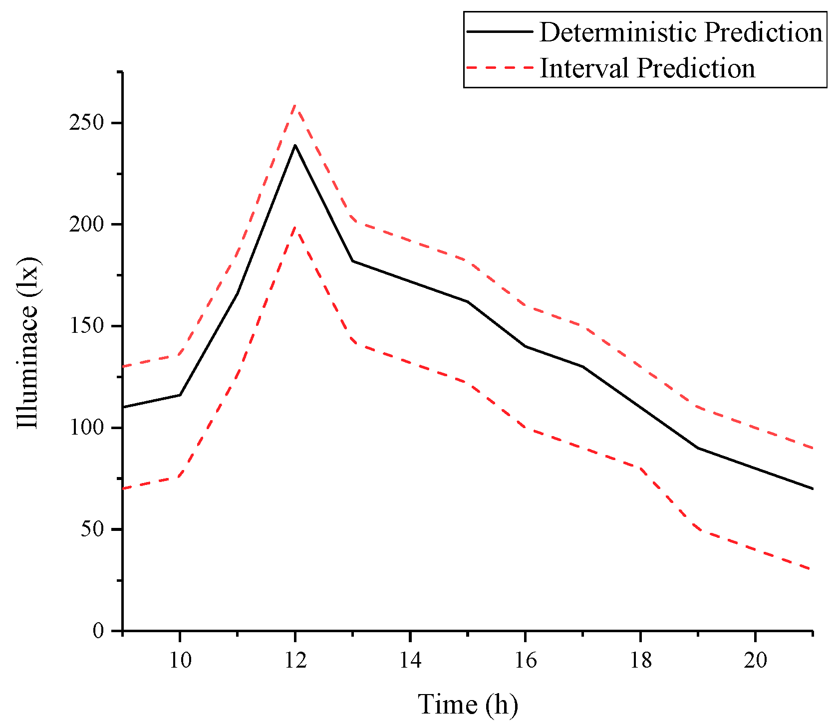
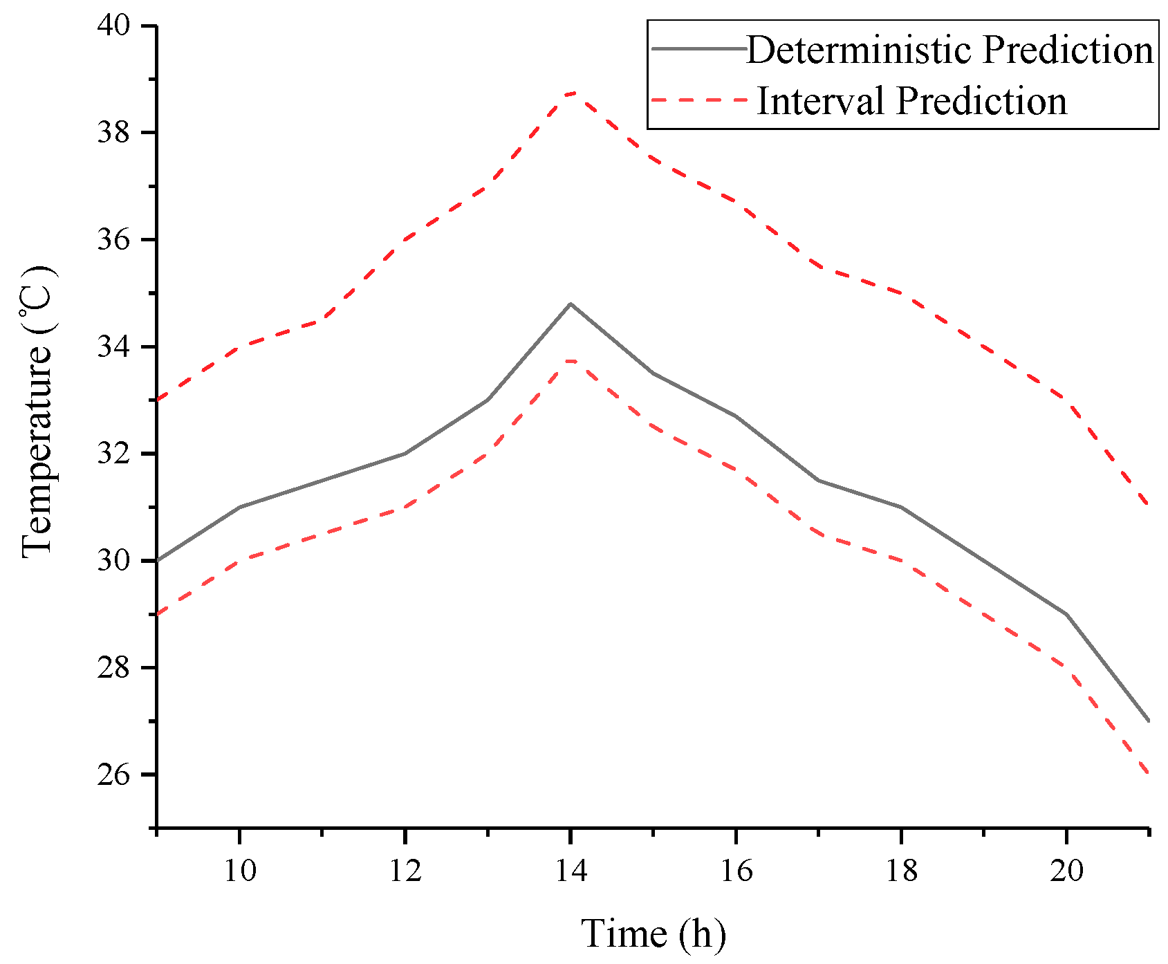
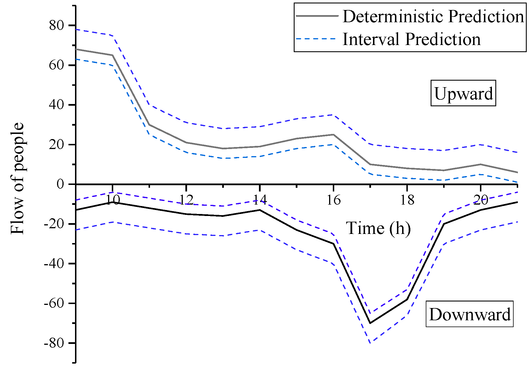
Reference [21,22,23] use probabilistic model to study the problem of uncertainty. However, the robust index model employs the interval values of the variables to calculate the maximum and minimum index values, so this paper use intervals of random variables rather than probability distribution of random variables. The forecasting of natural illuminance, outdoor temperature, and human flow are shown in Figure 1, Figure 2 and Figure 3, respectively.

4.2. Simulations

First, the robust level considering forecasting uncertainties of each sub electric energy utilization system is evaluated. The robust indexes for different power consumption systems are simulated.

The electricity cost of the lighting system under different robust indexes is shown in

Table 1. Electricity cost under different robust indexes of the lighting system.

RIN-set	Cost/¥
0	942.95
0.05	959.83
0.1	976.7
0.15	993.58
0.2	1010.46
0.25	1027.33

. The load schedule of this system is solved by the optimization model that consists of objective function (22) (without consideration of other systems), comfortable constraint Equation (23), and robust index constraint (26). Equations (1) and (2) are taken as the constraints to calculate the electricity consumption of the lighting system. As can be seen from Table 1, the electricity cost of the lighting system increases with the increase of the robust index. Since the feasible area of the electric energy utilization optimization become smaller with the increase of the level of robustness, the more illuminance the indoor environment requires, the higher the cost.

The electricity cost of the air-conditioning system under different robust indexes is shown in

Table 2. Electricity cost under different robust indexes of the air-conditioning system.

RIN-set	Cost/¥
0	2127.49
0.1	2132.75
0.2	2138
0.3	2134.81
0.4	2149.61
0.5	2155.41
0.6	2161.21
0.7	2167
0.8	2172.8
0.9	2178.6
1	2184.4

. The load schedule of this system is solved by the optimization model that consists of the objective Equation (22) (without consideration of other systems), comfortable constraint (24), and robust index constraint (29). Equations (3)–(11) are taken as the constraints to calculate the electricity consumption of the air-conditioning system. As the robust index increases, the cost gradually increases. This is because the air-conditioning system consumes more electric energy to keep the temperature lower; as a result, the forecasting uncertainty of environmental factors can be dealt with more robustly. It can be seen that the improvement of system robustness is accompanied with the reduction of economy. This paper considers customers’ comfort by setting the temperature ranges in advance. In fact, there are several studies on customers’ comfort [24,25] and new eco-sustainable technologies such as the use of smart windows and innovative plant systems [26,27].

For the elevator system, this paper only focuses on the up-peak and down-peak modes.

Table 3. Electricity cost under different robust indexes of the elevator system (up-peak mode).

RIN-set	Cost/¥
0	918.02
0.1	929.11
0.2	940.2
0.3	951.29
0.4	962.38
0.5	973.47
0.6	984.56
0.7	995.65
0.8	1006.74
0.9	1017.83
1	1028.92

and

Table 4. Electricity cost under different robust indexes of the elevator system (down-peak mode).

RIN-set	Cost/¥
0	756.61
0.1	791.65
0.2	826.69
0.3	861.72
0.4	896.76
0.5	931.79
0.6	966.83
0.7	1001.86
0.8	1036.9
0.9	1071.94
1	1106.97

show the electricity cost of the elevator system under different robust indexes in the up-peak hours and down-peak hours, respectively. The load schedule of this system is solved by the optimization model that consists of the objective function Equation (22) (without consideration of other systems), comfortable constraint Equation (25), and robust index constraint Equation (32). Equations (13)–(21) are taken as the constraints to calculate the electricity consumption of the elevator system. According to Table 3 and Table 4, the electricity cost of the elevator system increases with the increase of the robust index. This is because the larger the robust index is, the more frequently the elevators would be operated to meet the running requirements for more people, however, this incurs a greater electricity bill.

Then, to demonstrate the application of synthetic robust indexes in the load schedule, a comprehensive simulation is designed. Equation (22) is taken as the objective function, and the equations in Section 2 are taken as the constraints to calculate the electricity consumption of different loads. Equations (36) and (37) are taken as the additional index robust constraint, which are derived from (26)–(35).

Considering the synthetic robust level of public buildings, three different cases are designed for contrast. The weighted coefficients of each system are presented in

Table 5. Weighted coefficient of each system in different scenes.

Case	Weighted Coefficient
	Lighting	Air-Conditioning	Elevator
1	0.3	0.4	0.3
2	0.3	0.4	0.3
3	0.6	0.3	0.1

and the synthetic robust indexes are presented in the last column of

Table 6. Robust index values of different systems.

Case	Robust Index Values
	Lighting	Air-Conditioning	Elevator	Synthetic
1	0.05	0.43	0.05	0.2
2	0.05	1	0.28	0.5
3	0.325	1	0.05	0.5

.

Table 7. Total electricity cost.

Case	Cost/¥
1	4553.26
2	4626.83
3	4681.87

shows the electricity cost under different cases.

Firstly, Case 1 and Case 2 are compared. Case 1 and Case 2 set the same weighted coefficients, and the synthetic robust indexes are required to be 0.2 and 0.5, respectively. Then, we can obtain robust indexes of each power consumption system and analyze the impact of different synthetic robust index setting. From Table 6, it can be seen that the higher the synthetic robust index is, the higher the robust index of each systems will be, and the cost charge will also increase from Table 7. This is because, with the increase of the synthetic robust index, electric energy utilization systems can cope with the forecasting uncertainty of environmental factors better and sacrifice economy to improve robustness.

Secondly, Case 2 and Case 3 are compared. Case 2 and Case 3 set the same synthetic robust index (0.5) and set different weighted coefficients. Then, we can obtain robust indexes of each power consumption system and analyze the impact of different weighted coefficients. As shown in Table 6, the robust indexes of each system change with different load weighted coefficients, which indicates that the difference in sub electric energy utilization system weight affects the power consumption optimization.

In addition, the costs of Case 2 and Case 3 are higher than that of Case 1 because Case 2 and Case 3 raise the robust level of power consumption at the expense of electricity cost.

5. Conclusions

This paper presents a robust-index method for power consumption optimization of public buildings, considering the forecasting uncertainty of environmental factors. Firstly, the power consumption of lighting systems, air-conditioning systems, and elevator systems in public buildings are analyzed, and the relationship between power consumption and external variables are established. Secondly, the robust indexes of each sub electric energy utilization system and whole public building are established, and the objective function of power consumption optimization is formulated with the aim of reducing the total electricity cost. Then, the scheduling strategy that achieves the desired robust level can be obtained. Finally, the simulation results show that the proposed method can improve the robustness of the power consumption strategies of public buildings.

However, this paper only studies the day-ahead power consumption optimization of air-conditioning systems, lighting systems, and elevator systems in public buildings, therefore, the electric vehicles in public buildings should be considered in the near future. Furthermore, this paper only considers the forecasting uncertainty of environmental factors. More uncertainty factors, such as electricity price uncertainties, should also be considered in the near future.

References

- Guan, X.; Xu, Z.; Jia, Q.S. Energy-efficient buildings facilitated by microgrid. IEEE Trans. Smart Grid 2010, 1, 243–252. [Google Scholar] [CrossRef]
- Rahimi, F.; Ipakchi, A. Demand response as a market resource under the smart grid paradigm. IEEE Trans. Smart Grid. 2010, 1, 82–88. [Google Scholar] [CrossRef]
- Xiao, J.; Xie, J.; Chen, X.; Yu, K.; Chen, Z.; Li, Z. Energy cost reduction robust optimization for meeting scheduling in smart commercial buildings. In Proceedings of the IEEE Conference on Energy Internet and Energy System Integration, Beijing, China, 26–28 November 2017; pp. 1–5. [Google Scholar]
- Yang, C.; Li, H.; Rezgui, Y.; Petri, I.; Yuce, B.; Chen, B. High throughput computing based distributed genetic algorithm for building energy consumption optimization. Energy Build. 2014, 76, 92–101. [Google Scholar] [CrossRef]
- Yang, Z.; Long, K.; You, P.; Chow, M.Y. Joint scheduling of large-scale appliances and batteries via distributed mixed optimization. IEEE Trans. Power Syst. 2015, 30, 2031–2040. [Google Scholar] [CrossRef]
- Shao, S.; Pipattanasomporn, M.; Rahman, S. Development of physical-based demand response-enabled residential load models. IEEE Trans. Power Syst. 2013, 28, 607–614. [Google Scholar] [CrossRef]
- Shah, J.J.; Nielsen, M.C.; Shaffer, T.S.; Fittro, R.L. Cost-optimal consumption-aware electric water heating via thermal storage under time-of-use pricing. IEEE Trans. Smart Grid 2016, 7, 592–599. [Google Scholar] [CrossRef]
- Pipattanasomporn, M.; Kuzlu, M.; Rahman, S. An algorithm for intelligent home energy management and demand response analysis. IEEE Trans. Smart Grid 2012, 3, 2166–2173. [Google Scholar] [CrossRef]
- Nguyen, H.T.; Nguyen, D.T.; Le, L.B. Energy management for households with solar assisted thermal load considering renewable energy and price uncertainty. IEEE Trans. Smart Grid 2015, 6, 301–314. [Google Scholar] [CrossRef]
- Diana, N.; Miguel, C.B.; Carlos, A. Impact of solar and wind forecast uncertainties on demand response of isolated microgrids. Renew. Energy 2016, 87, 1003–1015. [Google Scholar]
- Linquan, B.; Fangxing, L.; Hantao, C.; Tao, J.; Hongbin, S.; Jinxiang, Z. Interval optimization based operating strategy for gas-electricity integrated energy systems considering demand response and wind uncertainty. Appl. Energy 2015, 167, 270–279. [Google Scholar]
- Chen, Z.; Wu, L.; Fu, Y. Real-time price-based demand response management for residential appliances via stochastic optimization and robust optimization. IEEE Trans. Smart Grid 2012, 3, 1822–1831. [Google Scholar] [CrossRef]
- Soroudi, A.; Siano, P.; Keane, A. Optimal DR and ESS Scheduling for Distribution Losses Payments Minimization Under Electricity Price Uncertainty. IEEE Trans. Smart Grid 2016, 7, 261–272. [Google Scholar] [CrossRef]
- Wei, W.; Liu, F.; Mei, S. Energy pricing and dispatch for smart grid retailers under demand response and market price uncertainty. IEEE Trans. Smart Grid 2017, 6, 1364–1374. [Google Scholar] [CrossRef]
- Linna, N.I.; Wen, F.; Liu, W.; Meng, J.; Lin, G.; Dang, S. Congestion management with demand response considering uncertainties of distributed generation outputs and market prices. J. Mod. Power Syst. Clean Energy 2017, 5, 66–78. [Google Scholar]
- Dian-Ce, G.; Yongjun, S.; Yuehong, L. A robust demand response control of commercial buildings for smart grid under load prediction uncertainty. Energy 2015, 93, 275–283. [Google Scholar]
- Conejo, A.J.; Morales, J.M.; Baringo, L. Real-time demand response model. IEEE Trans. Smart Grid 2010, 1, 236–242. [Google Scholar] [CrossRef]
- Kim, S.J.; Giannakis, G.B. Scalable and robust demand response with mixed-integer constraints. IEEE Trans. Smart Grid 2013, 4, 2089–2099. [Google Scholar]
- Wang, C.; Zhou, Y.; Wu, J.; Wang, J.; Zhang, Y.; Wang, D. Robust-index method for household load scheduling considering uncertainties of customer behavior. IEEE Trans. Smart Grid 2017, 6, 1806–1818. [Google Scholar] [CrossRef]
- Chen, T.C.; Hsu, Y.Y.; Huang, Y.J. Optimizing the intelligent elevator group control system by using genetic algorithm. J. Comput. Theor. Nanosci. 2012, 9, 957–962. [Google Scholar] [CrossRef]
- Hernández, J.C.; Ruiz-Rodriguez, F.J.; Jurado, F. Modelling and assessment of the combined technical impact of electric vehicles and photovoltaic generation in radial distribution systems. Energy 2017, 141, 316–332. [Google Scholar] [CrossRef]
- Ruiz-Rodriguez, F.J.; Hernández, J.C.; Jurado, F. Voltage behaviour in radial distribution systems under the uncertainties of photovoltaic systems and electric vehicle charging loads. Int. Trans. Electr. Energy Syst. 2017, 28, e2490. [Google Scholar] [CrossRef]
- Ruiz-Rodriguez, F.J.; Hernandez, J.C.; Jurado, F. Probabilistic load flow for radial distribution networks with photovoltaic generators. IET Renew. Power Gener. 2012, 6, 110–121. [Google Scholar] [CrossRef]
- Cannistraro, M.; Cannistraro, G.; Restivo, R. Smart Controll of Air Climatization System in Function on the Values of the Mean Local Radiant Temperature. Smart Sci. 2015, 3, 157–163. [Google Scholar] [CrossRef]
- Cannistraro, M.; Cannistraro, G.; Restivo, R. The Local Media Radiant Temparature for the Calculation of Comfort in areas Characterized by Radiant surfaces. Int. J. Heat Technol. 2015, 1, 115–122. [Google Scholar] [CrossRef]
- Cannistraro, M.; Castelluccio, M.E.; Germanò, D. New Sol-Gel Deposition Technique in the Smart Windows Computation of Possible Applications of Smart Windows in Buildings. J. Build. Eng. 2018, 19, 295–301. [Google Scholar] [CrossRef]
- Piccolo, A.; Siclari, R.; Rando, F.; Cannistraro, M. Comparative Performance of Thermoacoustic Heat Exchangers with Different Pore Geometries in Oscillatory Flow. Implementation of Experimental Techiniques. Appl. Sci. 2017, 7, 784. [Google Scholar]
Figure 1.
The forecasting of natural illuminance.
Figure 2.
The forecasting of air temperature.
Figure 3.
The forecasting of flow of people.