Battery Storage-Based Frequency Containment Reserves in Large Wind Penetrated Scenarios: A Practical Approach to Sizing

Abstract

This paper focuses on the sizing of a battery energy storage system providing frequency containment reserves in a power system with a large wind power penetration level. A three-stage sizing methodology including the different aspect of battery energy storage system performance is proposed. The first stage includes time-domain simulations, investigating battery energy storage system dynamic response and its capability of providing frequency reserves. The second stage involves lifetime investigation. An economic assessment of the battery unit is carried out by performing the last stage. The main outcome of the proposed methodology is to choose the suitable battery energy storage system size for providing frequency containment reserve from augmented wind power plants while fulfilling relevant evaluation criteria imposed for each stage.

1. Introduction

The installed capacity of wind power technology has been in a constant increase over the last years. It has been estimated that the share of renewable energy generation in the total electricity production globally accounted for 26.5% in 2017 [1]. In that respect, modern, renewable energy source-dominated power systems are subject to fundamental changes in their structure and their operation strategies. Variable power generation no longer follows the demand, as that has been done with conventional generating units. This consequently introduces challenges in a generation—demand balance and system stability. The focus of this paper is to investigate power system frequency stability in the power systems dominated by wind energy. With that in mind, three main regulation processes in the European grid are defined by ENTSO-E in system operation grid codes [2]. The processes are activated after a disturbance, in terms of a large and sudden imbalance between generation and consumption, occurs in the system. The first process is Fast Frequency Response (FFR), occurring seconds after a disturbance. FFR is followed by the activation of Frequency Containment Reserves (FCR) with the main aim of bringing the frequency to the new steady state. In order to restore the frequency to the nominal value, Frequency Restoration Reserves (FRR) are deployed [2]. Those three processes and their activation times are marked in Figure 1, which presents a typical frequency response curve after a large disturbance in the system. The activation times and requirements imposed for the three stages differ and range from seconds after the response (FFR) to minutes and even hours (FRR).

In wind dominated power systems with decreased power reserves from conventional generating units, wind turbines (WT) can contribute to frequency regulation but only if overloaded or operating in the curtailed mode. In the case of over-frequencies in the system, downward regulation is achieved by special types of WT control such as pitching and yawing. On the contrary, in the case of under-frequencies, upward regulation is achieved only if WT is curtailed i.e., it is not generating the maximum available power. This means that there is a security margin or spinning reserve left for extra power generation when required. In both cases, it implies that WT operation is not optimal, which has a negative economic impact due to loss of production [3]. Hence, in order to cover the lack of reserves that have previously been provided by the conventional generating units, additional power balancing reserves assigned from other sources are needed. In that way, it will be assured that the system response to large disturbances is same as before WT’s instalment. Further on, WT operation is optimal, and support is provided by the other components of the system. With that respect, energy storages systems are considered as a prominent solution [4].

Battery Energy Storage Systems (BESS), especially the ones based on lithium-ion technology, have been considered for stationary storage applications. This type of energy storage is suitable for the provision of the ancillary services related to system frequency stability, especially FCR. The reasoning is found in the fact that the cost of lithium-ion technology has been decreasing in the last years [5]. Moreover, its characteristics, such as fast response, scalability and low self-discharge make it adequate for the provision of frequency reserves [6]. Except on the power system level, BESS technology has also been deployed in other applications. The most common ones are microgrids and vehicle-to-grid technology. In microgrid application, the research field is mainly oriented on the development of the suitable coordination algorithms [7,8,9]. Equally, the important aspect is the overall performance of the microgrid with integrated renewable energy sources and BESS and associated cost-benefit analysis [10,11]. In vehicle-to-grid applications, BESS participation in frequency regulation, as presented in [12], is being increasingly investigated. However, the main research focus is put on the development of the optimization algorithms for aggregation and service scheduling [13,14,15].

The focus of this paper is to investigate the BESS performance for providing FCR in stationary storage applications. In that field, the majority of the available studies focus only on time-domain simulations and investigate the ability of BESS to provide this type of service [16,17]. Another important aspect is the lifetime performance analysis and associated investigation of the degradation behaviour. With this, information about BESS capability of providing frequency reserves within its time in service is acquired. Further on, an economic assessment of the BESS unit, which is directly related to the amount of available regulating power that can be bid on the electricity market, could be performed. In [18], lifetime models of different types of BESS chemistries, including one based on Li-ion technology, were presented. A lithium-ion BESS lifetime model based on accelerated ageing tests is developed in [6]. BESS operation for the provision of frequency reserves was further investigated in [19,20] from a BESS lifetime perspective. In [21], an electro-thermal circuit model is developed, and lifetime studies were undertaken for the study case of the Italian transmission grid. In [22], the focus was put on the investigation of different control strategies for the optimal and prolonged provision of frequency reserves. Moreover, a simplified economic assessment of BESS unit was performed in [22]. Similar economic analysis of the BESS unit was carried out in [4]. However, the BESS units that were investigated in the aforementioned studies [4,6,18,19,20,21,22], already had fixed sizes. Optimal sizing of BESS unit is one of the key aspects to consider in wind dominated power systems. It is important in order to mitigate the possibility of oversizing the unit, which consequently leads to a long-term decrease in project profitability. In [23,24], different sizing algorithms were presented. A more complex economic model of BESS, together with sizing procedure with respect to different operation criteria, is presented in [25]. Furthermore, the authors of [26,27] have performed a techno-economic analysis of the lithium-ion BESS providing FCR. However, the aforementioned studies [23,24,25,26,27] that included an economic evaluation of the BESS unit, were lacking a clear understanding of how the obtained parameters for optimal sizing are influencing the BESS lifetime and subsequently the economic profitability.

The contribution of this paper is to address a sizing methodology for the determination of the suitable size of BESS unit participating in the provision of FCR. The novelty of this work lies in the comprehensive study involving both BESS dynamic performance and lifetime assessment as well as related economic profitability. As a result of the proposed methodology, the BESS size is chosen based on both, short-term time-domain simulations, investigating BESS capability of improving the grid frequency, and long-term lifetime analysis based on statistical data estimating the BESS performance degradation and related economic profitability. As the methodology includes different time frames ranging from minutes (dynamic simulations) to years (lifetime estimation), developing an optimal sizing algorithm would be inconvenient in this study. Moreover, it would be too complex to create a mathematical model for the multi-objective optimization algorithm. Especially if all the objectives and the constraints imposed for selecting the optimal BESS size based on all the considered aspects have to be taken into consideration. Hence, the methodology outlined in Section 2 is considered the best option and the most feasible method from the engineering point of view in this case. In Section 3, the BESS modelling is introduced including different aspects relevant to the sizing methodology. Three different modules of BESS model are proposed namely: (i) a dynamic model with implemented control for the provision of frequency reserves; (ii) a lifetime model for investigation of degradation behaviour and (iii) an economic model. Additionally, a benchmark power system model for BESS assessment is presented. Section 4 outlines the proposed methodology applied to a specific study case. A detailed explanation of the processes related to each stage of the methodology is also included. Furthermore, the results and main contribution of the proposed methodology are as well outlined in Section 4. The concluding remarks of the study are given in Section 5.

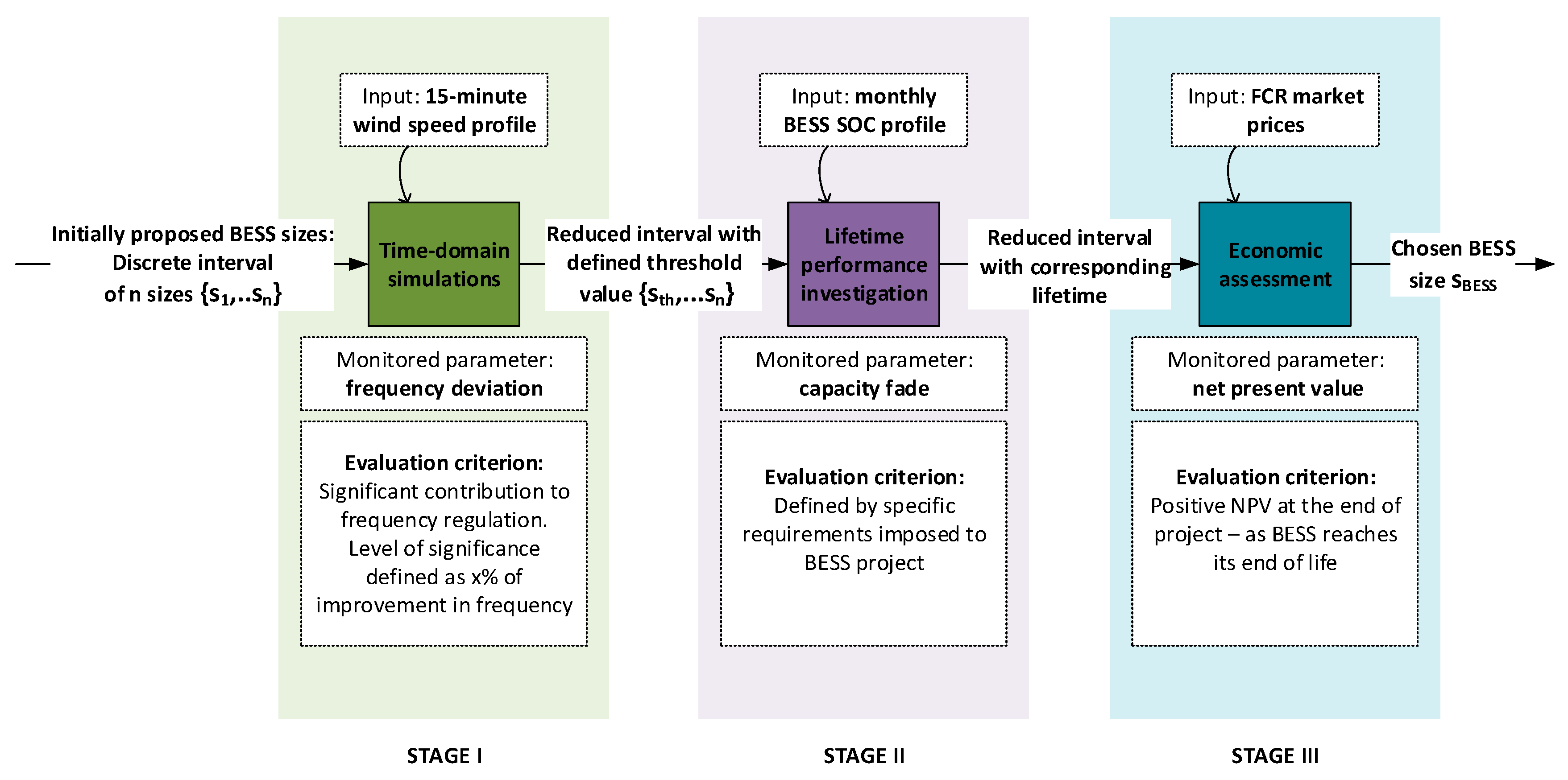
2. Sizing Methodology

The main aim of the methodology is to find the optimum BESS size by gradually reducing the initially proposed interval of BESS sizes. The initial interval is relatable to the applicable system ratings where BESS is integrated. Each reduction of the interval is the output of the assessment carried out in each stage. The reduction is determined based on the defined evaluation criteria of each stage. As marked in Figure 2, there are three main stages, each comprising of a specific type of analysis elaborated in Section 1 that is related to the BESS unit. Input parameters specific for each stage are defined, as well as a monitored parameter relatable to the evaluation criterion to be fulfilled and marked on Figure 2.

Evaluation criteria of each stage are strongly dependent on the BESS project requirements. However, the evaluation criteria marked in Figure 2 are the minimum requirements that need to be fulfilled. Additional evaluation criteria, specific to the project, can be defined in each stage. As for example, during Stage II, evaluation criteria could be defined by imposed expected BESS lifetime. For example, some projects include BESS as a part of the virtual power plant together with WT. In such cases, it could be required that the expected lifetime of the BESS unit meets the lifetime of the WT. For that purposes, the BESS performance is investigated for the period relevant to the WT lifetime [3]. During Stage II, it is then observed if the lifetime of the initially installed BESS meets the required time in service. If that is not the case, then a replacement of the BESS packs should be carried out. However, such a situation requires an additional cost, which then has to be accounted in the economic assessment of Stage III. For that purposes, specific evaluation criteria concerning the additional cost could be set. Similarly, evaluation criteria for the third stage could be defined based on the available project funding or expected profit the unit should generate. However, the main aim of defining evaluation criteria of each stage is to properly decrease the size interval and finally decide on the most suitable size fulfilling all imposed project requirements.

Additionally, to better define the evaluation criteria of each phase, prerequisite information of the system in which BESS is to be integrated is of high importance. Those are the current status and future trend of wind power capacity. By obtaining information on future WT instalments, a decision whether or not investing in larger size BESS unit than the one suitable for current system configuration should be made. Further on, information regarding current statistics on the frequency of FCR activations and an average value of frequency deviations in cases of disturbances should be collected. This is needed to have a better estimation of expected BESS operation and more accurate estimation of BESS lifetime. Finally, information relevant for the economic assessment of the BESS unit, such as a predicted instalment of other components to the system and their participation in the system frequency regulation. In order to perform the assessment study based on the proposed methodology, a suitable BESS model is created and presented in the following section.

3. System Modelling

This section outlines the developed BESS model comprising of the three modules corresponding to the different BESS aspects applicable to different parts of the proposed methodology. Those are: the performance model, the lifetime model and the economic model. In the last part of the section, the chosen benchmark power system model for the purposes of the study is introduced.

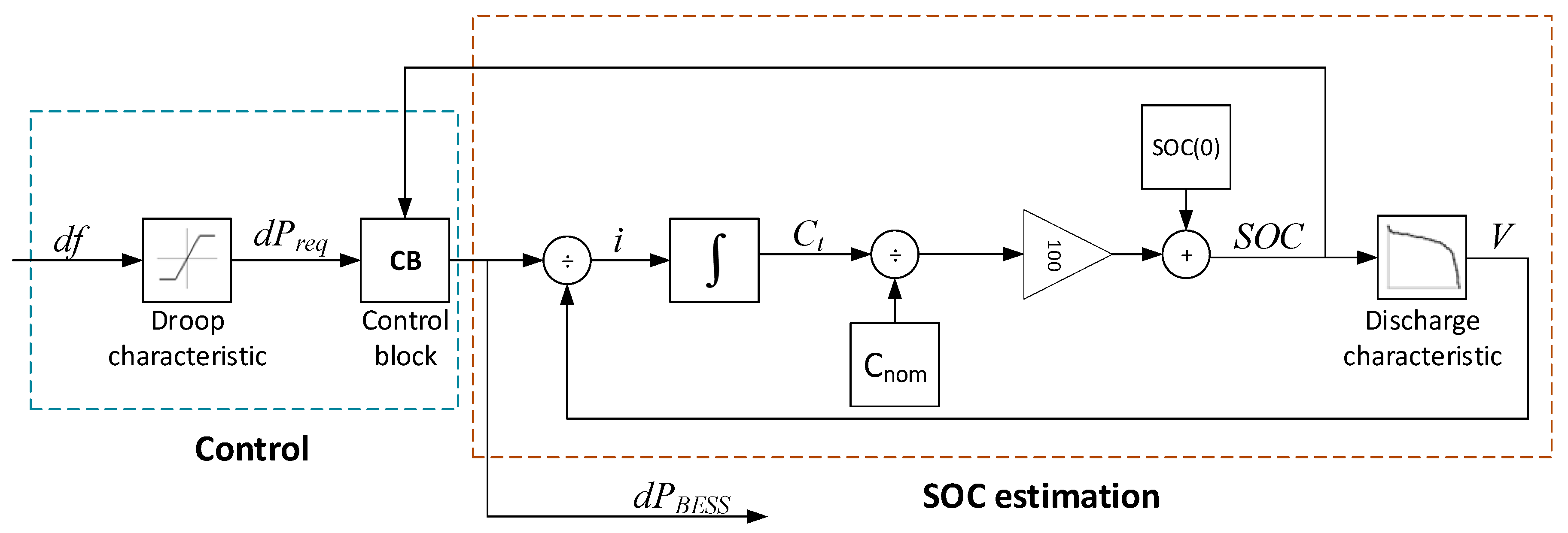
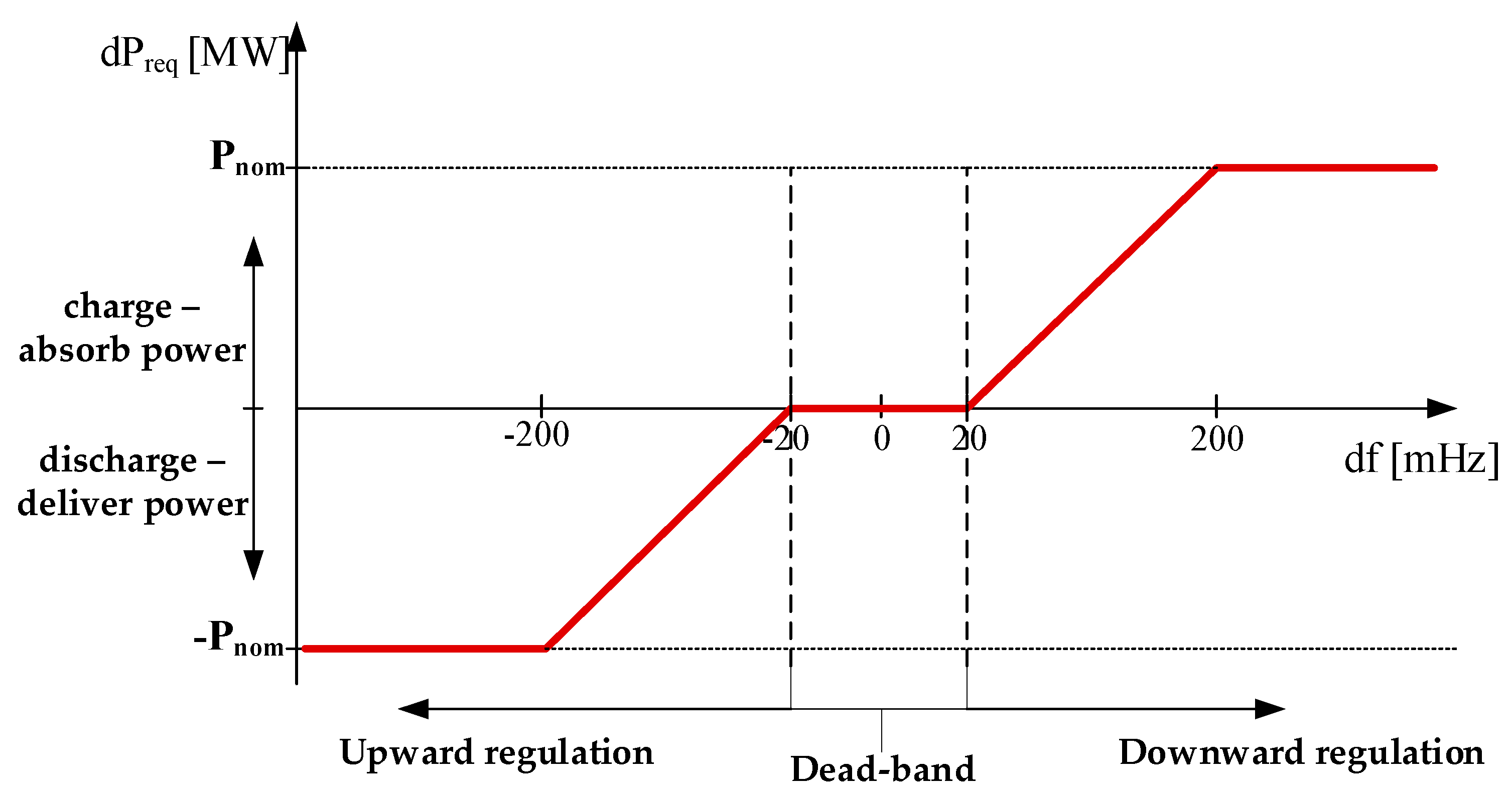
3.1. Battery Energy Storage System

3.1.1. Performance Model

The main aim of the developed performance model is to capture the BESS capability of providing FCR based on its available capacity. With that respect, the state-of-charge (SOC) is the parameter monitored during BESS operation. This parameter varies based on the amount of power that is being absorbed or delivered to the grid. Monitoring its variation gives sufficient information for the BESS response associated with the provision of FCR. The overall block diagram of the BESS performance model is shown in Figure 3. It is comprised of two main parts—the first one associated with the SOC estimation and the second one with the control part for FCR provision.

The expression describing the SOC estimation is based on the current flow through the BESS unit and it is known as the Coulomb counting method. This is the most common method used in the analysis in which BESS dynamic performance by means of SOC is being assessed. This method gives an accurate estimation of SOC [28]. Further on, a developed performance model based on the Coulomb counting method is adequate for lifetime investigation as it has included performance degradation parameters. The expression for SOC estimation is given as follows:

$$\mathrm{SOC}=SOC(0)\pm \frac{1}{C_{nom}}{\displaystyle \int i(t)dt}$$

(1)

where C_nom is the nominal capacity in Ampere hour, SOC(0) is the initial SOC value and i is the current flowing through the battery in Ampere.

The nominal capacity is the maximum available capacity of the BESS unit available at its beginning-of-life (BOL). The initial SOC value gives information on the amount of energy stored in BESS at its BOL. Depending on the type of the service BESS provides, its initial SOC can be set accordingly. For example, if BESS is only required to deliver power for a specific application, its initial SOC, as well as re-established SOC after service provision, should be 100%. In cases in which BESS is expected to both, absorb and deliver power while providing service, the most suitable initial SOC is 50%.

C_t and V are the variables in the SOC estimation part of the performance model which are not directly included in the Equation (1). C_t represents the actual available BESS capacity at the given time instant t during the BESS operation. V represents the voltage level of the BESS unit. Knowing its value is required in order to determine i, the current flowing through the BESS. The voltage level is evaluated based on the SOC level at the time instant t. SOC and V do not have a linear relationship, but their correlation is shown by the means of a standard discharge characteristic of a Li-ion BESS.

For the purpose of this research, the SOC upper and lower level are restricted to 90% and 10% respectively in order to ensure a safe and long-term operation. However, it should be pointed out that this parameter could be varied in order to examine the optimal BESS operation, which is not in the scope of this work.

The input value to the SOC estimation part of the performance model, as indicated in Figure 3, is dP_BESS representing the actual power being delivered or absorbed by BESS. This value is determined based on the grid frequency deviation df and current BESS availability represented through SOC. The control part of the model is designed in a way that it captures all imposed requirements for FCR provision. Those requirements need to be addressed when developing a suitable control strategy for any participating unit, including BESS. In Europe, there are certain countries, such as Denmark, which have developed technical regulations specific to BESS units [29]. However, those regulations comply with the imposed rules for European electricity grid. According to ENTSO-E system operation grid code [2], in case of a disturbance in the system causing frequency deviations equal to or larger than ±200 mHz:

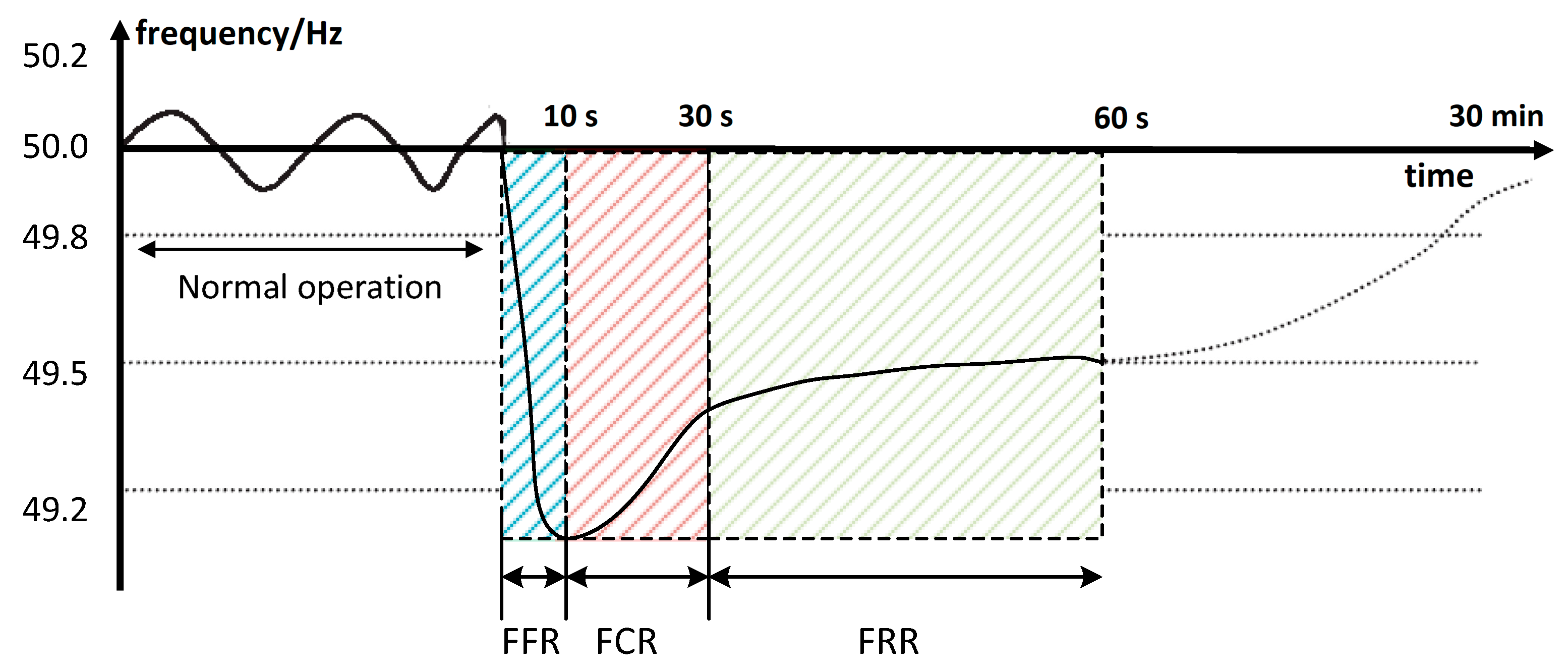
• half of the reserves need to be provided in the first 15 s after the disturbance and full activation is expected within 30 s
• participating units need to have the ability to provide the reserves for 15 min at nominal power
• participating units are entitled to 15 min re-establishing period after 15 min of reserve provision

For smaller deviations, the time requirements should be proportional to the one previously presented. The size of the units participating in the provision of FCR should be in the MW range. This is related to the specific requirements on the regulating power market. As stated in ref. [2], the minimum bid size for FCR accounts for 1 MW, while the maximum bid size for individual units equals 25 MW.

Reflecting the requirement of bringing frequency to a new steady-state after the disturbance, a proportional control is the most suitable type of control for FCR provision [30]. Reflecting its operational characteristics, the proportional controller has the ability of bringing the frequency to the new steady state. This frequency is then an input for the control system related to FRR. The proportional control for FCR is implemented by the parameter called droop which is defined as [30]:

$$R_{\%}=\frac{\Delta f_{\%}}{\Delta P_{\%}}=\frac{{\omega }_{nl}-{\omega }_{fl}}{{\omega }_0}\cdot 100\%$$

(2)

where R_% is droop value, Δf_% is change in frequency, ΔP_% is change in output power, ω_nl is the frequency at no load conditions, ω_fl is the frequency at full load conditions and ω₀ is nominal frequency.

No load conditions, when BESS should not provide or absorb any power from the grid, apply for frequency deviations within dead-band of ±20 mHz. Full load conditions, for which BESS should operate at nominal power, apply for frequency deviations equal to or larger than ±200 mHz. With that respect, droop value determined based on (2) equals 0.36% and the corresponding droop characteristic is shown in Figure 4.

Based on the droop characteristic, the actual required power that needs to be absorbed or delivered from the BESS to the grid dP_req is being determined for the input frequency deviation, df. This signal is then sent to the control block (CB) shown in Figure 3. There, it is examined if the BESS can meet the demanded power based on its current SOC. In general, a situation like that could occur if severe frequency deviations persist for more than 15 min. The output of the CB is the actual power dP_BESS that is being delivered or absorbed by BESS.

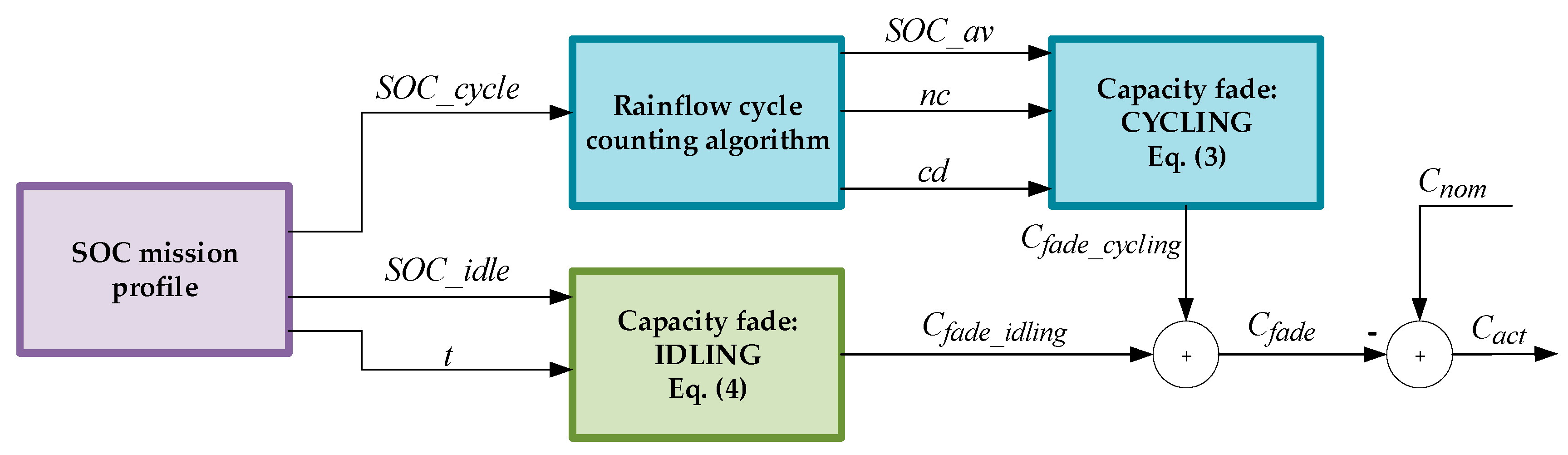
3.1.2. Lifetime Model

During BESS operation, it is necessary to monitor the stress factors and corresponding stress levels and investigate their influence on the BESS performance-degradation. In general, the stress factors are statistical parameters specific for the BESS application. They are connected to the BESS operating conditions and subsequent decrease in the lifetime. BESSs are subjected to two different operating conditions—cycling and idling. A methodology for BESS lifetime estimation during cycling and idling conditions is developed in [6]. Based on the findings in [6], it is concluded that the capacity fade is the relevant parameter for monitoring and assessment of BESS degradation. Expressions for capacity fade during cycling and idling, including parameters, are given in [19]:

$$C_{fade\_cycling}=k_1\cdot e^{a_1\cdot SOC\_av}\cdot c{d}^{b_1}\cdot n{c}^{c_1}$$

(3)

$$C_{fade\_idling}=k_2\cdot e^{a_2\cdot SOC\_l}\cdot t^{b_2}$$

(4)

where SOC_av is average SOC during one cycle in percentage, cd is cycle depth during one cycle in percentage, nc is the number of cycles, SOC_l is SOC storage level in percentage and t is storage time in months. Parameters of both equations are given in Appendix A. Equation (4) is valid for capturing capacity fade during idling for temperature equal to 25 °C. If different conditions are present, temperature influence on capacity fade has to be included, as that has been done in [6].

The main aim of developing the lifetime model is to capture the incremental loss of lifetime caused by the aforementioned operating conditions. BESS performance model presented in Section 3.1.1 has included nominal capacity, C_nom which is degrading with time. Based on the developed lifetime model, a degradation of this parameter is estimated. In that way, time-domain analysis and BESS contribution to frequency regulation can be examined with the included accurate representation of the available capacity throughout the entire time in service. The lifetime model developed for the purposes of this study is presented in Figure 5.

The input to the lifetime model is a SOC mission profile that needs to be decomposed into cycling and idling operation. The results of the decomposition are SOC_cycle and SOC_idle which contain SOC values during the aforementioned operating conditions. Additionally, information regarding the amount of time BESS spent idling at each of the SOC idling levels is attained and stored in variable t. The capacity fade during idling, C_{fade_idling} is determined by using the expression (4). In order to obtain all input parameters for Equation (3) from the SOC_cycle, the Rainflow cycle counting algorithm is used. The resulting SOC_av, cd and nc are then used in Equation (3) to obtain the capacity fade during cycling, C_{fade_cycling}. The overall capacity fade, C_fade, is the sum of the aforementioned capacity fades due to cycling and idling conditions. The output of the lifetime model is the updated capacity of the BESS unit C_act, which is decreasing as the BESS degradation evolves. Referring to the developed performance model outlined in Figure 3, C_nom is replaced by C_act after the first iteration of the capacity fade determination. C_act is then being updated after each performance degradation calculation during BESS time in service. The BESS End-of-Life (EOL) is reached when its capacity degrades to 80% of the nominal capacity C_nom [19].

The developed lifetime model requires the largest computational effort in the proposed sizing methodology. Obtaining each of the variables shown in Figure 5 is lengthy, while the Rainflow cycle counting algorithm represents the most critical part. Reduction of the computational effort can be made if an adequate time step between two consecutive capacity fade updates is chosen. Hence, too frequent capacity fade updates would result in a high simulation time and would require additional resources. However, if the time step is too large, the BESS power that is bid on the market would be larger than the actual available power. This will consequently lead to errors in the economic model. With that respect, a balance needs to be found in a way that computational effort can be as reduced as possible while at the same time the accuracy of the BESS performance is preserved.

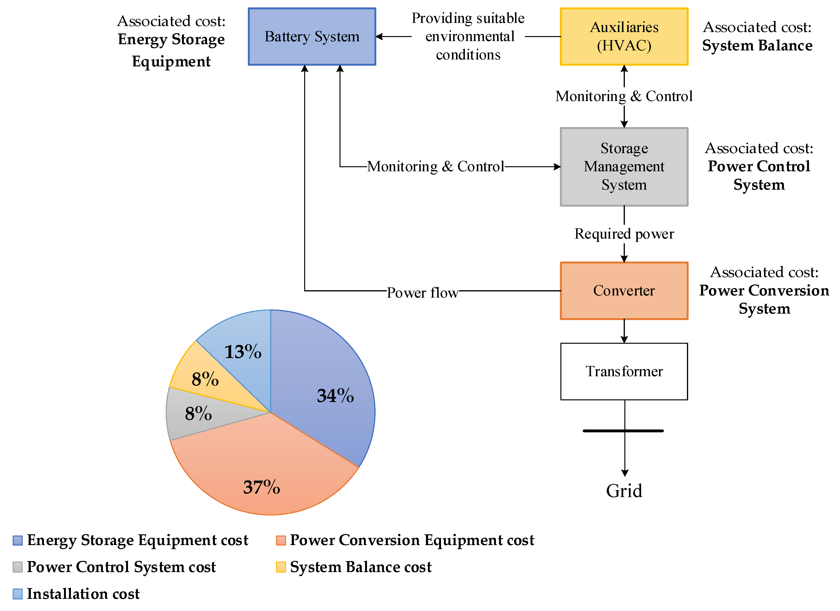
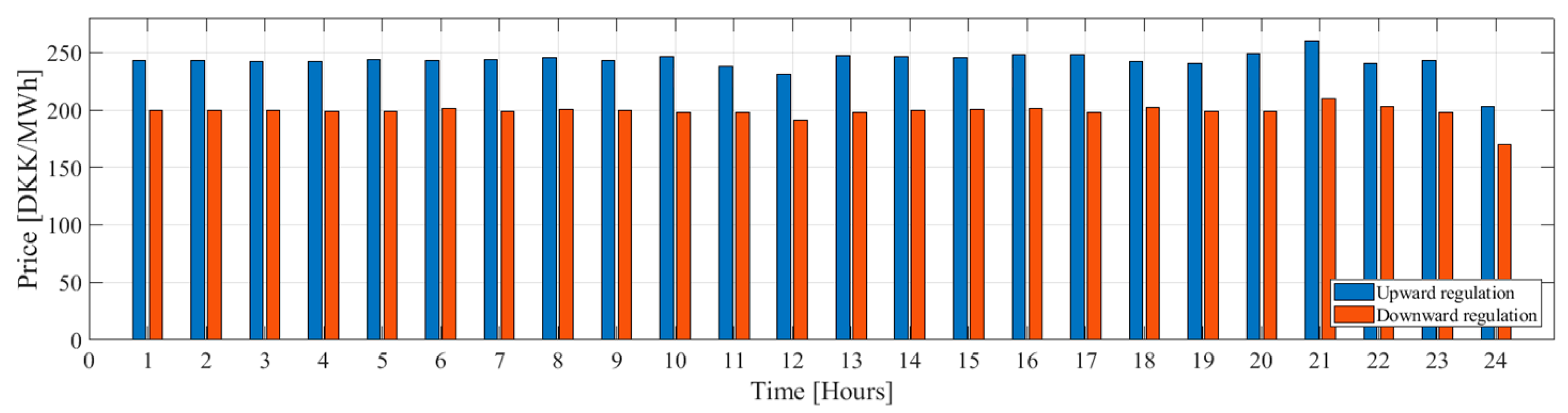
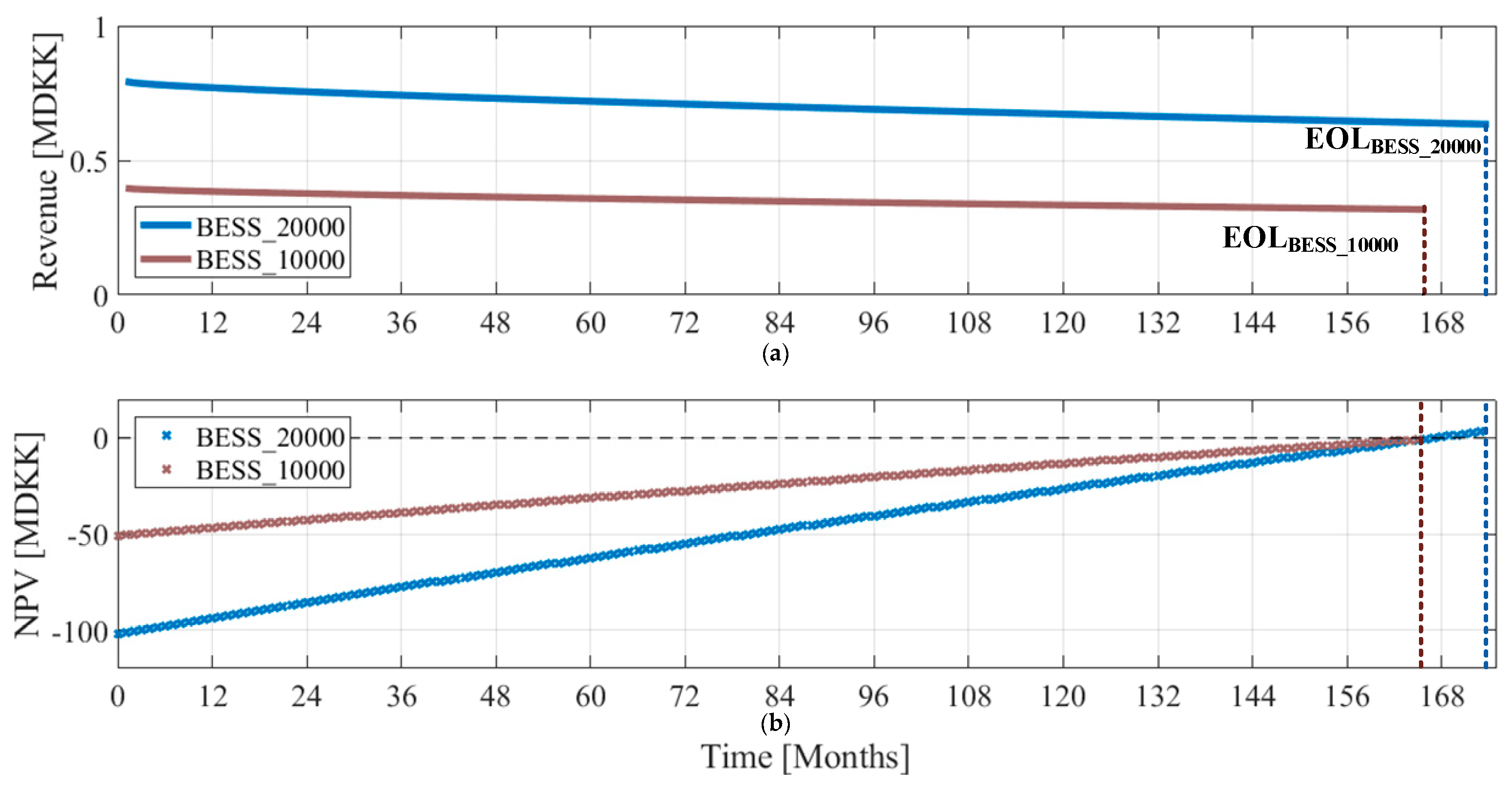
3.1.3. Economic Model

The economic model is developed with the aim of assessing the BESS’s profitability with the respect to the different storage sizes. Moreover, the influence of capacity fade on accumulated revenue can be evaluated with the developed model. In general, the suitable way of representing the BESS profit is through the Net Present Value (NPV) which is defined as:

$$NPV={\displaystyle \sum _{t=0}^{EOL}\frac{Revenue(t)-Cost(t)}{{(1+r)}^t}}$$

(5)

where Revenue represents the generated income by participating in regulating the market, Cost represents the required payment including capital and operation and maintenance (O&M) cost and r is a discount rate of the project. In this economic model, all costs are considered at the present rate, meaning that the discount rate is set to zero.

The capital cost is a fixed cost and represents the initial investment of the project. A comprehensive study on prices of energy storages, including insights from the industry, grid service providers, energy consultants and universities was carried out in [31]. Capital cost is divided into five main categories. The schematics of the BESS unit and associated costs are given in Figure 6. A distribution of the overall capital cost on five categories is also provided based on the data presented in [31].

Energy storage equipment cost represents the cost of the storage medium, which is, in this case, Li-ion packs. Furthermore, the cost of the assembling of the components into a DC system, together with internal wiring and voltage and temperature monitoring system, is accounted as well. The inverter cost is included in the power conversion system equipment cost. Power control system cost is related to the controllers used for the adequate BESS operation. This cost is specific to the application the BESS is intended to, considering that different applications have different requirements related to the BESS performance and its response. In the given example, it includes the cost of the controllers for the adequate provision of the FCR. System balance cost is including all necessary ancillary equipment for adequate BESS operational conditions, e.g., heating, ventilation and air conditioning (HVAC). As stated in [19], by keeping the operating temperature in the predefined optimal range, degradation of the BESS can be significantly decreased. Hence, investing in a HVAC system is recommended in order to assure a long lifetime. The last category includes the installation cost of the BESS unit. It represents the engineering, procurement and construction cost together with the installation of the all necessary parts. Furthermore, it includes manpower, site design, procurement and transportation of the equipment.

As shown in Figure 6, the cost of a storage unit itself represents only 34% of the capital cost. Therefore, when BESS reaches its EOL, an analysis should be performed whether it is economically beneficial to make an investment in a new storage unit or not. The rest of the listed infrastructure requires a single time initial investment.

The O&M cost is typically low for Li-ion technology. It only includes maintenance activities on the ventilation system and mechanical and electrical components. For this study, O&M cost accounts for 6 $/kW on a yearly basis [31].

Project revenue represents the generated income by participating in regulating market where bids for the provision of FCR are placed. All units participating in regulating market are paid for having extra generation capacity ready for hours for which the bids are successful regardless of their activation [25]. Therefore, in this economic model, the revenue is defined as:

$$Revenue=Reserve\times Price\times Period$$

(6)

where Reserve stands for the capacity being offered on the regulating market for the provision of FCR in MW, Price represents clearing price on the regulating market for a specific hour in DKK/MWh and Period represents the time for which the bid is placed in hours.

3.2. Benchmark Power System Model

In order to test the BESS provision of FCR in case of disturbances in the system, an adequate power grid model needs to be chosen. The system to be used for testing purposes should comprise of the conventional generating units with the implemented control strategy for the provision of FCR. Further on, load models should represent typical loads in the power grid which are, in general, frequency and voltage dependent. However, the system complexity should not be too high in order to monitor its response to the generation-demand imbalance and BESS participation in the frequency regulation. Therefore, the IEEE 14-bus system is the adequate benchmark grid model fulfilling the aforementioned requirements and is used for the testing purposes. The overall system description is provided in [32]. The relevant system specifications for the frequency stability studies are provided in Appendix A. In order to capture the BESS performance in a system dominated by renewables, an aggregated WT plant with installed capacity of 96 MW is integrated to the system. For the simplicity reasons, it is connected to the same bus as the largest conventional generating unit. The same is done with the developed model of the BESS unit.

4. Assessment Study

The main aim of the assessment study is to perform the sizing procedure by means of the proposed methodology. Graphical representations of processes relevant for each stage are shown by means of the flowcharts as presented in Figure 7.

Initialization has to be performed at the beginning of each stage. It includes common and stage-specific requirements. Common requirements are the definition of the size interval and the evaluation criteria. Definition of the initial size interval for Stage I is explained in the further part of this section. The initial size interval for the rest of the stages is based on the results of the previous analysis, as presented in Figure 2 in Section 2.

Further on, in the initialization stage, the first size in the BESS interval is integrated into the system. Stage-specific variables that are increased in each iteration are also initialized. For Stage I, that variable is a case number, which is set to the first case, and for Stage II and III, it is a month, which is set to the first month in service.

4.1. Stage I—Time-Domain Assesment

4.1.1. Initialization

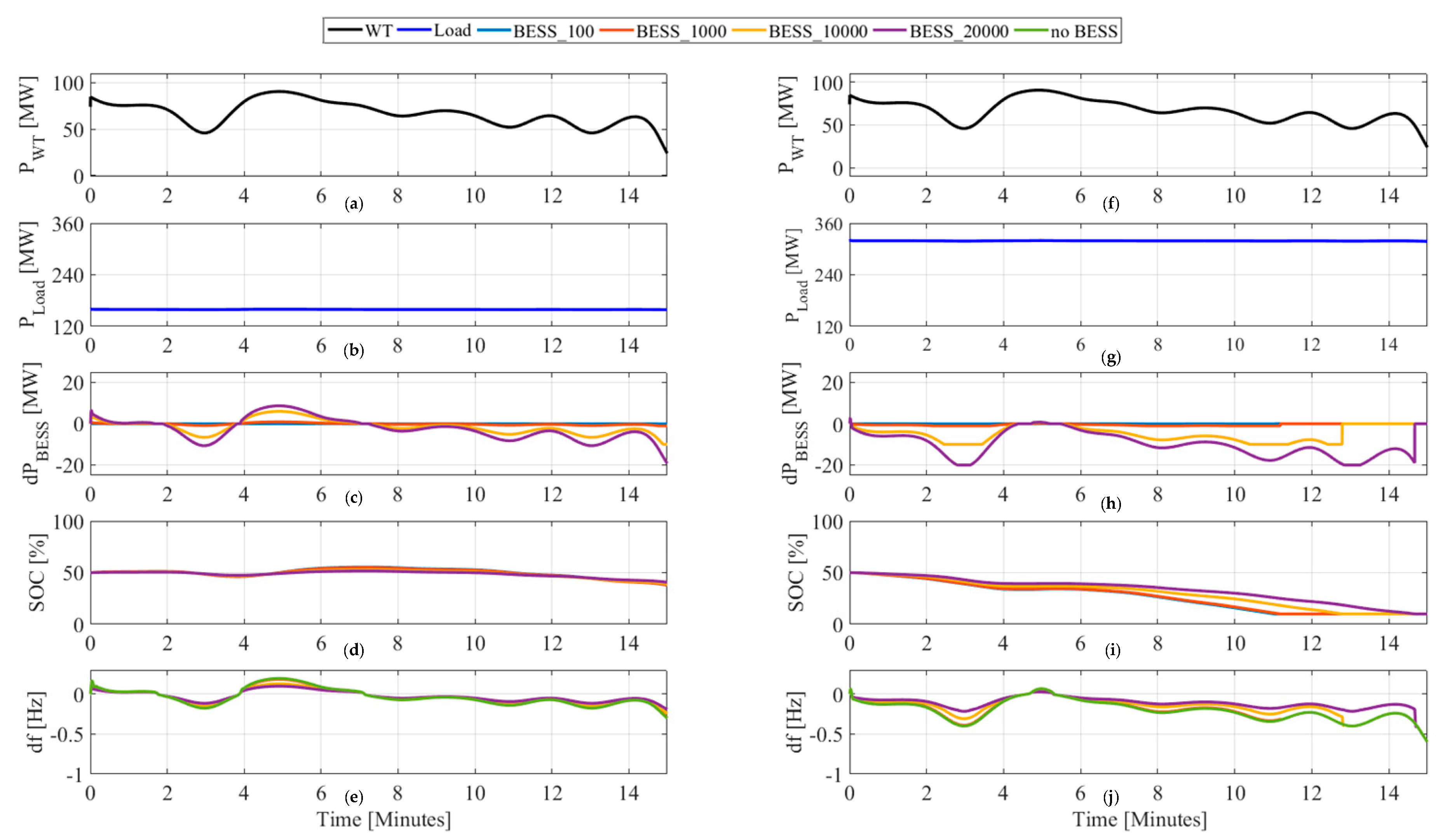
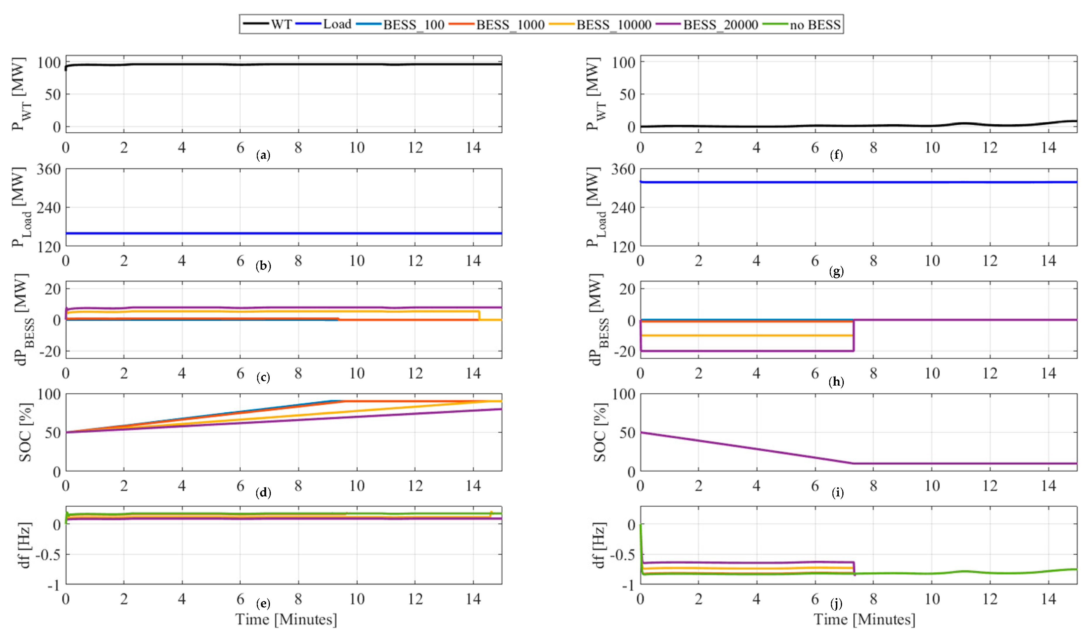
Stage-specific requirements in the initialization stage include: decision on wind power penetration level, the definition of scenarios and simulation time and choice of regulation type BESS is participating in together with adequate SOC re-establishment strategy.

In this example, it is decided that time-domain simulations are performed for 30% wind power penetration level where it is considered that the power system has entered the developed stage of wind power integration [33]. The overall active power generation in the system is subjected to fluctuations and the frequency can no longer be maintained by using conventional generating units to the same extent as before WT deployment.

Overall, four different scenarios are investigated capturing the most challenging situations for frequency stability maintenance. The scenarios are based on statistical data on wind power generation and active power demand during large frequency deviations. The overview of the scenarios is given in

Table 1. Simulation scenarios for a system with 30% wind power penetration level.

Scenario		Wind Power Generation as Percentage of 96 MW Installed Capacity	Active Power Required by the Load
First	Case I	Fluctuating Maximum: 95% Minimum: 25%	Low 160 MW or 50% of daily peak
	Case II		High 320 MW daily peak
Second		High Maximum: 100% Minimum: 95%	Low 160 MW or 50% of daily peak
Third		Low Maximum: 10% Minimum: 0%	High 320 MW daily peak

. The simulation time is set to 15 min as the required duration of the FCR provision.

The initial SOC of each unit equals 50%, as the units are participating in both upward and downward regulation. After FCR provision the SOC is re-established to 50%.

Generally, when choosing the size interval, especially the number of the initially considered sizes, certain constraints should be considered. The most relevant one is the complexity and the computational time of the each of the processes within the three stages. As the number of the initially considered sizes is increased, the computational time becomes significantly prolonged. This is especially important in Stage II of the methodology where a lifetime estimation is extremely time and resource demanding. Moreover, a decision on upper and lower BESS sizes should be based on the statistical data related to the frequency and magnitude of the disturbances in the power grid a BESS unit is implemented to. Nonetheless, a detailed guidance on the optimal choice of the initial interval of BESS sizes is proposed for future work. Additionally, the optimal difference between two consecutive BESS sizes in the initial interval will be carried out. This will be performed in order to improve the proposed methodology and its efficiency.

In this example, the initial size interval comprises of only four BESS sizes. This choice is made for the simplicity reasons and with the aim of showing the main contributions of the presented methodology. The power ratings of chosen BESS units are based on the system ratings of the generating units and demand of the studied IEEE 14 bus system. BESS_100 represents 0.1% from the 96 MW installed capacity of WTs, while BESS_20000 represents 20% of the WT installed capacity. Energy ratings are based on the 15 min requirement of FCR provision at the nominal power. The overview of the chosen BESS sizes is provided in

Table 2. Proposed initial BESS size interval.

BESS Name for Given Size	Power/Energy Rating
BESS_100	0.1 MW/0.025 MWh
BESS_1000	1 MW/0.25 MWh
BESS_10000	10 MW/2.5 MWh
BESS_20000	20 MW/5 MWh

.

There are no additional specific requirements defining evaluation criteria of this stage, except for the one elaborated in Section 2 (see Figure 2). Therefore, reduced BESS size interval, after the completion of Stage I, comprises of sizes for which contribution to the frequency regulation is significant.

4.1.2. Results

Results of the time-domain analysis are presented in Figure 8 and Figure 9. The WT power output for 15 min of simulation time is given in the Figure 8a,f and Figure 9a,f. The shown WT generation curves correspond to the suitable scenarios previously elaborated and summarized in Table 1. However, if scenarios different than the ones here presented are to be investigated, different WT power output should be attained. This is done by the means of the input wind speed profile. The variation in the input wind speed profile of the aggregated WT plant in the benchmark power system model will result in different wind power generation. This will subsequently lead to different shape and magnitude of the frequency deviation curve.

The total active power demand of the load in the benchmark power system model is shown for each scenario in the Figure 8b,g and Figure 9b,g. The active power demand of each load in the system is constant for 15 min of simulation time. This load setting is chosen as it is considered that intra hour power variations of the load are not significant. In addition, statistical, publicly available data provided by Danish Transmission System Operator on active power demand suggest the same. In [34], a 1-h resolution of data on active power demand in Denmark is available. Hence, if simulation times, longer than here selected 15 min, are considered, it is suggested that variations in active power demand are included.

Figure 8c,d,h,i and Figure 9c,d,h,i represent the BESS power output and SOC, respectively. Those are the relevant BESS parameters to be monitored in this study. Frequency deviation, as a result of the system dynamics, is shown in the Figure 8e,j and Figure 9e,j.

Based on the obtained results, it is concluded that the threshold BESS size is 10 MW/2.5 MWh. The contribution of BESS_100 and BESS_1000 to the frequency regulation is not significant. Therefore, by performing the Stage I of the proposed methodology, the input BESS size interval for the Stage II has reduced to half of the initial one. In all simulated scenarios, SOC of a smaller size unit is changed with the greater rate. The reasoning for this is found in larger frequency deviation which then requires a higher amount of regulating power to be delivered or absorbed by the BESS (as defined by droop characteristic). Out of all investigated scenarios, the frequency deviation profile obtained in the second scenario is the most probable one in a normal system operation. In general, system frequency in Continental Europe synchronous area is very close to the nominal frequency of 50 Hz. Therefore, SOC profiles of the BESS units in the second scenario are used as an input for the Stage II where the lifetime performance degradation is to be evaluated.

4.2. Stage II—Lifetime Performance Assessment

4.2.1. Initialization

A stage-specific requirement in the initialization stage includes an evaluation of the statistical data on the occurrence of FCR activation. This is necessary in order to generate a monthly SOC mission profile similar to real operation.

On the example of Lem Kær ESS providing FCR in Denmark, statistical data in [35] states that during three years of operation, the BESS performed on average 0.8 cycles per day. Hence, an assumption is made that each unit has provided FCR once per day and a SOC mission profile, as in the second scenario, is obtained. Meaning, it is assumed that large disturbance in the system has occurred which has resulted in the frequency deviation as obtained in the second scenario of the Stage I. This has resulted into the generated SOC profile for the 15 min period. It is further on assumed that 15 min FCR provision is followed by 15 min SOC re-establishment to 50% at which the unit is idling for the rest of the day. Therefore, according to the statistical data on the occurrence of the large disturbances in the system, it is further on assumed that for the rest of the day frequency deviation was within allowable dead-band of ±20 mHz.

The given one-day SOC profile is, for the purposes of this analysis extrapolated in order to obtain a monthly SOC mission profile. This mission profile is then applied as an input to the lifetime model developed in Section 3. The new capacity is updated for the faded capacity on a monthly basis and the procedure is repeated until the BESS unit reaches its EOL. The common requirement on the initial size interval of this stage is based on the simulation carried out in the previous stage. Further on, there are no specific evaluation criteria of this stage. The main aim of the lifetime investigation is to have a reduced size interval with the corresponding monthly degradation and EOL. The input interval of BESS sizes for this stage is comprising of BESS_10000 and BESS_20000.

4.2.2. Results

The capacity fade after the first month in service for BESS_10000 and BESS_20000 accounts for 0.66% and 0.62%, respectively. It increases to 3.27% and 3.12% after the first year of service. BESS_10000 reaches EOL after 166 months in service, while BESS_20000 operates for an additional eight months period. A graphical representation of the BESS capacity fade is shown in Figure 10a, while in Figure 10b, a relative difference between capacity fade of the two units is presented. As expected, the difference in capacity fade is increasing with BESS time in service. However, it should be pointed out that optimal lifetime operation has not been investigated. The main emphasis has been put on investigating how BESSs of different sizes degrade with their time in service when subjected to the same grid conditions. Investigations of the optimal idling SOC, recharging strategy, SOC limits and other relevant parameters are proposed as future work.

Since there are no specific requirements imposed for the units in service such as minimum required lifetime due to the specific project requirements, in this example the size interval is not reduced. However, an important information regarding expected time in service and monthly degradation behaviour caused by daily FCR provision of each unit is obtained. That information will be taken into account when choosing the final size after the economic analysis is performed in stage III.

4.3. Stage III—Economic Assessment

4.3.1. Initialization

A stage-specific requirement in the initialization stage includes the definition of the achieved clearing prices on the regulating market.

In this analysis, FCR prices from 2017 achieved on Nord Pool, a common Nordic electricity market that operates in Denmark, are considered and represented in Figure 11 [36]. Hourly prices of both upward and downward regulating power for one day are the average of the yearly prices for the given hour of the day.

It is further on assumed that all bids are successful and that each unit is bidding on the market for the maximum available time, which accounts for 12 h in a day (the rest of the day is allocated for re-establishing period). However, units participating in this type of regulation are paid for having extra power generation ready and not when FCR is actually activated. Therefore, FCR is activated only once per day, while all bids for 12-h time period are successful and contribute to the generated revenue.

Evaluation criteria of this stage are defined in Section 2 (see Figure 2) and no additional specific requirements should be considered. Therefore, the final BESS size is determined based on the requirement of positive NPV as BESS EOL is reached. However, a case of more than one BESS size fulfilling all the defined criteria could occur. An outcome of the sizing procedure is then an interval of final BESS sizes, instead of one specific BESS size. In that case, the choice of the final BESS size should be based on current and future trends of wind power integration (as elaborated in Section 2). Nonetheless, it is assured that the final chosen size is fulfilling all the imposed criteria.

4.3.2. Results

As indicated in the flowchart presented in Figure 7, by using the developed economic model presented in Section 3, the project NPV is evaluated on a monthly basis. The available regulating power determined in Stage II is considered in the evaluation process. The results of the economic analysis are illustrated in Figure 12. As expected, revenues are gradually decreasing with the BESS time in service. This is due to the capacity fade and subsequently reduced available regulating power. BESS_10000 attains its EOL before reaching the payback time. Hence, the NPV of BESS_10000 is negative. The NPV of BESS_20000 is positive and accounts for 3 million DKK, while its payback time equals 14 years. The percentage of the final profit in the initial investment equals −1.63% and 3.10% for BESS_10000 and BESS_20000 respectively.

The evaluation criterion for Stage III, i.e., positive NPV at the EOL, is not fulfilled by BESS_10000. Therefore, the chosen BESS size is 20 MW/5 MWh. In addition, it is expected that the wind power penetration level will increase in the future, which is a supporting fact for investing in the integration of BESS_20000.

In the presented example, the largest size of all considered is the suitable one. Additional analysis could be carried out in order to determine if larger size units would fulfil all imposed criteria as well. As stated in Section 4.1.1, the initial interval of BESS sizes is based on the benchmark power system ratings. Larger sizes were not taken into account in the given example as it is considered that BESS capacity would not be utilized to a high extent—the BESS unit would be oversized for the current system setup. This means that the result of the time-domain analysis would show that BESS capacity is too big for the given application and BESS would idle most of its time in service. Furthermore, in order to properly investigate the suitability of the BESS sizes close to the chosen one, additional evaluation criteria should be defined. However, the authors of the paper only relayed on publicly available data on the similar BESS project in the given example. In such cases, the lack of necessary information represented an obstacle to define additional evaluation criteria. Nonetheless, the given example only served to illustrate the benefits of the proposed sizing methodology.

5. Conclusions

This paper has presented a methodology for the determination of the suitable BESS size providing system stability services in a wind-dominated power system. The main aim of the proposed methodology is to perform the sizing procedure by continuously decreasing the initially proposed BESS size interval. The decrease is conducted based on the imposed criteria to be fulfilled involving different BESS performance aspects. For that purpose, the suitable BESS model is developed comprising of the three different modules—performance, lifetime and economic. The studied example reveals that a decision based only on one type of analysis would not result in the choice of the suitable BESS size due to insufficient information. BESS_10000 would be a suitable choice if a decision was based on results obtained only by performing time-domain simulations and lifetime performance investigation. However, it has been shown that this unit reaches its EOL before the payback time of the project is reached.

Further on, with the proposed methodology, a wide variety of system operation scenarios can be tested and resulting BESS behaviour can be analysed. Subsequently, this will lead to the less unpredictable BESS operation within its time in service. Moreover, a clear understanding of BESS degradation and related economic profitability will be obtained. Hence, the proposed methodology and its developed models can be used, “as-it-is”, by system engineers in the planning stage as well as system operators during BESS operation.

In the studied example, the wind power penetration level has been set fixed to 30%. Accordingly, the simulations have been performed for a fixed WT installed capacity throughout the entire sizing methodology. In the case of an increased WT installed capacity, additional simulations can be performed to investigate the BESS performance. The developed models can be used to assess the BESS dynamic and degradation behaviour in scenarios with higher wind power penetration scenarios even after the suitable size is chosen.

Finally, sizing methodology can be adjusted for sizing BESS unit providing other types of services than here considered FCR.

Future work is addressed for further testing of the hereby presented sizing methodology. It includes activities already being in progress, such as the integration of the developed control system for Real-Time Hardware-In-the-Loop testing. The main aim is to test BESS performance in conditions closer to the real system operation. This is intended to be done by means of laboratory facilities at Aalborg University.

References

1. REN21 Renewables. Global Status Report. 2018. Available online: http://www.ren21.net/wp-content/uploads/2018/06/17-8652_GSR2018_FullReport_web_final_.pdf (accessed on 7 August 2018).
2. European Commission COMMISSION REGULATION (EU) 2017/1485—of 2 August 2017—Establishing a Guideline on Electricity Transmission System Operation. Available online: http://eur-lex.europa.eu/legal-content/EN/TXT/PDF/?uri=CELEX:32017R1485&from=EN (accessed on 7 August 2018).
3. Swierczynski, M.; Stroe, D.; Teodorescu, R.; Stan, A.I. Primary Frequency Regulation with Li-ion Battery Energy Storage System: A Case Study for Denmark. In Proceedings of the IEEE ECCE Asia Downunder, Melbourne, Australia, 3–6 June 2013; pp. 487–492. [Google Scholar]
4. Kjar, P.C.; Larke, R. Experience with primary reserve supplied from energy storage system. In Proceedings of the 17th European Conference on Power Electronics and Applications, EPE-ECCE Europe, Geneva, Switzerland, 8–10 September 2015; pp. 1–6. [Google Scholar]
5. World Energy Council World Energy Resources E-Storage 2016. Available online: https://www.worldenergy.org/wp-content/uploads/2017/03/WEResources_E-storage_2016.pdf (accessed on 20 May 2018).
6. Stroe, D.; Swierczynski, M.; Stan, A.; Teodorescu, R. Accelerated Lifetime Testing Methodology for Lifetime Estimation of Lithium-ion Batteries used in Augmented Wind Power Plants. IEEE Trans. Ind. Appl. 2014, 50, 690–698. [Google Scholar] [CrossRef]
7. Liu, X.; Wang, P.; Loh, P.C. A hybrid AC/DC microgrid and its coordination control. IEEE Trans. Smart Grid 2011, 2, 278–286. [Google Scholar]
8. Xu, L.; Chen, D. Control and operation of a DC microgrid with variable generation and energy storage. IEEE Trans. Power Deliv. 2011, 26, 2513–2522. [Google Scholar] [CrossRef]
9. Shi, W.; Xie, X.; Chu, C.C.; Gadh, R. Distributed Optimal Energy Management in Microgrids. IEEE Trans. Smart Grid 2015, 6, 1137–1146. [Google Scholar] [CrossRef]
10. Chen, S.X.; Gooi, H.B.; Wang, M.Q. Sizing of energy storage for microgrids. IEEE Trans. Smart Grid 2012, 3, 142–151. [Google Scholar] [CrossRef]
11. Chaouachi, A.; Kamel, R.M.; Andoulsi, R.; Nagasaka, K. Multiobjective Intelligent Energy Management for a Microgrid—Aymen Chaouachi—Academia. IEEE Trans. Ind. Electron. 2013, 60, 1688–1699. [Google Scholar] [CrossRef]
12. Liu, H.; Hu, Z.; Song, Y.; Wang, J.; Xie, X. Vehicle-to-Grid Control for Supplementary Frequency Regulation Considering Charging Demands. IEEE Trans. Power Syst. 2015, 30, 3110–3119. [Google Scholar] [CrossRef]
13. Han, S.; Soo, H.H.; Sezaki, K. Design of an optimal aggregator for vehicle-to-grid regulation service. In Proceedings of the 2010 Innovative Smart Grid Technologies (ISGT), Gothenburg, Sweden, 19–21 January 2010. [Google Scholar]
14. He, Y.; Venkatesh, B.; Guan, L. Optimal scheduling for charging and discharging of electric vehicles. IEEE Trans. Smart Grid 2012, 3, 1095–1105. [Google Scholar] [CrossRef]
15. Yilmaz, M.; Krein, P.T. Review of the impact of vehicle-to-grid technologies on distribution systems and utility interfaces. IEEE Trans. Power Electron. 2013, 28, 5673–5689. [Google Scholar] [CrossRef]
16. Li, X.; Huang, Y.; Huang, J.; Tan, S.; Wang, M.; Xu, T.; Cheng, X. Modeling and control strategy of battery energy storage system for primary frequency regulation. In Proceedings of the International Conference on Power System Technology, Chengdu, China, 20–22 October 2014; pp. 543–549. [Google Scholar]
17. Knap, V.; Chaudhary, S.K.; Stroe, D.; Swierczynski, M.; Craciun, B.; Teodorescu, R. Sizing of an Energy Storage System for Grid Inertial Response and Primary Frequency Reserve. Trans. Power Syst. 2016, 31, 3447–3456. [Google Scholar] [CrossRef]
18. Benato, R.; Dambone Sessa, S.; Musio, M.; Palone, F.; Polito, R. Italian Experience on Electrical Storage Ageing for Primary Frequency Regulation. Energies 2018, 11, 2087. [Google Scholar] [CrossRef]
19. Stroe, D.; Swierczynski, M.; Stroe, A.; Member, S.; Laerke, R.; Kjaer, P.C.; Member, S.; Teodorescu, R. Degradation Behavior of Lithium-Ion Batteries Based on Lifetime Models and Field Measured Frequency Regulation Mission Profile. IEEE Trans. Ind. Appl. 2016, 52, 5009–5018. [Google Scholar] [CrossRef]
20. Stroe, D.I.; Knap, V.; Swierczynski, M.; Stroe, A.I.; Teodorescu, R. Operation of a grid-connected lithium-ion battery energy storage system for primary frequency regulation: A battery lifetime perspective. IEEE Trans. Ind. Appl. 2017, 53, 430–438. [Google Scholar] [CrossRef]
21. Gatta, F.; Geri, A.; Lamedica, R.; Lauria, S.; Maccioni, M.; Palone, F.; Rebolini, M.; Ruvio, A. Application of a LiFePO4 Battery Energy Storage System to Primary Frequency Control: Simulations and Experimental Results. Energies 2016, 9, 887. [Google Scholar] [CrossRef]
22. Jozef, M.; Thorbergsson, E.; Knap, V.; Swierczynski, M.; Stroe, D.; Teodorescu, R. Primary Frequency Regulation with Li-Ion Battery Based Energy Storage System—Evaluation and Comparison of Different Control Strategies. In Proceedings of the Intelec 2013, 35th International Telecommunications Energy Conference, Hamburg, Germany, 13–17 October 2013; pp. 1–6. [Google Scholar]
23. Mercier, P.; Cherkaoui, R.; Member, S.; Oudalov, A. Optimizing a Battery Energy Storage System for Frequency Control Application in an Isolated Power System. IEEE Trans. Power Syst. 2009, 24, 1469–1477. [Google Scholar] [CrossRef]
24. Brekken, T.K.A.; Yokochi, A.; Von Jouanne, A.; Yen, Z.Z.; Hapke, H.M.; Halamay, D.A.; Member, S. Optimal Energy Storage Sizing and Control for Wind Power Applications. Trans. Power Syst. 2011, 2, 69–77. [Google Scholar] [CrossRef]
25. Oudalov, A.; Chartouni, D.; Ohler, C. Optimizing a Battery Energy Storage System for Primary Frequency Control. IEEE Trans. Power Syst. 2007, 22, 1259–1266. [Google Scholar] [CrossRef]
26. Bignucolo, F.; Caldon, R.; Coppo, M.; Pasut, F.; Pettinà, M. Integration of lithium-ion battery storage systems in hydroelectric plants for supplying primary control reserve. Energies 2017, 10, 98. [Google Scholar] [CrossRef]
27. Bignucolo, F.; Caldon, R.; Pettinà, M.; Pasut, F. Renewables contributing to Primary Control Reserve: The role of Battery Energy Storage Systems. In Proceedings of the 17th IEEE International Conference on Environment and Electrical Engineering and 2017 1st IEEE Industrial and Commercial Power Systems Europe, EEEIC/I and CPS Europe, Milan, Italy, 6–9 June 2017; pp. 1–6. [Google Scholar]
28. Pillai, J.R.; Bak-Jensen, B. Integration of vehicle-to-grid in the Western Danish power system. IEEE Trans. Sustain. Energy 2011, 2, 12–19. [Google Scholar] [CrossRef]
29. Technical Regulation 3.3.1 for Battery Plants. Available online: https://en.energinet.dk/Electricity/Rules-and-Regulations/Regulations-for-grid-connection (accessed on 20 April 2018).
30. Kundur, P. Power System Stability and Control; McGraw-Hill: New York, NY, USA, 1994. [Google Scholar]
31. KEMA Inc. Battery Energy Storage Study for the 2017. Available online: http://www.pacificorp.com/content/dam/pacificorp/doc/Energy_Sources/Integrated_Resource_Plan/2017_IRP/10018304_R-01-D_PacifiCorp_Battery_Energy_Storage_Study.pdf (accessed on 20 May 2018).
32. Illinois Center for a Smarter Electric Grid (ICSEG) IEEE 14-bus System. Available online: http://icseg.iti.illinois.edu/ieee-14-bus-system/ (accessed on 20 April 2018).
33. Altin, M.; Teodorescu, R.; Jensen, B.B.; Annakkage, U.D.; Iov, F.; Kjaer, P.C. Methodology for assessment of inertial response from wind power plants. In Proceedings of the IEEE Power and Energy Society General Meeting, San Diego, CA, USA, 22–26 July 2012; pp. 1–8. [Google Scholar]
34. Energinet Data Service. Available online: https://www.energidataservice.dk/en/ (accessed on 1 October 2018).
35. Danish Technological Institute BESS project—Smart Grid Ready Battery Energy Storage System for Future Grid. Available online: https://energiforskning.dk/sites/energiteknologi.dk/files/slutrapporter/bess_final_report_forskel_10731.pdf (accessed on 16 May 2018).
36. NordPool Historical Market Data. Available online: https://www.nordpoolgroup.com/historical-market-data/ (accessed on 20 May 2018).
Figure 1. Frequency regulation processes and their activation times.
Energies 11 03065 g001
Figure 2. Three-stage sizing methodology for determination of the optimal BESS size.
Energies 11 03065 g002
Figure 3. Block diagram of BESS performance model.
Energies 11 03065 g003
Figure 4. Droop characteristic of BESS unit participating in the provision of FCR.
Energies 11 03065 g004
Figure 5. Developed lifetime model of the BESS unit.
Energies 11 03065 g005
Figure 6. Schematics of BESS and distribution of associated capital costs categories.
Energies 11 03065 g006
Figure 7. Flowchart of each stage of the proposed methodology.
Energies 11 03065 g007
Figure 8. Simulation results for First scenario: Case I (ae), Case II (fj).
Energies 11 03065 g008
Figure 9. Simulation results for: Second scenario (ae), Third scenario (fj).
Energies 11 03065 g009
Figure 10. (a) Capacity fade for reduced interval of BESS sizes, (b) Relative difference of capacity fade with the referent capacity of BESS_20000.
Energies 11 03065 g010
Figure 11. Hourly FCR prices for upward and downward regulation.
Energies 11 03065 g011
Figure 12. Results of the economic analysis: (a) Revenue, (b) NPV.
Energies 11 03065 g012