Wind Turbine Multi-Fault Detection and Classification Based on SCADA Data

Abstract

Due to the increasing installation of wind turbines in remote locations, both onshore and offshore, advanced fault detection and classification strategies have become crucial to accomplish the required levels of reliability and availability. In this work, without using specific tailored devices for condition monitoring but only increasing the sampling frequency in the already available (in all commercial wind turbines) sensors of the Supervisory Control and Data Acquisition (SCADA) system, a data-driven multi-fault detection and classification strategy is developed. An advanced wind turbine benchmark is used. The wind turbine we consider is subject to different types of faults on actuators and sensors. The main challenges of the wind turbine fault detection lie in their non-linearity, unknown disturbances, and significant measurement noise at each sensor. First, the SCADA measurements are pre-processed by group scaling and feature transformation (from the original high-dimensional feature space to a new space with reduced dimensionality) based on multiway principal component analysis through sample-wise unfolding. Then, 10-fold cross-validation support vector machines-based classification is applied. In this work, support vector machines were used as a first choice for fault detection as they have proven their robustness for some particular faults, but at the same time have never accomplished the detection and classification of all the proposed faults considered in this work. To this end, the choice of the features as well as the selection of data are of primary importance. Simulation results showed that all studied faults were detected and classified with an overall accuracy of 98.2%. Finally, it is noteworthy that the prediction speed allows this strategy to be deployed for online (real-time) condition monitoring in wind turbines.

1. Introduction

Wind energy offers many advantages, as it is an inexhaustible clean fuel source. This explains why it is one of the fastest-growing renewable sources against greenhouse effects. Currently, research efforts are aimed at minimizing the overall cost of this energy. The tendency to use larger wind turbines (WTs) in harsh operating environments (e.g., offshore) implies that one of the main cost drivers is directly related to operation and maintenance actions. Thus, fault diagnosis (FD) is crucial for wind power to be cost-competitive, and even more so for offshore wind farms where bad weather conditions (e.g., storms, high tides, etc.) can prevent any repair actions for several weeks.

A variety of surveys on FD considering different WT components have recently been published. For example, in [1] a wide variety of WT fault locations are considered—rotor, gearbox, bearing, main shaft, hydraulic system, tower, generator, and sensors—as well as the different signal processing methods that are most frequently used in the literature to deal with these types of faults. Reference [2] mainly aims to survey the most recent condition and performance monitoring approaches of WTs with the primary focus on blade, gearbox, generator, braking system, and rotor. However, the more recent trend in this type of literature review is to focus on a specific WT sub-assembly: the bearings and planetary gearbox [3,4], the generator and power converter [5,6], the blades [7,8], etc. Most of these methods, which focus on a specific part of the WT, require the choice of the most appropriate sensors, their advisable position in the sub-assembly, and the most convenient strategy to extract as much information as possible from the obtained data. These are highly localized strategies, and each one relies on the installation of (costly) extra sensors. However, it should be possible to retrofit a multi-fault condition monitoring package onto existing WTs without requiring additional sensors and wiring on the machines. In fact, there is a large amount of operational (Supervisory Control and Data Acquisition—SCADA) data available (already collected at the WT controller), which can be used to diagnose the turbine condition. This section addresses the state-of-the-art in the FD of WT faults using SCADA data.

In recent years, there have been efforts to develop FD strategies by analyzing only SCADA data. The use of machine learning techniques has been crucial in this area. For example, in [9], fault prediction and diagnosis for the WT generator is accomplished using real-world SCADA data from two wind power plants located in China based on principal component analysis (PCA) and unsupervised clustering methods. In [10], a FD strategy for WT gearboxes is proposed based on artificial neural networks (ANNs) and tested on real-world SCADA data sets of a wind farm in Southern Italy. In [11], a strategy to diagnose WT faults from SCADA data using support vector machines (SVMs) is advised. Generally, the classification methods that deserve special mention are SVM and ANN, because of their ability to handle non-linear and noisy data. On one hand, the use of ANNs has drawbacks related to their training time and dependability on the optimization of fine-tuning their parameters. In particular, in [12] the correct number of parameters and their corresponding values must be carefully selected to create a normal behavior model based on an ANN. On the other hand, the SVM is simpler and has successfully proven its suitability in this type of problem. Thus, the SVM is the selected classifier in this paper.

Considerable research has been done on FD methods based on SVM classifiers that analyze only SCADA data. For example, different faults are studied in [13], but faults in the pitch actuators unfortunately could not be detected, and furthermore, the sampling period is unfeasible ($0.01$ s). Note that SCADA data is typically recorded at 10-min intervals to reduce transmitted data bandwidth and storage. In [14], an SVM could isolate some faults, except for high varying dynamics (including a pitch actuator fault), where the use of an observer, which is model-based, was found necessary and, again, the sampling period was $0.01$ s. Later references based on SVM are, mainly, specifically tailored for a particular type of fault. For example, in [15] an SVM-based method is proposed to classify the misalignment type of fault; generator faults are diagnosed in [9]; only actuator faults are considered in [16]; and generator and power feeder cables faults are diagnosed in [11]. In this paper, we widen the number and type of the studied faults with a unique strategy to cope with them all: three different pitch actuator faults (i.e., high air content in oil, pump wear, hydraulic leakage), a generator speed sensor fault (gain factor of $1.2$), three different pitch sensor faults (stuck in 5 deg, stuck in 10 deg, and with a gain factor of $1.2$), and a torque actuator offset fault.

As has been noted previously, one of the major drawbacks to using SCADA data is the 10-minute sampling period. This low-frequency resolution negatively affects the diagnosis capabilities, and may hide short-lived events. On the other hand, high-resolution (but feasible) SCADA data should allow the dynamic turbine behavior to be identified with higher fidelity and thus improve detection efficiency. As stated in [17,18], in this work a research framework is proposed that takes SCADA data with an additional high but feasible (1 s) frequency from the sensors. That is, the only requirement is to increase the frequency rate in the SCADA data from the already available sensors. Following this idea, in this work, we propose a strategy to detect and classify (through SVM) multiple WT faults using only conventional SCADA data with an additional, but feasible (sampling period of 1 s), high-frequency sampling from the sensors and without the added cost of retrofitting additional sensors to the turbine.

This paper is organized as follows. In Section 2, the WT benchmark model is introduced and the proposed FD strategy is described. The obtained results are presented and discussed in Section 3. Section 4 states the conclusions and future work.

2. Fault Diagnosis Strategy

2.1. Model Overview

As mentioned in the introduction, the utmost importance of WT fault diagnosis stimulated the proposal of a model, given in Reference [19], encompassing the prevailing faults encountered in practice. This early version of the model described a generic 4.8 MW three-blade horizontal-axis variable-speed WT, and it was issued by the company KK Wind Solutions [20] together with MathWorks, Inc. [21] and Aalborg University to release an international competition on fault detection and isolation in WTs. Several teams participated in the contest, and five of the solutions are compared in [22]. A second enhanced model was presented in [23] that incorporated a more realistic WT simulated using the FAST software (National Renewable Energy Laboratory, Golden, Colorado, USA). This is an aeroelastic WT simulator designed by the U.S. National Renewable Energy Laboratory’s (NREL) National Wind Technology Center and is widely used by the research community. Several FAST models of WTs of varying sizes are available in the public domain, including NREL’s 5 MW baseline turbine, which is the one used by the model. It is noteworthy that this simulator is able to consider the WT flexible modes that are present in practice, making fault detection more difficult compared to simpler models neglecting these modes (as in [19]). Thus, the second enhanced model, stated in [23], is the one utilized in this work.

The model proposes to simulate the sensors in the block diagram environment Simulink by adding signals from band-limited white noise blocks that are parameterized by noise power to the actual variables provided by the FAST software. These random noise blocks represent measurement noise either due to electrical noise in the system or due to the measuring principle. The different sensors provided in the model are shown in

Table 1. Available sensors (measured data).

Number	Sensor Type	Symbol	Unit	Noise Power
S1	Generated electrical power	$P_{e,m}$	W	10
S2	Rotor speed	${\omega }_{r,m}$	rad/s	${10}^{-4}$
S3	Generator speed	${\omega }_{g,m}$	rad/s	$2·{10}^{-4}$
S4	Generator torque	${\tau }_{c,m}$	Nm	$0.9$
S5	Pitch angle of first blade	${\beta }_{1,m}$	deg	$1.5·{10}^{-3}$
S6	Pitch angle of second blade	${\beta }_{2,m}$	deg	$1.5·{10}^{-3}$
S7	Pitch angle of third blade	${\beta }_{3,m}$	deg	$1.5·{10}^{-3}$
S8	Tower top fore-aft acceleration	$a_{fa,m}$	m/s2	$5·{10}^{-4}$
S9	Tower top side-to-side acceleration	$a_{ss,m}$	m/s2	$5·{10}^{-4}$

with the measurement noise modeled as a Gaussian white noise. Finally, a sampling period of $0.0125$ s is used in the simulations.

The most important features of the WT are detailed in

Table 2. Gross properties of the wind turbine.

Reference Wind Turbine	Data
Rated power	5 MW
Number of blades	3
Rotor/Hub diameter	126 m, 3 m
Hub height	90 m
Cut-in, rated, cut-out wind speed	3 m/s, 11.4 m/s, 25 m/s
Rated generator speed (${\omega }_{ng}$)	1173.7 rpm
Gearbox ratio	97

. In this paper, we deal with the full load region of operation in the sense that the proposed controller main objective is that the electric power closely follows the rated power.

A set of fault scenarios are defined in the WT model. These scenarios are primarily introduced in sensors and actuators. More precisely, the types of faults are gain factors, offsets, changes in the system dynamics, and stuck, as shown in

Table 3. Fault scenarios.

Number	Fault	Type
F1	Pitch actuator—High air content in oil	Change in system dynamics
F2	Pitch actuator—Pump wear	Change in system dynamics
F3	Pitch actuator—Hydraulic leakage	Change in system dynamics
F4	Generator speed sensor	Gain factor (1.2)
F5	Pitch sensor	Stuck value (${\beta }_{3,m}=5$ deg)
F6	Pitch sensor	Stuck value (${\beta }_{3,m}=10$ deg)
F7	Pitch sensor	Gain factor (1.2)
F8	Torque actuator	Offset value (2000 Nm)

. These faults are inspired by research in both proprietary and public domain sources [23]. As an extra reference, the interested reader can find a comprehensive description of these faults and their importance in [24].

The stochastic, full-field, turbulent-wind simulator TurbSim—developed by NREL—was used to generate the wind velocity fields applied in the simulations. It employs a stochastic model—as opposed to a physics-based model—to numerically simulate time series of three-component wind-speed vectors. It provides the ability to drive simulations of complex turbine designs with realistic but simulated inflow turbulence environments that combine many of the main fluid dynamic features known to negatively affect turbine aeroelastic response and loading. In this work, the generated wind data had the following features: Kaimal turbulence model with intensity set to 10%, mean speed set to $18.2$ m/s and simulated at hub height, logarithmic profile wind type, and the roughness factor was set to $0.01$ m. In this work, each simulation was run with a different wind data set. More precisely, 260 different wind data sets of a duration of 600 s each were used.

2.2. Noise Handling

To deal with noise in a data set, two broad ways can be considered, in general: (i) it can be filtered out; or (ii) left as it is. Obviously, pros and cons appear when adopting any either of these approaches. By filtering out the noisy instances from the data, there is a trade-off between the amount of information available for building the classifier and the amount of noise retained in the data set. Robust algorithms do not require preprocessing of the data—the data set is taken as is, with the noisy instances—but a classifier built from a noisy data set may be less predictive and its representation may be less compact than it could have been if the data were not noisy. The second approach was used in this work. Since multiway PCA—a statistical procedure that uses an orthogonal transformation to convert a set of observations of possibly correlated variables into a set of values of linearly uncorrelated variables called principal components—was used for the pre-treatment of the data, the strategy can be considered as robust. Besides, the 10-fold cross-validation, a model validation technique for assessing how the results of a statistical analysis will generalize to an independent data set, was also considered, and therefore the impact of a particular noisy subset of data was minimized.

2.3. Data Collection

A total of 260 simulations were conducted in this work: 100 with a healthy WT, and 20 simulations for each studied fault—that is (recall there are 8 types of faults, see Table 3), a total of 160 simulations with a faulty WT. All simulations had a duration of 600 s. However, only the last 400 s of simulation were used to avoid the transient due to initialization of the numerical simulations, as in [25]. Measurements were taken from the nine SCADA available sensors, see Table 1. Observe that the wind sequence was not used as a known measurement.

Note that a time step of $0.0125$ s was needed in the simulations due to the fixed-step-size time-integration scheme used by the FAST simulation software [26]. However, the data used for FD were down-sampled to a sampling period of 1 s. Traditional SCADA data have a 10-minute average sampling frequency. In this paper, following [18], it is proposed to make use of conventional SCADA data with a realistic additional higher-frequency sampling from the sensors (i.e., 1 sample/s). Some condition monitoring systems might surpass the expense of the necessary additional equipment, but may also exhibit high rates of false positive alarms, while the diagnosis is dedicated to a unique component or assembly rather than being system-wide [27]. In this work, a cost-effective multi-fault monitoring tool is obtained without using specific tailored devices for condition monitoring, only increasing the sampling ratio to a feasible frequency in the already-available sensors of the SCADA system.

2.4. Data Reshape and Tensor Unfolding

The main objective was to minimize detection time while preserving overall accuracy, using all the available SCADA information. Recall that after the classification model is built, in order to diagnose a WT, a sample has to be given as an input to the model. The smaller the required sample, the smaller the detection time (as less time is needed to collect the data from the sensors). Here detection time refers to the time from when the fault occurs to when it is detected. Assuming $T_d$ is the detection time, the fault detection requirements given in the model [23] for the corresponding faults are described in terms of the sampling time for the control system, $T_s$, which in this case is equal to 1 s. In particular:

• Fault 8 (F8) is required to fulfill $T_d<3T_s$. This is the most restrictive detection time, as this is the most severe fault. It is related to the torque actuator, and it is noteworthy that the torque rate limit for the NREL 5-MW WT is 15,000 Nm/s [26].
• Fault 1 (F1) is required to fulfill $T_d<8T_s$. This fault has a high varying dynamic and is related to the pitch actuator (i.e., high air content in oil). In this case, the blade-pitch rate limit for the NREL 5-MW WT is 8 deg/s, as this is speculated to be the blade pitch rate limit of conventional 5-MW machines based on General Electric (GE) Wind’s long blade test program [26].
• Faults 4 to 7 (F4, F5, F6, F7) are required to fulfill $T_d<10T_s$. These faults are related to the generator speed sensor and the pitch sensors.
• Finally, Faults 2 and 3 (F2, F3) are only required to satisfy $T_d<100T_s$, as these are faults with a very slow dynamic. These faults are related to the pitch actuator (i.e., pump wear and hydraulic leakage).

Using the three most restrictive requirements, it is proposed to organize the available data from the simulations in three different manners:

(a)

In samples of only $J=3$ time steps (this will lead to a detection time of approximately $3T_s$).

(b)

In samples of $J=8$ time steps (in this case, detection time is close to $8T_s$).

(c)

In samples of $J=10$ time steps (for a detection time around to $10T_s$).

The goal of the remainder of this section is to show how the data were reshaped in samples of J time steps. As said before, the data came from 260 simulations of 400 s duration each (with a time step of 1 s) and nine sensors available. These data were initially stored, for each sensor, in a matrix as follows:

$$\begin{array}{c}\hfill \left(\begin{array}{cccc}{x}_{1,1}^{\left(k\right)}& x_{1,2}^{\left(k\right)}& \cdots & x_{1,⌊\frac{400}{J}⌋J}^{\left(k\right)}\\ x_{2,1}^{\left(k\right)}& x_{2,2}^{\left(k\right)}& \cdots & x_{2,⌊\frac{400}{J}⌋J}^{\left(k\right)}\\ ⋮& ⋮& \ddots & ⋮\\ x_{i,1}^{\left(k\right)}& x_{i,2}^{\left(k\right)}& \cdots & x_{i,⌊\frac{400}{J}⌋J}^{\left(k\right)}\\ ⋮& ⋮& \ddots & ⋮\\ x_{260,1}^{\left(k\right)}& x_{260,2}^{\left(k\right)}& \cdots & x_{260,⌊\frac{400}{J}⌋J}^{\left(k\right)}\end{array}\right)\in {\mathcal{M}}_{260\times ⌊\frac{400}{J}⌋J}\left(\mathbb{R}\right),\end{array}$$

(1)

where the super-index $\left(k\right)$ is related to the different sensors $k=1,2,\dots ,9$. That is, there is one of these matrices for each sensor. The matrix has as many rows as simulations (260). The number of columns is taken as $⌊\frac{400}{J}⌋J$, where $⌊·⌋$ is the floor function, to ensure that the matrix can later be reshaped in a matrix of J columns. When $J=8$ or $J=10$, this results in using the whole 400 s of each simulation ($⌊\frac{400}{J}⌋J=400$ in these two cases, as 8 and 10 are divisors of 400). However, when $J=3$ it is obtained that $⌊\frac{400}{J}⌋J=399$, thus in this case only 399 s of each simulation are used.

As said before, when a WT has to be diagnosed, it is desirable that a diagnosis can be obtained with a few seconds of measured data. Thus, instead of working with the matrices in Equation (1) (where each sample would correspond to 399 or 400 s of data), data were reshaped in a matrix with only J columns (as stated before, in this work $J=3$, 8, or 10) as follows:

$$\begin{array}{c}\hfill \left(\begin{array}{cccc}{x}_{1,1}^{\left(k\right)}& x_{1,2}^{\left(k\right)}& \cdots & x_{1,J}^{\left(k\right)}\\ x_{1,J+1}^{\left(k\right)}& x_{1,J+2}^{\left(k\right)}& \cdots & x_{1,2J}^{\left(k\right)}\\ ⋮& ⋮& \ddots & ⋮\\ x_{1,400-J+1}^{\left(k\right)}& x_{1,400-J+2}^{\left(k\right)}& \cdots & x_{1,⌊\frac{400}{J}⌋J}^{\left(k\right)}\\ x_{2,1}^{\left(k\right)}& x_{2,2}^{\left(k\right)}& \cdots & x_{2,J}^{\left(k\right)}\\ x_{2,J+1}^{\left(k\right)}& x_{2,J+2}^{\left(k\right)}& \cdots & x_{2,2J}^{\left(k\right)}\\ ⋮& ⋮& \ddots & ⋮\\ x_{2,400-J+1}^{\left(k\right)}& x_{2,400-J+2}^{\left(k\right)}& \cdots & x_{2,⌊\frac{400}{J}⌋J}^{\left(k\right)}\\ ⋮& ⋮& \ddots & ⋮\\ x_{260,1}^{\left(k\right)}& x_{260,2}^{\left(k\right)}& \cdots & x_{260,J}^{\left(k\right)}\\ x_{260,J+1}^{\left(k\right)}& x_{260,J+2}^{\left(k\right)}& \cdots & x_{260,2J}^{\left(k\right)}\\ ⋮& ⋮& \ddots & ⋮\\ x_{260,400-J+1}^{\left(k\right)}& x_{260,400-J+2}^{\left(k\right)}& \cdots & x_{260,⌊\frac{400}{J}⌋J}^{\left(k\right)}\end{array}\right)\in {\mathcal{M}}_{260⌊\frac{400}{J}⌋\times J}\left(\mathbb{R}\right),\end{array}$$

(2)

where J defines the number of seconds of each sample, and recall that the super-index $\left(k\right)$ is related to the different sensors $k=1,2,\dots ,9$. The total number of samples is given by $I=260·⌊\frac{400}{J}⌋$, that is

(a)

$I=34580$ samples when $J=3$;

(b)

$I=13000$ samples when $J=8$;

(c)

$I=10400$ samples when $J=10$.

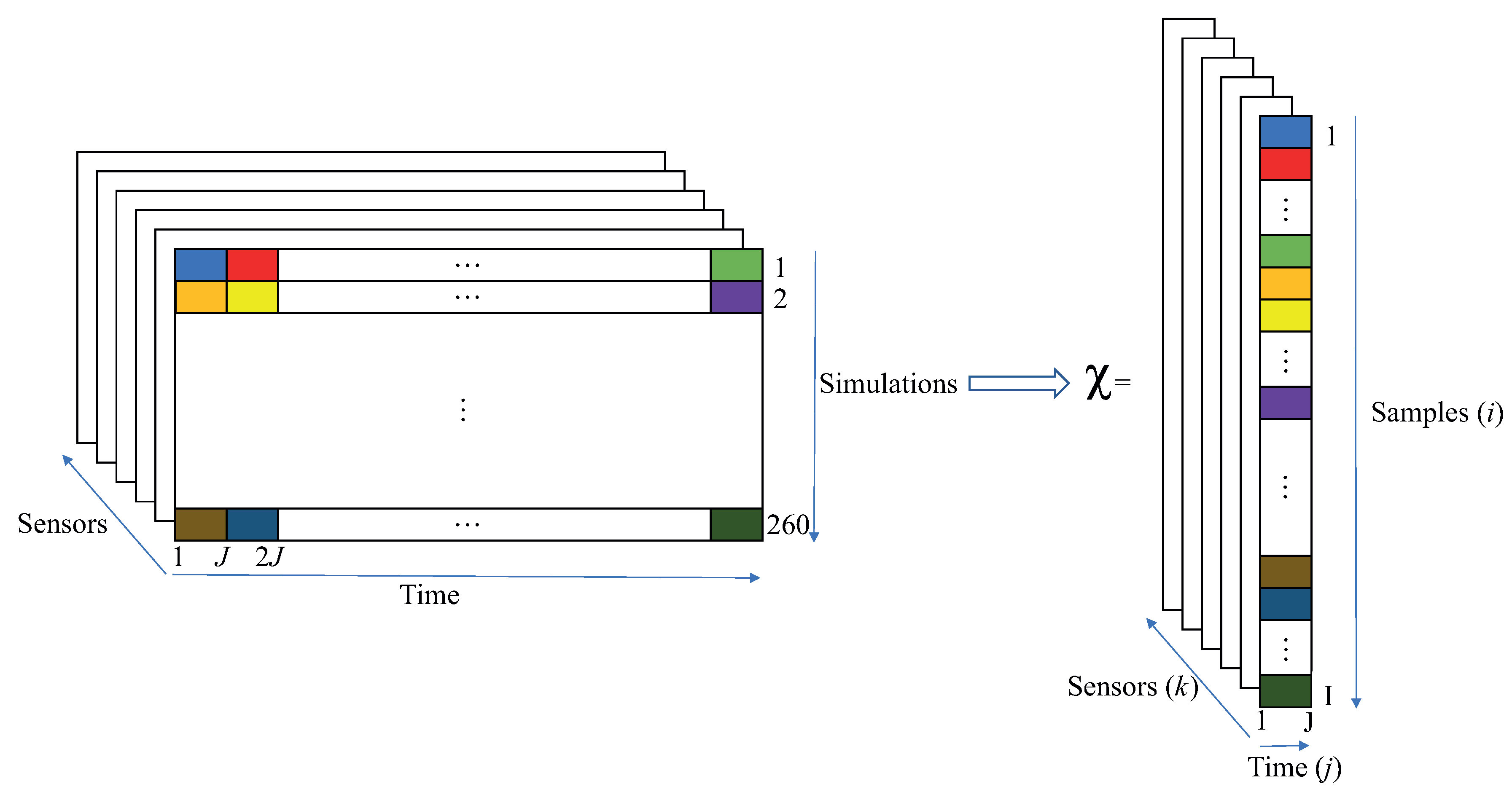
Figure 1 illustrates how the available data from the 260 long run simulations (see Equation (1)) were reorganized in a third-order tensor (multidimensional array with three indices) with short time samples of J time steps (see Equation (2)). The first J data-points determine the first sample (represented by the light blue color box in Figure 1). Immediately after, the next J data-points determine the second sample (red color box), etc. After the last J data-points of the first simulation (light green), the first J data-points of the second simulation (orange box) define the next sample, and so on. In general, let us consider that we have different sensors $k=1,2,\dots ,K$ stored at $j=1,2,\dots ,J$ time instants. Similar data are generated for a number of samples $i=1,2,\dots ,I$. This results in the third-order tensor $\mathcal{X}$ $(I\times J\times K)$ as illustrated in Figure 1, where the height (I) gives the number of samples; the width (J) gives the number of time instants; and the length (K) gives the number of sensors.

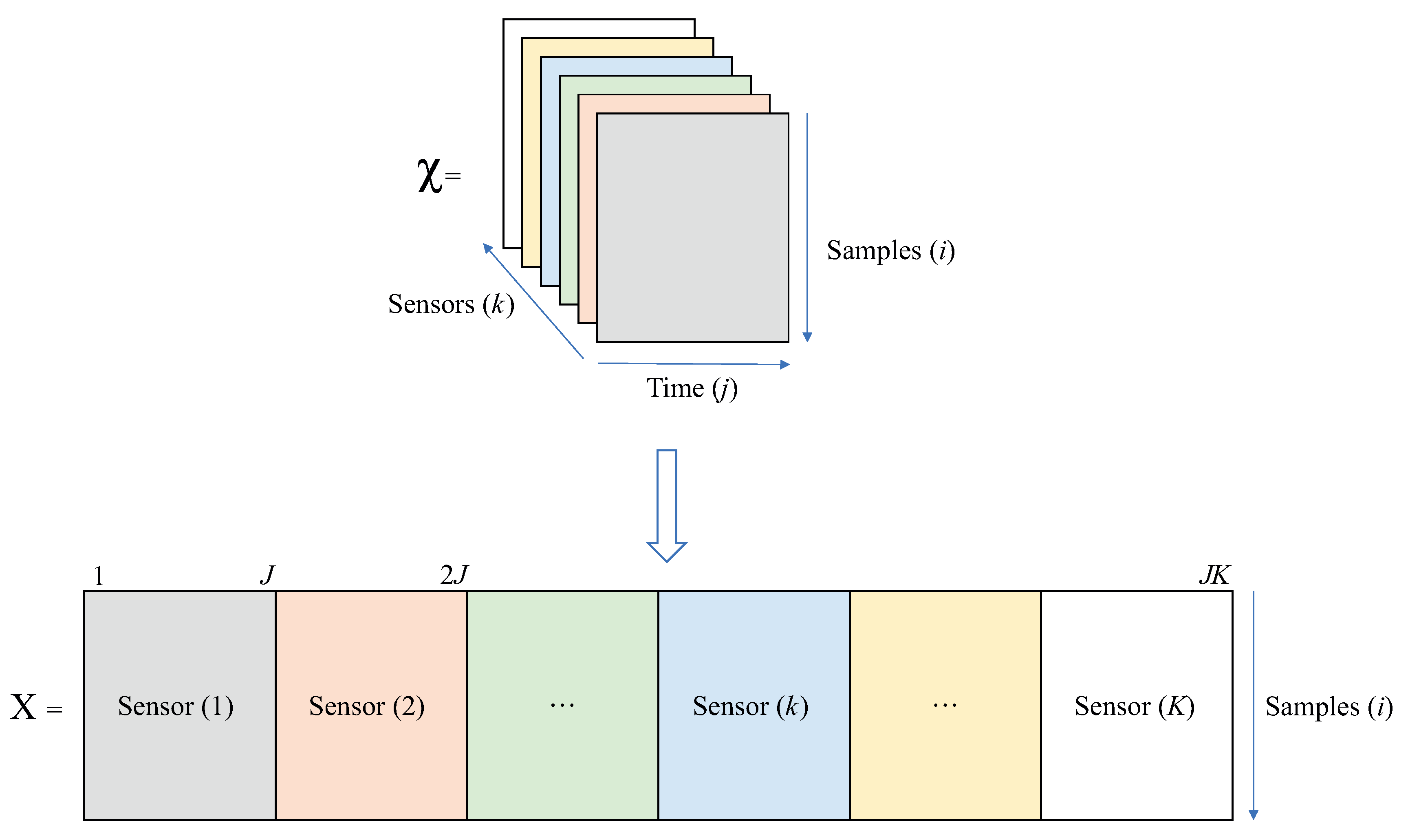
The crux of the matter for fault detection by SVM is the definition of the features to be used for classification [13]. In this work, statistical analysis by multiway PCA is used for pretreatment of the raw data. This is equivalent to implementing basic PCA on a large two-dimensional matrix assembled by unfolding the third-order tensor $\mathcal{X}$, see Figure 1. There are three possible ways of unfolding this tensor, as suggested by [28]. In general, sample-wise unfolding facilitates the analysis of the variability among samples by summarizing the information related to the measured variables (sensors) and their variations over time. Thus, in this work, the sample-wise unfolding is used (see Figure 2), where

$$\begin{array}{c}\hfill \mathcal{X}(I\times J\times K)⟶X(I\times JK).\end{array}$$

(3)

That is, the $I\times J$ planes are concatenated into a large two-dimensional matrix X. In summary, multiway PCA of the third-order tensor $\mathcal{X}$ in Figure 1 is implemented considering PCA of the sample-wise unfolded matrix X in Equation (2).

2.5. Autoscaling or Standardization

There are two reasons for autoscaling the raw data: to deal with data that come from different sensors and with different magnitudes, and to simplify the computations for the multiway PCA decomposition.

Autoscaling is a relatively common pre-processing method that uses column-wise mean-centering followed by division of each column by the standard deviation of that column of matrix X. The result is that each column of the new autoscaled matrix, $\tilde{X}$, has a mean of zero and a standard deviation of one. This idea is used in this work to rectify for different sensor measurements, magnitudes, and units where the prevalent source of variance is due to the signal itself rather than noise. In particular, it is computed as

$$\begin{array}{cc}\hfill {\mu }_j& =\frac{1}{I}\sum _{i=1}^I{x}_{ij},j=1,\dots ,JK,\hfill \end{array}$$

(4)

$$\begin{array}{cc}\hfill {\sigma }_j& =\sqrt{\frac{1}{I}\sum _{i=1}^I{(x_{ij}-{\mu }_j)}^2},j=1,\dots ,JK,\hfill \end{array}$$

(5)

where ${\mu }_j$ and ${\sigma }_j$ are the mean and the standard deviation, respectively, of all the measures at column j. Accordingly, the elements of matrix X are normalized to create a new matrix $\tilde{X}$ as

$$\begin{array}{cc}\hfill {\tilde{x}}_{ij}& :=\frac{x_{ij}-{\mu }_j}{{\sigma }_j},i=1,\dots ,I,j=1,\dots ,JK.\hfill \end{array}$$

(6)

2.6. Multiway PCA

Recall that before using a classifier, the raw data coming from the sensors must be processed to obtain the most suitable features. In this work, after the autoscaling step, multiway PCA was selected, as the main objective was to keep as much information as possible with the minimum amount of data.

Since the input data are given in a mean-centered matrix $\tilde{X}$, the empirical covariance matrix, S, can be computed as

$$\begin{array}{c}\hfill S=\frac{1}{I-1}{\tilde{X}}^T\tilde{X}\in {\mathcal{M}}_{\left(JK\right)\times \left(JK\right)}\left(\mathbb{R}\right).\end{array}$$

(7)

Then, the singular value decomposition of S is computed as

$$\begin{array}{c}\hfill S=PD{P}^T,\end{array}$$

(8)

where D is a matrix in diagonal form composed of the eigenvalues ${\lambda }_1,{\lambda }_2,\dots ,{\lambda }_{JK}$ in decreasing order, and $P\in {\mathcal{M}}_{\left(JK\right)\times \left(JK\right)}\left(\mathbb{R}\right)$ is an orthogonal matrix that contains the eigenvectors. Matrix P is usually called the loading matrix. As the main objective is to reduce the overall size of the data set, only a reduced number of $d<JK$ principal components are used. In this work, the number of principal components was selected based on keeping 99.98% of the variance. The proportion of the variance directed along (explained by) the first d components is given by:

$$\begin{array}{c}\hfill \frac{{\lambda }_1+\cdots +{\lambda }_d}{{\lambda }_1+\cdots +{\lambda }_{JK}}.\end{array}$$

(9)

In the first case, when $J=3$, from a total of $J\times K=3\times 9=27$ components, 99.98% of the variance is accomplished by the first $d=16$ components. When $J=8$, from a total of $J\times K=8\times 9=72$ components, the first $d=42$ components are needed to keep 99.98% of the variance. Finally, when $J=10$, from a total of $J\times K=10\times 9=90$ components, the demanded variance is accomplished by the first $d=52$ components. Thus, the matrix $P_d\in {\mathcal{M}}_{\left(JK\right)\times \left(d\right)}\left(\mathbb{R}\right)$, with only the first d columns of P is used. Finally, the score matrix $Y\in {\mathcal{M}}_{\left(I\right)\times \left(d\right)}\left(\mathbb{R}\right)$ (transformed coordinates of the $\tilde{X}$ data in the new basis given by the first d principal components), whose columns will be used as features by the SVM strategy, is computed as

$$\begin{array}{c}\hfill Y=\tilde{X}{P}_d.\end{array}$$

(10)

2.7. Support Vector Machines

Since their introduction by Vladimir Vapnik [29], SVMs have been successfully applied to a number of real-world problems such as face detection, object detection, and handwritten digit and character recognition in machine vision. SVMs exhibit a remarkable resistance to overfitting, and their training is performed by maximizing a convex functional, which means that there is a unique solution that can always be found in polynomial time [30]. In this section, basic information about SVM classification is given.

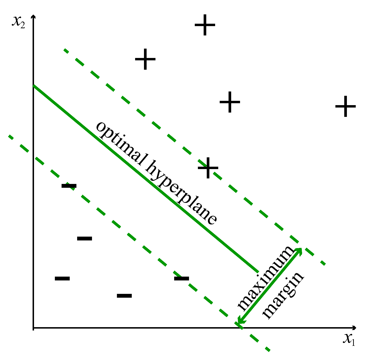
SVM classification is fundamentally a binary classification technique. Let us consider a training set ${\left\{(x_i,y_i)\right\}}_{i=1}^N$ with d-dimensional data $x_i\in {\mathbb{R}}^d$ and their corresponding label $y_i\in \{-1,+1\}$. Figure 3 shows these data where one class is labeled as (+) and the other one as (−). The main goal is to find the optimal hyperplane that defines the widest margin to separate both classes, see Figure 3. Formally, the hyperplane is given by

$$\begin{array}{c}\hfill h\left(x\right)={\omega }^{T}x+b,\end{array}$$

(11)

where b is known as the bias term and $\omega$ is the weight vector. The optimal hyperplane can be characterized in an infinite number of different ways by scaling of b and $\omega$. As a matter of agreement, among all the possible descriptions of the hyperplane, the so-called canonical hyperplane is chosen that satisfies

$$\begin{array}{cc}\hfill {\omega }^T{x}_{+}^{sv}+b& =1,\hfill \end{array}$$

(12)

$$\begin{array}{cc}\hfill {\omega }^T{x}_{-}^{sv}+b& =-1,\hfill \end{array}$$

(13)

where $x_{+}^{sv}$ and $x_{-}^{sv}$ symbolize the (+) and (−) training samples closest to the hyperplane, that is the so-called support vectors, see Figure 3. The distance between a point x and the hyperplane h is given by

$$\begin{array}{c}\hfill \mathrm{d}(x,h)=\frac{|{\omega }^{T}x+b|}{\left|\right|\omega \left|\right|}.\end{array}$$

(14)

In particular, for the canonical hyperplane, when x is a support vector, the numerator $|{\omega }^{T}x+b|$ is equal to one and the distance to the support vector is

$$\begin{array}{c}\hfill \mathrm{d}(x_{\pm }^{sv},h)=\frac{1}{\left|\right|\omega \left|\right|}.\end{array}$$

(15)

The width of the margin is twice this distance (i.e., $\frac{2}{\left|\right|\omega \left|\right|}$). Thus, maximizing the margin is equivalent to minimizing the expression $\frac{\left|\right|\omega \left|\right|}{2}$, which is equivalent to the following minimization problem:

$$\begin{array}{c}\hfill \underset{\omega ,b}{min}\frac{1}{2}{\left|\right|\omega \left|\right|}^2\mathrm{subject}\mathrm{to}\left\{\begin{array}{c}h\left(x_i\right)\ge 1,\forall y_i=1\mathrm{samples};\hfill \\ h\left(x_i\right)\le -1,\forall y_i=-1\mathrm{samples}.\hfill \end{array}\right.\end{array}$$

(16)

The two previous restrictions can be rewritten in one single equation by taking the product $h\left(x\right)y$,

$$\begin{array}{c}\hfill \underset{\omega ,b}{min}\frac{1}{2}{\left|\right|\omega \left|\right|}^2\mathrm{subject}\mathrm{to}h\left(x_i\right)y_i\ge 1,i=1,\dots ,N.\end{array}$$

(17)

This problem, to find the extrema of a function with constraints, can be solved using Lagrange multipliers, thus leading to

$$\underset{\omega ,b}{min}L(\omega ,b)=\frac{1}{2}{\left|\right|\omega \left|\right|}^2-\sum _{i=1}^N{\alpha }_i\left[y_i({\omega }^T{x}_i+b)-1\right],$$

(18)

where ${\alpha }_i$ are the Lagrange multipliers. Taking partial derivative with respect to $\omega$ equal to zero,

$$\frac{\partial L(\omega ,b)}{\partial \omega }=\omega -\sum _{i=1}^N{\alpha }_i{y}_i{x}_i=0\iff \omega =\sum _{i=1}^N{\alpha }_i{y}_i{x}_i.$$

(19)

This equation states that the decision vector, $\omega$, is a linear combination of the data samples. Taking partial derivative with respect to b equal to zero,

$$\frac{\partial L(\omega ,b)}{\partial b}=-\sum _{i=1}^N{\alpha }_i{y}_i=0.$$

(20)

Finally, substitution of Equations (19) and (20) into Equation (18) leads to

$$\underset{{\alpha }_i}{min}\left[\frac{1}{2}{\left(\sum _{i=1}^N{\alpha }_i{y}_i{x}_i\right)}^T\left(\sum _{j=1}^N{\alpha }_j{y}_j{x}_j\right)-\sum _{i=1}^N{\alpha }_i{y}_i{\left(\sum _{j=1}^N{\alpha }_j{y}_j{x}_j\right)}^T{x}_i-b\underset{=0}{\underbrace{\sum _{i=1}^N{\alpha }_i{y}_i}}+\sum _{i=1}^N{\alpha }_i\right],$$

(21)

which can be rewritten as

$$\underset{{\alpha }_i}{min}\left[\sum _{i=1}^N{\alpha }_i-\frac{1}{2}\sum _{i=1}^N\sum _{j=1}^N{\alpha }_i{\alpha }_j{y}_i{y}_j{x}_i^T{x}_j\right].$$

(22)

If the data do not admit a separating hyperplane, SVM can use a soft margin, meaning a hyperplane that separates many, although not all data points. Consequently, the previous problem is generalized by means of slack variables, ${\epsilon }_i$, and a penalty parameter, C. The general formulation for the linear kernel is in this case:

$$\begin{array}{c}\hfill \underset{\omega ,b,{\epsilon }_i}{min}\frac{1}{2}{\left|\right|\omega \left|\right|}^2+C\sum _{i=1}^N{\epsilon }_i\mathrm{subject}\mathrm{to}\left\{\begin{array}{c}h\left(x_i\right)y_i\ge 1-{\epsilon }_i,i=1,\dots ,N;\hfill \\ {\epsilon }_i\ge 0,i=1,\dots ,N.\hfill \end{array}\right.\end{array}$$

(23)

In this case, using Lagrange multipliers, the problem reads

$$\begin{array}{c}\hfill \underset{{\alpha }_i}{min}\left[\sum _{i=1}^N{\alpha }_i-\frac{1}{2}\sum _{i=1}^N\sum _{j=1}^N{\alpha }_i{\alpha }_j{y}_i{y}_j{x}_i^T{x}_j\right]\mathrm{subject}\mathrm{to}\left\{\begin{array}{c}{\sum }_{i=1}^N{\alpha }_i{y}_i=0;\hfill \\ 0\le {\alpha }_i\le C,i=1,\dots ,N.\hfill \end{array}\right.\end{array}$$

(24)

The final set of restrictions shows why the penalty parameter C is frequently called a box constraint, as it keeps the admissible values of the Lagrange multipliers in a bounded region. In this work, the box constraint value was tuned to optimize the performance of the SVM, as shown in Section 4.

From Equations (22) and (24), it is obvious that optimization depends only on dot products of pairs of samples. Additionally, the decision rule depends only on the dot product. Furthermore, the optimization problem is solved in a convex space (in contrast to neural networks), thus it never obtains a local extrema but the global one. When the space is not linearly separable (the classification problem does not have a simple hyperplane as a useful separating criterion even using a soft margin), a transformation to another space can be used, $\varphi (·)$. In fact, the transformation itself is not needed, but just the dot product, the so-called kernel function:

$$\begin{array}{c}\hfill K(x_i,x_j)=\varphi \left(x_i\right)\varphi \left(x_j\right).\end{array}$$

(25)

The kernel function permits the computation of the inner product between the mapped vectors without expressly calculating the mapping. This is advantageous, as it implies that if data are transformed into a higher-dimensional space (which helps to better classification) there is no need to compute the exact transformation of the data, but only the inner product of the data in that higher-dimensional space (which is computationally cheaper). This is known as the “kernel trick” [31]. Different kernels can be used, namely polynomial, hyperbolic tangent, or Gaussian radial basis function. On one hand, the feature space mapping of the Gaussian kernel has infinite dimensionality. On the other hand, the Gaussian kernel has a ready interpretation as a similarity measure, as its value decreases with distance and ranges between zero and one. For these reasons, in this work the Gaussian kernel is used, namely,

$$\begin{array}{c}\hfill K(x_i,x_j)=e^{{\displaystyle -\gamma \left(\right||x_i-x_j|{|}^2)}},\end{array}$$

(26)

where $\gamma$ is a free parameter, hereafter denoted as kernel scale, related to the Gaussian kernel width. In this work, the kernel scale is computed as the inverse of the square root of the number of features. Note that in this work, the same features and the same kernel scale value for the Gaussian kernel are used to detect all faults. In other words, a unique trained SVM is able to classify among all the studied classes (i.e., eight faulty classes and one healthy class). That is not the case in the previous literature related to WT fault detection (e.g., [13,32]) where the features and the variance were adjusted case-by-case to detect each different fault, thus leading to a much more complex strategy that needed as many different SVM classifiers as faults to detect. Regarding computational effort, there is a clear advantage related to the feature computation, as only one set of features is needed in our proposed approach.

As was mentioned earlier, SVM classification is essentially a binary (i.e., two-class) classification technique, which has to be modified to deal with the multi-fault classification. Two of the most common methods to enable this adaptation include the one-vs.-one and one-vs.-all approaches. The one-vs.-all technique represents the earliest and most common SVM multiclass approach [33], and comprises the division of an N class dataset into N two-class cases, and it chooses the class which classifies the test with greatest margin. The one-vs.-one strategy comprises constructing a machine for each pair of classes, thus resulting in $N(N-1)/2$ machines. When this approach is applied to a test point, each classification gives one vote to the winning class, and the point is labeled with the class having the most votes. The one-vs.-one strategy is more computationally demanding because the results of more SVM pairs need to be computed. In this work, the one-vs.-all approach is used.

2.8. k-Fold Cross-Validation

Normally, a data-based classifier is inferred based on training data and considering a classifier learning algorithm. A prediction error—also known as true error—is associated to each classifier. However, this prediction error is usually unknown, cannot be computed, and must be estimated based on data. Different estimators of the prediction error can be considered, from the simple hold-out [34] and resubstitution [35] to the more sophisticated bootstrap [36]. One of these techniques, and possibly the most popular, is k-fold cross-validation [37]. In k-fold cross-validation, the data set is distributed into k folds, the classifier is then learned using $k-1$ folds, and the prediction error is computed by testing the classifier in the fold that is not used in the learning step. In the end, the estimation of the error is the numerical mean of the errors committed in each fold. In this paper, 10-fold cross-validation is used to estimate the performance of the proposed FD strategy.

3. Results, Analysis, and Discussion

The results of the proposed multi-fault diagnosis strategy introduced in Section 2 in the dataset under study are presented in this section.

It is worth mentioning that, as can be seen in Section 1, there is an increasing number of studies in the field of structural health monitoring or condition monitoring based on machine learning approaches. In this work, the contribution resides essentially in how data are collected, how data are arranged, how data are pre-processed, and how SVM is applied. For instance, in [38,39] it can be noted that there are six possible ways of arranging a third-order tensor. Each one of these six possible choices will lead to a different overall performance of the applied strategy. A similar thing can be said with respect to SVM. As was pointed out in Section 2.7, SVM depends on several parameters and kernels. In this work, the same features and the same variance for the Gaussian kernel are used to detect all the faults, therefore leading to a single trained classifier.

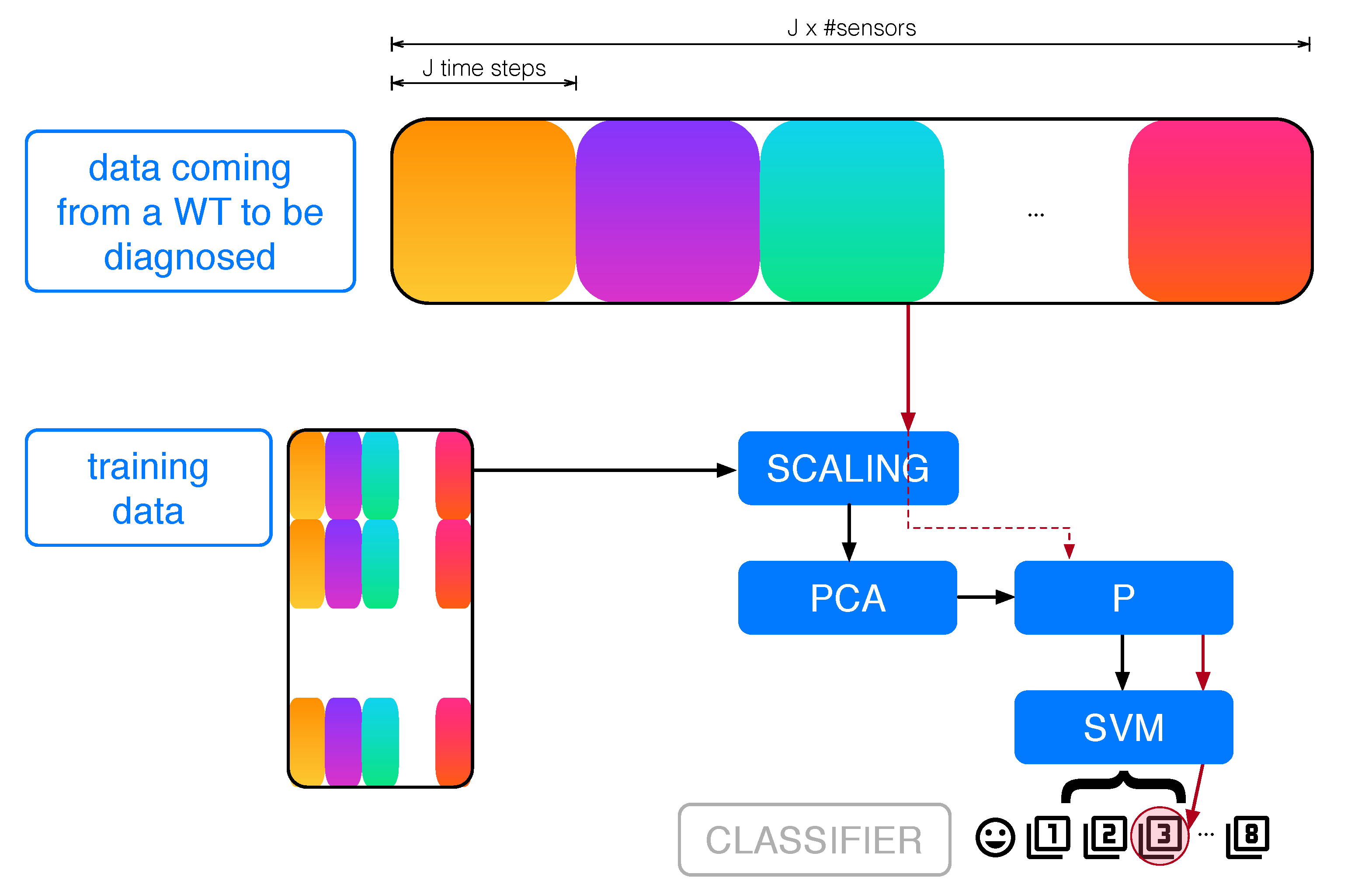
First, a flowchart of the proposed approach and how it is applied is given in Figure 4. When a WT has to be diagnosed, data coming from the WT sensors are scaled and then, using the already-computed PCA projection, the features are computed. Then, the already-trained SVM classifies the data.

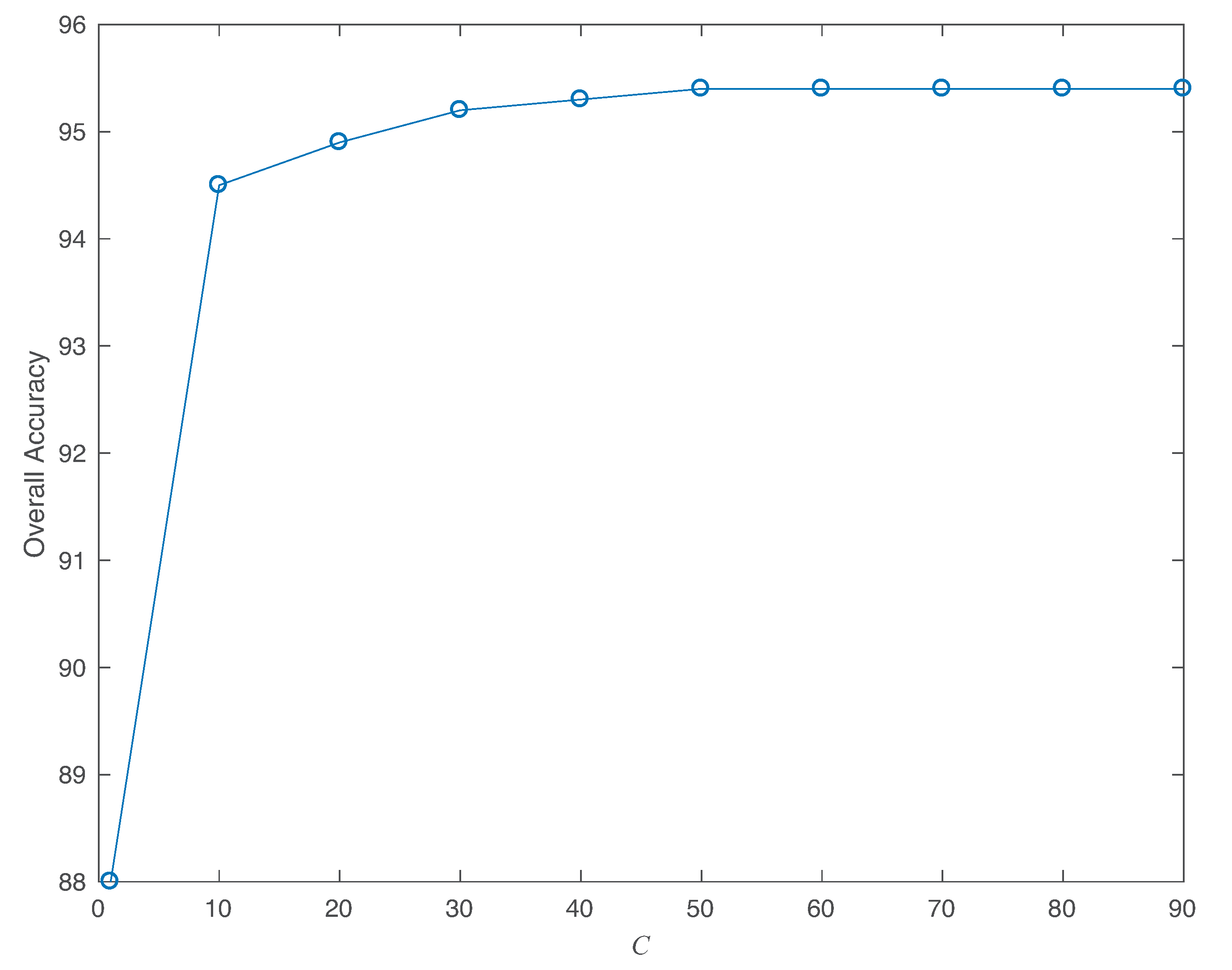
The box constraint value is tuned to optimize the SVM performance. Making this value large increases the weight of misclassification, see Equation (23), which leads to a stricter separation. However, increasing its value leads to longer training times. The value $C=50$ was used in this work because, as shown in Figure 5, with smaller values the overall accuracy was degraded and with larger values similar results were obtained (with longer training times).

Table 4. Summary of the obtained results.

Performance	$\mathit{J}=3$	$\mathit{J}=8$	$\mathit{J}=10$
Accuracy (%)	95.5	98	98.2
Training time (s)	2990	202	181
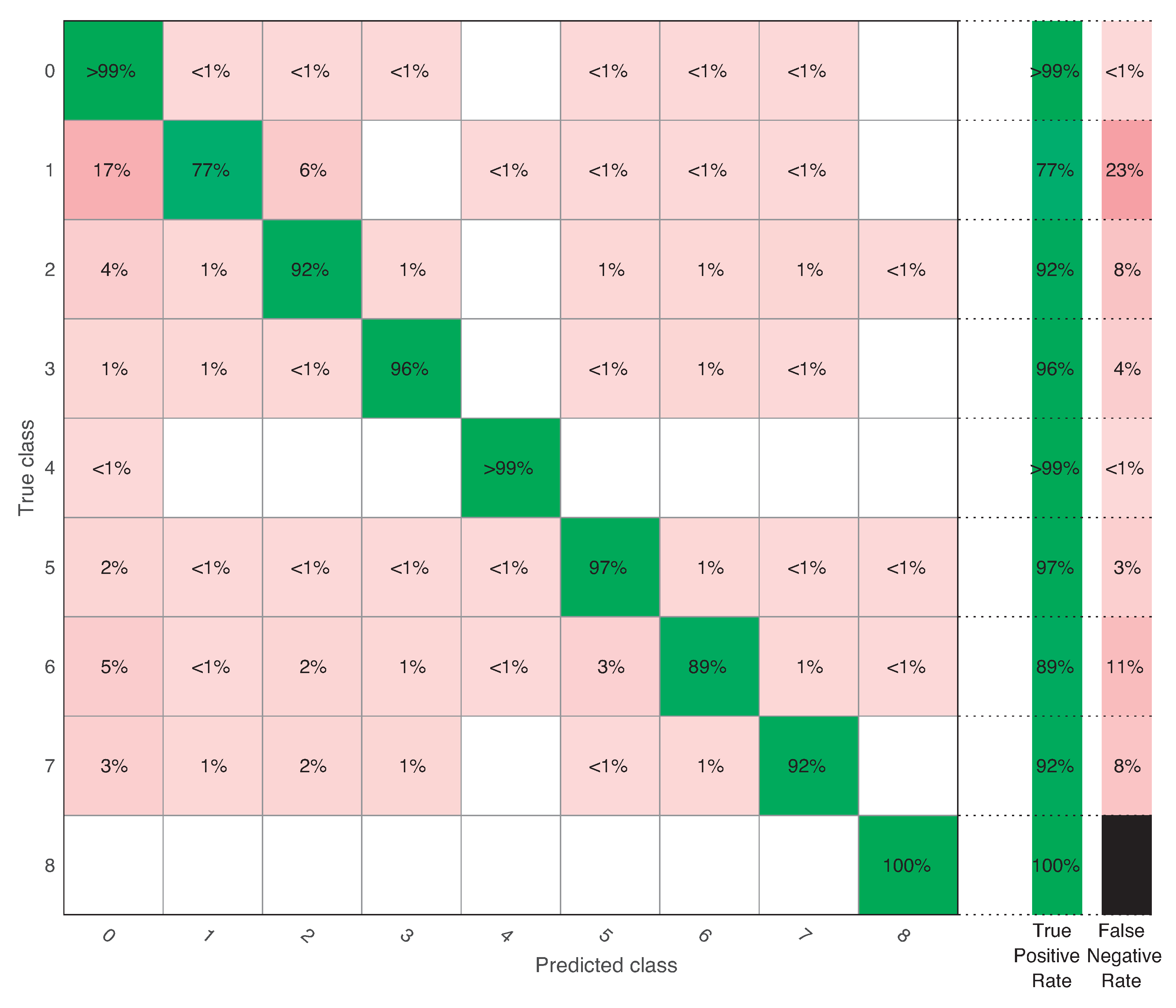
Prediction speed (obs/s)	3000	3500	3600

summarizes the results obtained from the proposed strategy. It presents not only the overall accuracy, but also the training time and prediction speed, as both parameters are critical in real application. Notice that in all cases, the prediction speed allows this strategy to be deployed for online (real-time) condition monitoring in WTs. Besides, a comprehensive decomposition of the error between the true classes and the predicted classes is shown by means of the so-called confusion matrices, see Figure 6, Figure 7 and Figure 8 (an empty blank square means 0%). In these matrices, each row represents the instances in a true class while each column represents the instances in a predicted class (by the classifier). In particular, the first row (and first column) is labeled as 0 and corresponds to the healthy case. The next labels (for rows and columns) correspond to each fault (from Fault 1 to Fault 8). From the confusion matrices and Table 4, the following issues can be highlighted.

When detection time was approximately 3 s ($J=3$), the overall accuracy was $95.5$%. In this case, the healthy class had a true positive rate (TPR, the percentage of correctly classified instances) higher than 99% and a false negative rate (FNR, the percentage of incorrectly classified instances) smaller than 1%. Fault 1 (the most difficult to classify in previous references and related to the pitch actuator fault with high dynamics) had a TPR of 77% and an FNR of 23%. This FNR percentage was mainly obtained from 17% missing faults and 6% confusion with Fault 2, which is also a fault located in the pitch actuator. Fault 6, related to a stuck value (10 deg) of the pitch sensor measurement, was misclassified as healthy 5% of the time, 3% of the time it was confused with the same type of fault but with only a 5 deg stuck value (Fault 5), and 2% of the time it was misclassified as Fault 2 (pitch actuator fault). The other faults had a TPR higher than 92%. Note that Fault 8, the most severe one and related to the torque actuator, had a 100% TPR with this most restrictive detection time.

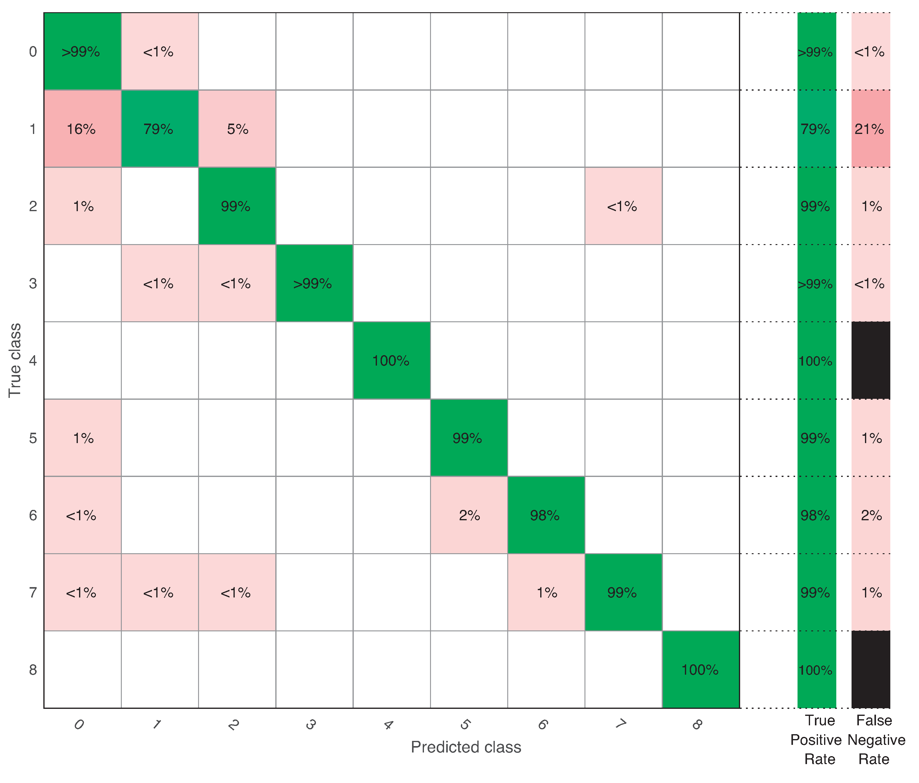
When detection time was approximately 8 s ($J=8$), the overall accuracy was 98%. As in the previous case, the healthy class had a TPR higher than 99%. Fault 1 increased its TPR to 79% (where 16% were missed faults and 5% confusion with Fault 2), and all the other classes increased their TPR to values higher than 98%. Note that Fault 4, related to the generator speed sensor, reached a 100% TPR. The generator speed measurement from the sensor was used as input in the torque and pitch controllers, and thus being able to correctly diagnose this type of fault is extremely important. As in the previous case, Fault 8 kept a 100% TPR.

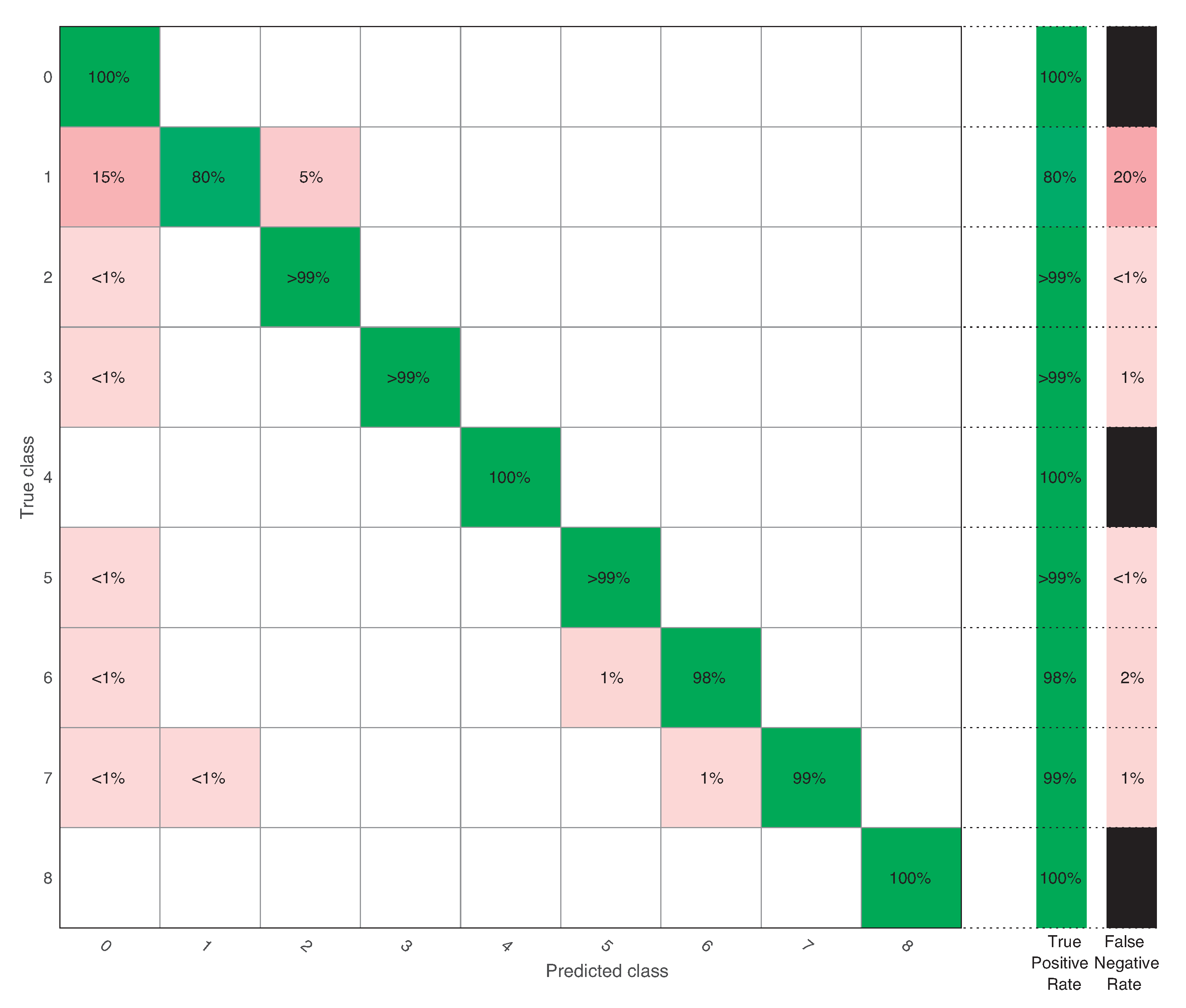
Finally, when $J=10$ the overall accuracy was 98.2%. In this case, Fault 1 was improved to have a TPR of 80%. In this case, all misclassifications were 1% or lower, except for Fault 1 that was misclassified as healthy 15% of the time and misclassified as Fault 2 5% of the time (recall that this is also a pitch actuator fault). Observe that Faults 1, 4, and 8 obtained a remarkable 100% TPR.

Access to real SCADA datasets is often proprietary, and therefore they are not accessible by the scientific community. To overcome this difficulty, in this work simulated data were obtained by one of the most widely accepted WT simulators in the scientific community (FAST). The drawbacks of using simulated data is that there is no possibility to evaluate the proposed method in a full test set representing the true distribution of real-world data where class imbalance is a challenging problem [40]. However, there are several references (e.g., [11]) where this problem is solved in the training stage using under/oversampling of the training data.

4. Conclusions

Because of its standard low sampling rate, there is a lack of knowledge on the potential of SCADA data for condition monitoring. In this work, a promising strategy to detect and classify multiple WT faults was presented using only conventional SCADA data with an additional, but feasible, high-frequency sampling from the sensors (1 sample/s). That is, the FD strategy does not involve the supplementary installation of costly purpose-built data sensing equipment for wind power plants.

Note that in this work, in contrast to the previous literature, the same features and the same variance for the Gaussian kernel were used to detect all the faults detailed in the benchmark. Thus, leading to a unique trained classifier capable of coping with all the studied faults by computing only one set of features from the data to diagnose. Consequently, the strategy that we propose outperformed other approaches.

As future work, other faults will be included involving misalignment, ice accumulation, and tower damage. Finally, we will study the contribution of an effective predictive maintenance strategy based on this same principle in order to further optimize operation and maintenance in WTs.

References

- Hossain, M.L.; Abu-Siada, A.; Muyeen, S.M. Methods for AdvancedWind Turbine Condition Monitoring and Early Diagnosis: A Literature Review. Energies 2018, 11, 1309. [Google Scholar] [CrossRef]
- Ahadi, A. Wind turbine fault diagnosis techniques and related algorithms. Int. J. Renew. Energy Res. (IJRER) 2016, 6, 80–89. [Google Scholar]
- De Azevedo, H.D.M.; Araújo, A.M.; Bouchonneau, N. A review of wind turbine bearing condition monitoring: State of the art and challenges. Renew. Sustain. Energy Rev. 2016, 56, 368–379. [Google Scholar] [CrossRef]
- Kandukuri, S.T.; Klausen, A.; Karimi, H.R.; Robbersmyr, K.G. A review of diagnostics and prognostics of low-speed machinery towards wind turbine farm-level health management. Renew. Sustain. Energy Rev. 2016, 53, 697–708. [Google Scholar] [CrossRef]
- Huang, S.; Wu, X.; Liu, X.; Gao, J.; He, Y. Overview of condition monitoring and operation control of electric power conversion systems in direct-drive wind turbines under faults. Front. Mech. Eng. 2017, 12, 281–302. [Google Scholar] [Green Version]
- Yang, Z.; Chai, Y. A survey of fault diagnosis for onshore grid-connected converter in wind energy conversion systems. Renew. Sustain. Energy Rev. 2016, 66, 345–359. [Google Scholar] [CrossRef]
- Ochieng, F.X.; Hancock, C.M.; Roberts, G.W.; Le Kernec, J. A review of ground-based radar as a noncontact sensor for structural health monitoring of in-field wind turbines blades. Wind Energy 2018. [Google Scholar] [CrossRef]
- Shohag, M.A.S.; Hammel, E.C.; Olawale, D.O.; Okoli, O.I. Damage mitigation techniques in wind turbine blades: A review. Wind Eng. 2017, 41, 185–210. [Google Scholar] [CrossRef]
- Zhao, Y.; Li, D.; Dong, A.; Kang, D.; Lv, Q.; Shang, L. Fault Prediction and Diagnosis of Wind Turbine Generators Using SCADA Data. Energies 2017, 10, 1210. [Google Scholar] [CrossRef]
- Astolfi, D.; Castellani, F.; Scappaticci, L.; Terzi, L. Diagnosis of wind turbine misalignment through SCADA data. Diagnostyka 2017, 18, 17–24. [Google Scholar]
- Leahy, K.; Hu, R.L.; Konstantakopoulos, I.C.; Spanos, C.J.; Agogino, A.M.; O’Sullivan, D.T.J. Diagnosing and predicting wind turbine faults from SCADA data using support vector machines. Int. J. Progn. Health Manag. 2018, 9, 1–11. [Google Scholar]
- Mazidi, P.; Du, M.; Tjernberg, L.B.; Bobi, M.A.S. A performance and maintenance evaluation framework for wind turbines. In Proceedings of the 2016 International Conference on Probabilistic Methods Applied to Power Systems (PMAPS), Beijing, China, 16–20 October 2016; pp. 1–8. [Google Scholar] [CrossRef]
- Laouti, N.; Sheibat, N.; Othman, S. Support vector machines for fault detection in wind turbines. In Proceedings of the IFAC World Congress, Milano, Italy, 28 August–2 September 2011; Volume 2, pp. 7067–7707. [Google Scholar]
- Laouti, N.; Othman, S.; Alamir, M.; Sheibat-Othman, N. Combination of model-based observer and support vector machines for fault detection of wind turbines. Int. J. Autom. Comput. 2014, 11, 274–287. [Google Scholar] [CrossRef]
- Xiao, Y.; Hong, Y.; Chen, X.; Chen, W. The application of dual-tree complex wavelet transform (DTCWT) energy entropy in misalignment fault diagnosis of doubly-fed wind turbine (DFWT). Entropy 2017, 19, 587. [Google Scholar] [CrossRef]
- Abdelkrim, S.; Djamel, M.M.; Samia, A.; Hayet, M.; Mawloud, T. The MAED and SVM for fault diagnosis of wind turbine system. Int. J. Renew. Energy Res. (IJRER) 2017, 7, 758–769. [Google Scholar]
- Wang, K.S.; Sharma, V.S.; Zhang, Z.Y. SCADA data based condition monitoring of wind turbines. Adv. Manuf. 2014, 2, 61–69. [Google Scholar] [CrossRef] [Green Version]
- Gonzalez, E.; Stephen, B.; Infield, D.; Melero, J. On the use of high-frequency SCADA data for improved wind turbine performance monitoring. J. Phys. Conf. Ser. 2017, 926, 012009. [Google Scholar] [CrossRef] [Green Version]
- Odgaard, P.F.; Stoustrup, J.; Kinnaert, M. Fault tolerant control of wind turbines—A benchmark model. IFAC Proc. Vol. 2009, 42, 155–160. [Google Scholar] [CrossRef]
- KK Wind Solutions. Available online: http://www.kkwindsolutions.com/ (accessed on 10 September 2018).
- The MathWorks, Inc. Available online: http://www.mathworks.com/ (accessed on 10 September 2018).
- Odgaard, P.F.; Stoustrup, J.; Kinnaert, M. Fault-tolerant control of wind turbines: A benchmark model. IEEE Trans. Control Syst. Technol. 2013, 21, 1168–1182. [Google Scholar] [CrossRef]
- Odgaard, P.; Johnson, K. Wind Turbine Fault Diagnosis and Fault Tolerant Control—An Enhanced Benchmark Challenge. In Proceedings of the American Control Conference, Washington, DC, USA, 17–19 June 2013; pp. 1–6. [Google Scholar]
- Ruiz, M.; Mujica, L.E.; Alférez, S.; Acho, L.; Tutivén, C.; Vidal, Y.; Rodellar, J.; Pozo, F. Wind turbine fault detection and classification by means of image texture analysis. Mech. Syst. Signal Process. 2018, 107, 149–167. [Google Scholar] [CrossRef] [Green Version]
- Lackner, M.A.; Rotea, M.A. Passive structural control of offshore wind turbines. Wind Energy 2011, 14, 373–388. [Google Scholar] [CrossRef]
- Jonkman, J.; Butterfield, S.; Musial, W.; Scott, G. Definition of a 5-MW Reference Wind Turbine for Offshore System Development; Technical Report No. NREL/TP-500-38060; National Renewable Energy Laboratory: Golden, CO, USA, 2009. [Google Scholar]
- May, A.; McMillan, D.; Thöns, S. Economic analysis of condition monitoring systems for offshore wind turbine sub-systems. IET Renew. Power Gener. 2015, 9, 900–907. [Google Scholar] [CrossRef] [Green Version]
- Hong, X.; Xu, Y.; Zhao, G. LBP-TOP: A Tensor Unfolding Revisit. In Proceedings of the Asian Conference on Computer Vision, Taipei, Taiwan, 20–24 November; pp. 513–527.
- Vapnik, V. The Nature of Statistical Learning Theory; Springer: Berlin, Germany, 1995. [Google Scholar]
- Yang, C.H.; Chin, L.C.; Hsieh, S.C. Morse code recognition using support vector machines. In Proceedings of the IEEE EMBS Asian-Pacific Conference on Biomedical Engineering, Kyoto, Japan, 20–22 October 2003; pp. 220–222. [Google Scholar]
- Theodoridis, S.; Koutroumbas, K. Pattern Recognition; Elsevier: Amsterdam, The Netherlands, 2009. [Google Scholar]
- Santos, P.; Villa, L.F.; Reñones, A.; Bustillo, A.; Maudes, J. An SVM-based solution for fault detection in wind turbines. Sensors 2015, 15, 5627–5648. [Google Scholar] [CrossRef] [PubMed] [Green Version]
- Melgani, F.; Bruzzone, L. Classification of hyperspectral remote sensing images with support vector machines. IEEE Trans. Geosci. Remote Sens. 2004, 42, 1778–1790. [Google Scholar] [CrossRef] [Green Version]
- McLachlan, G. Discriminant Analysis and Statistical Pattern Recognition; John Wiley & Sons: Hoboken, NJ, USA, 2004; Volume 544. [Google Scholar]
- Devroye, L.; Wagner, T. Distribution-free performance bounds with the resubstitution error estimate (Corresp.). IEEE Trans. Inf. Theory 1979, 25, 208–210. [Google Scholar] [CrossRef]
- Efron, B.; Tibshirani, R.J. An Introduction to the Bootstrap; CRC Press: Boca Raton, FL, USA, 1994. [Google Scholar]
- Stone, M. Cross-validatory choice and assessment of statistical predictions. J. R. Stat. Soc. Ser. B Methodol. 1974, 36, 111–147. [Google Scholar]
- Westerhuis, J.A.; Kourti, T.; MacGregor, J.F. Comparing alternative approaches for multivariate statistical analysis of batch process data. J. Chemom. 1999, 13, 397–413. [Google Scholar] [CrossRef]
- Pozo, F.; Vidal, Y.; Salgado, Ó. Wind Turbine Condition Monitoring Strategy through Multiway PCA and Multivariate Inference. Energies 2018, 11, 749. [Google Scholar] [CrossRef]
- Leahy, K.; Gallagher, C.; O’Donovan, P.; Bruton, K.; O’Sullivan, D. A Robust Prescriptive Framework and Performance Metric for Diagnosing and Predicting Wind Turbine Faults Based on SCADA and Alarms Data with Case Study. Energies 2008, 11, 1738. [Google Scholar] [CrossRef]
Figure 1.
Reshape data from long-run simulations (left) into a third-order tensor with short time samples of J seconds (right).
Figure 2.
Unfolding of the third-order tensor into matrix X.
Figure 3.
Linear support vector machine (SVM) in a two-dimensional example.
Figure 4.
Data coming from a wind turbine (WT) to be diagnosed are first scaled, then projected into the vectorial space spanned by the first principal components, and finally the projection enters the classifier.
Figure 5.
Box constraint value with respect to overall accuracy.
Figure 6.
Confusion matrix when .
Figure 7.
Figure 8.