A New Analysis Model for Potential Contamination of a Shallow Aquifer from a Hydraulically-Fractured Shale


Abstract
:1. Introduction
2. Mathematical Model
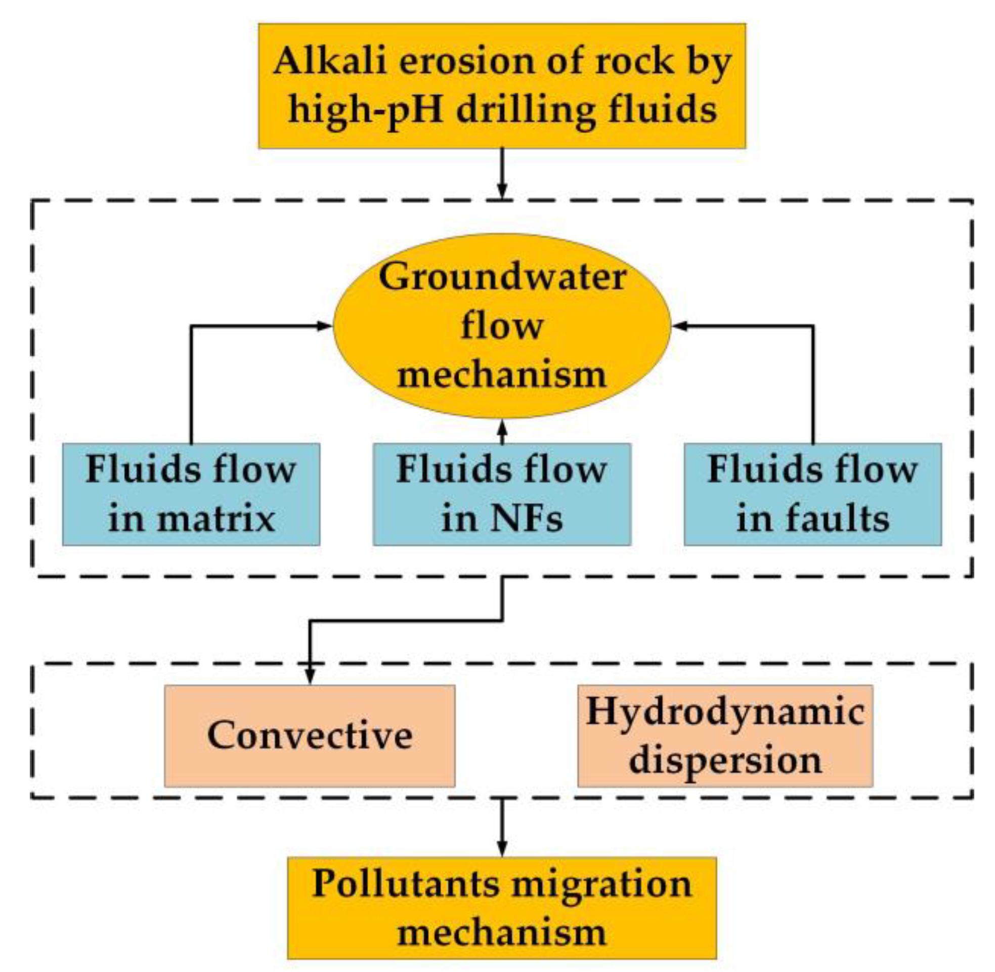
2.1. Groundwater Flow Mechanism
2.2. Contaminant Migration Mechanism
2.3. Alkali Erosion Mechanism of Rock by a High-pH Drilling Fluid
3. Model Verification
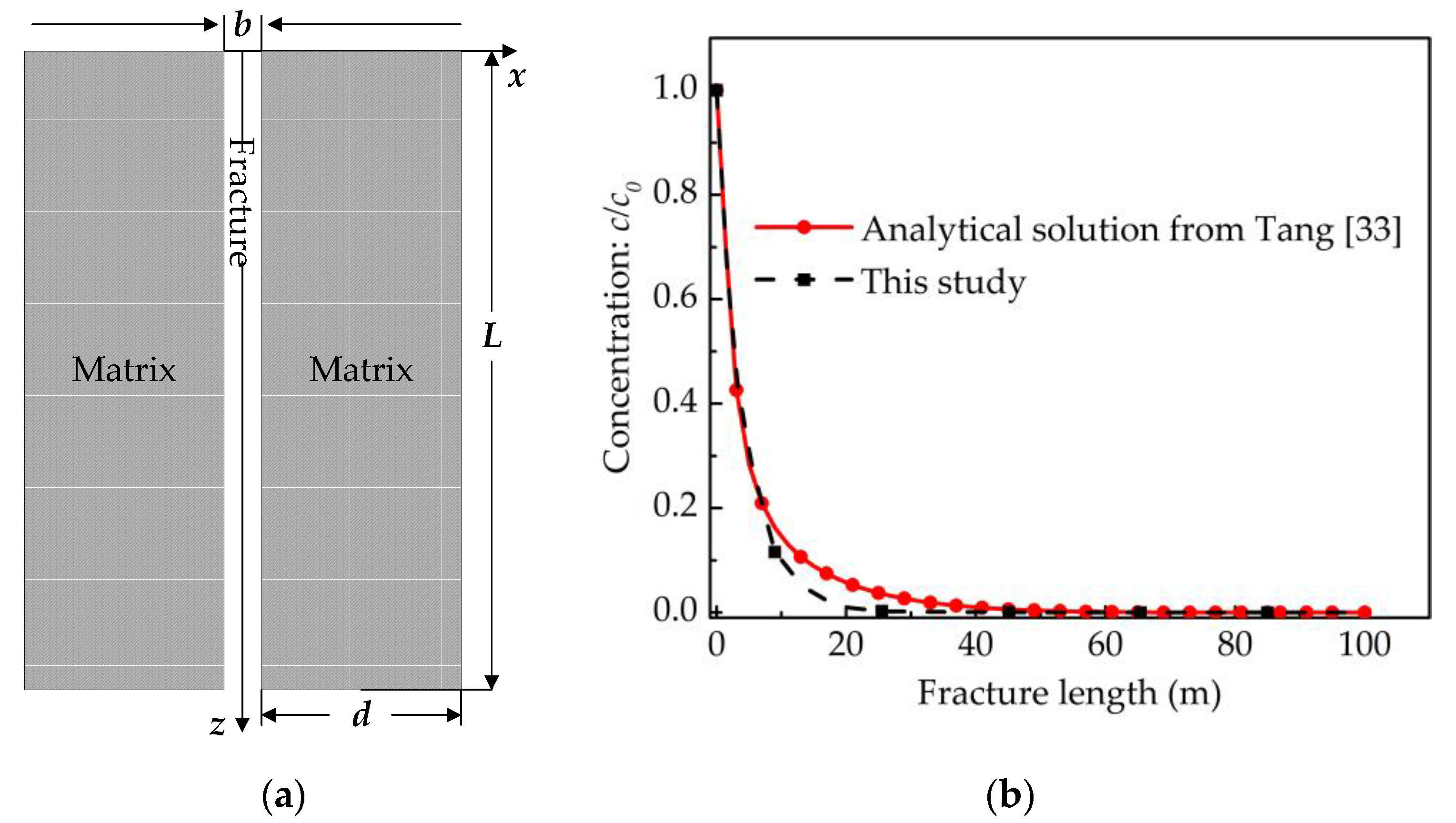
3.1. Case 1: Consideration of a Single Fracture
3.2. Case 2: Consideration of the Geological Distributions
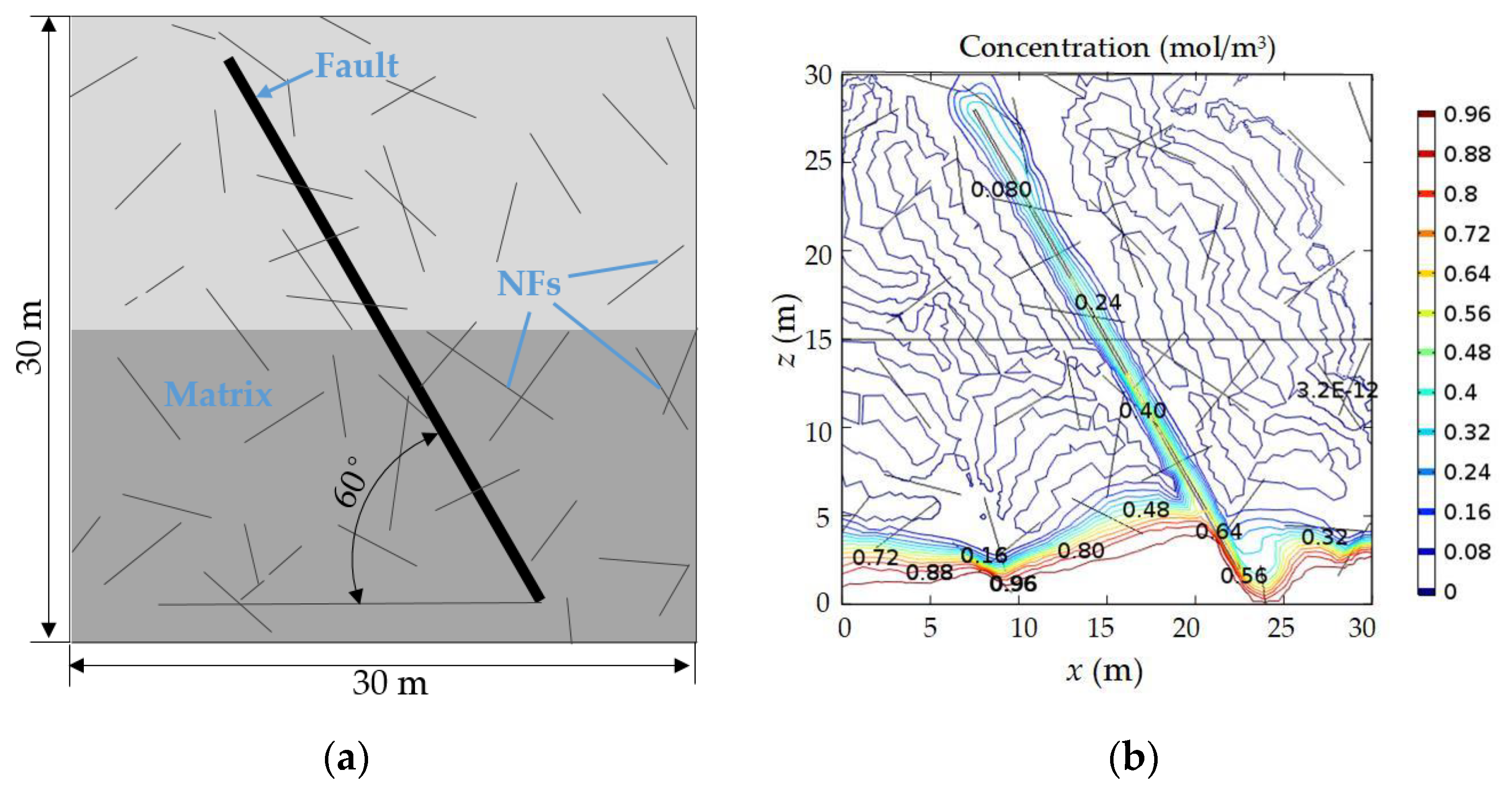
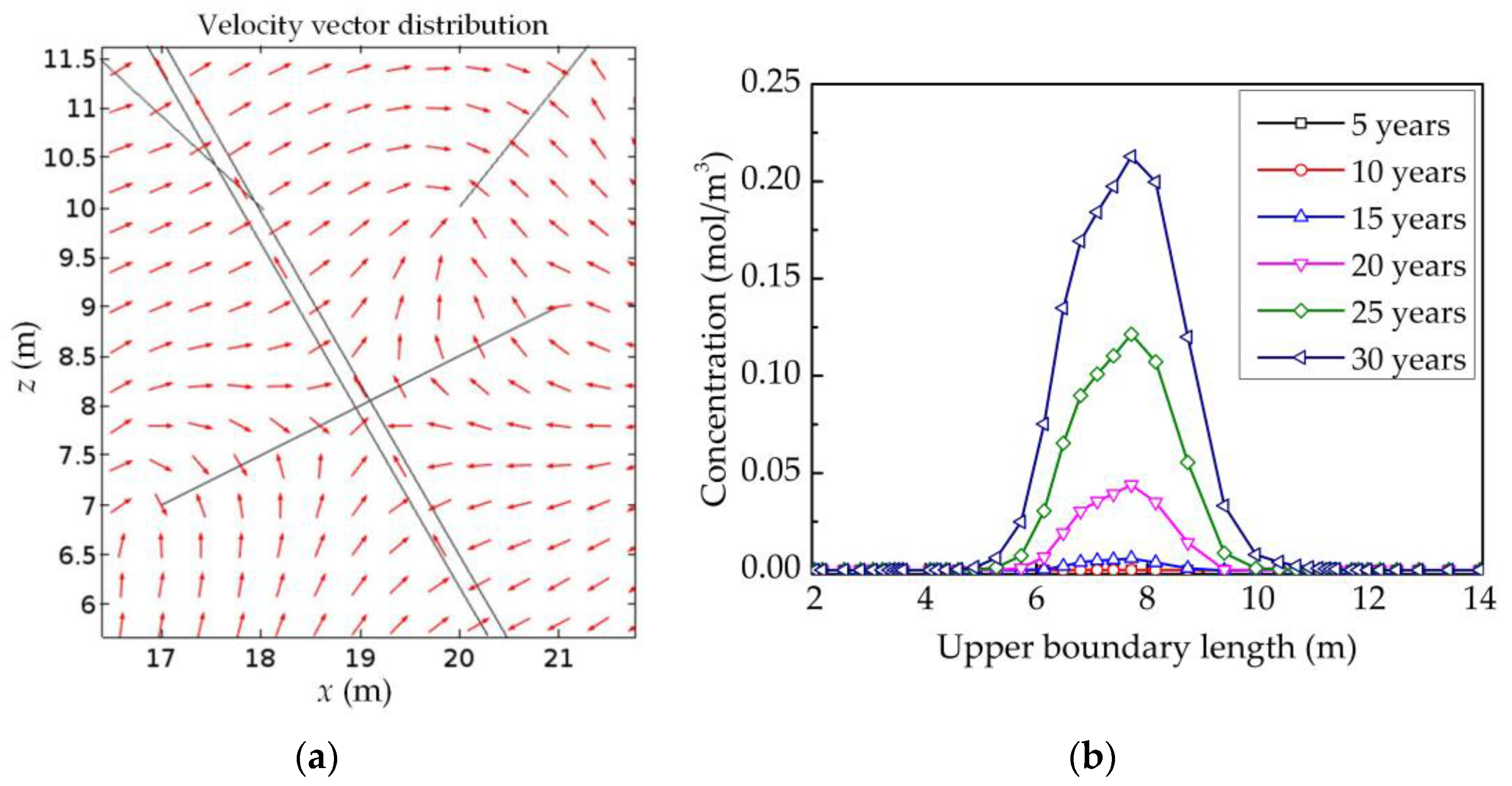
3.3. Case 3: Consideration of the NFs
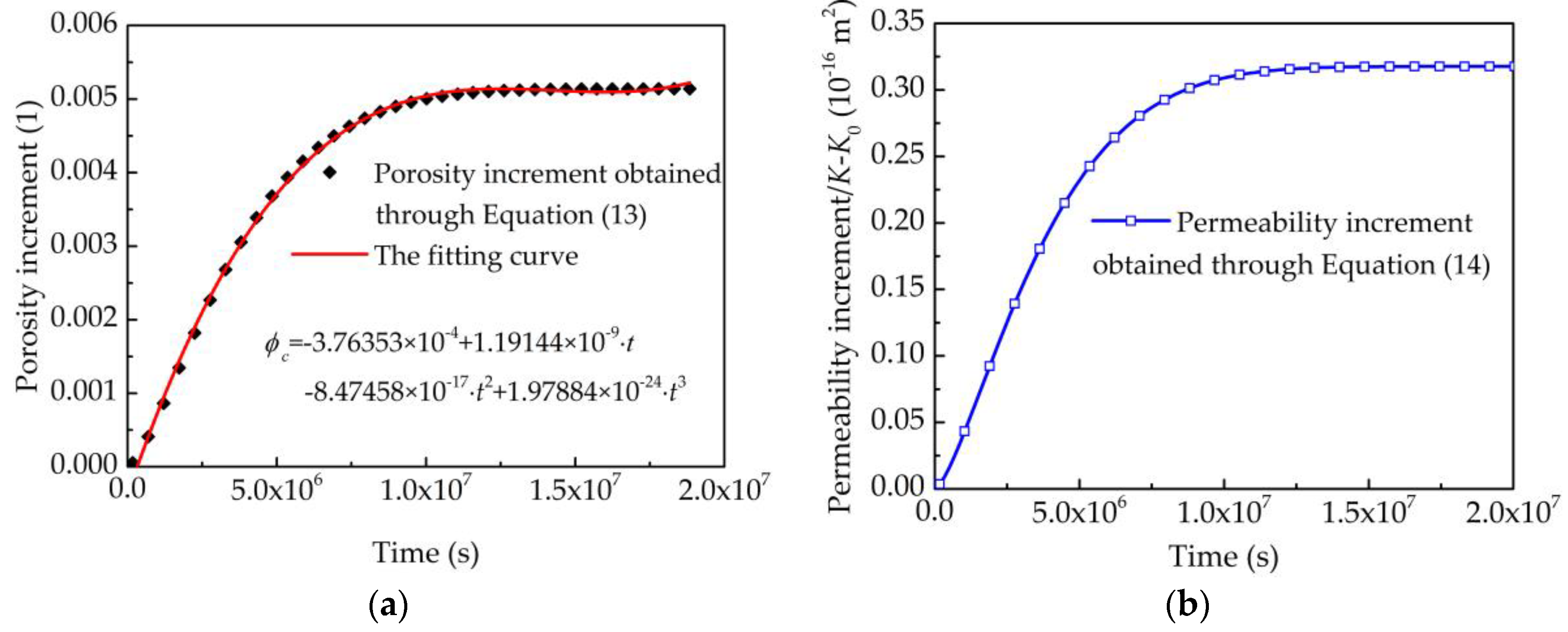
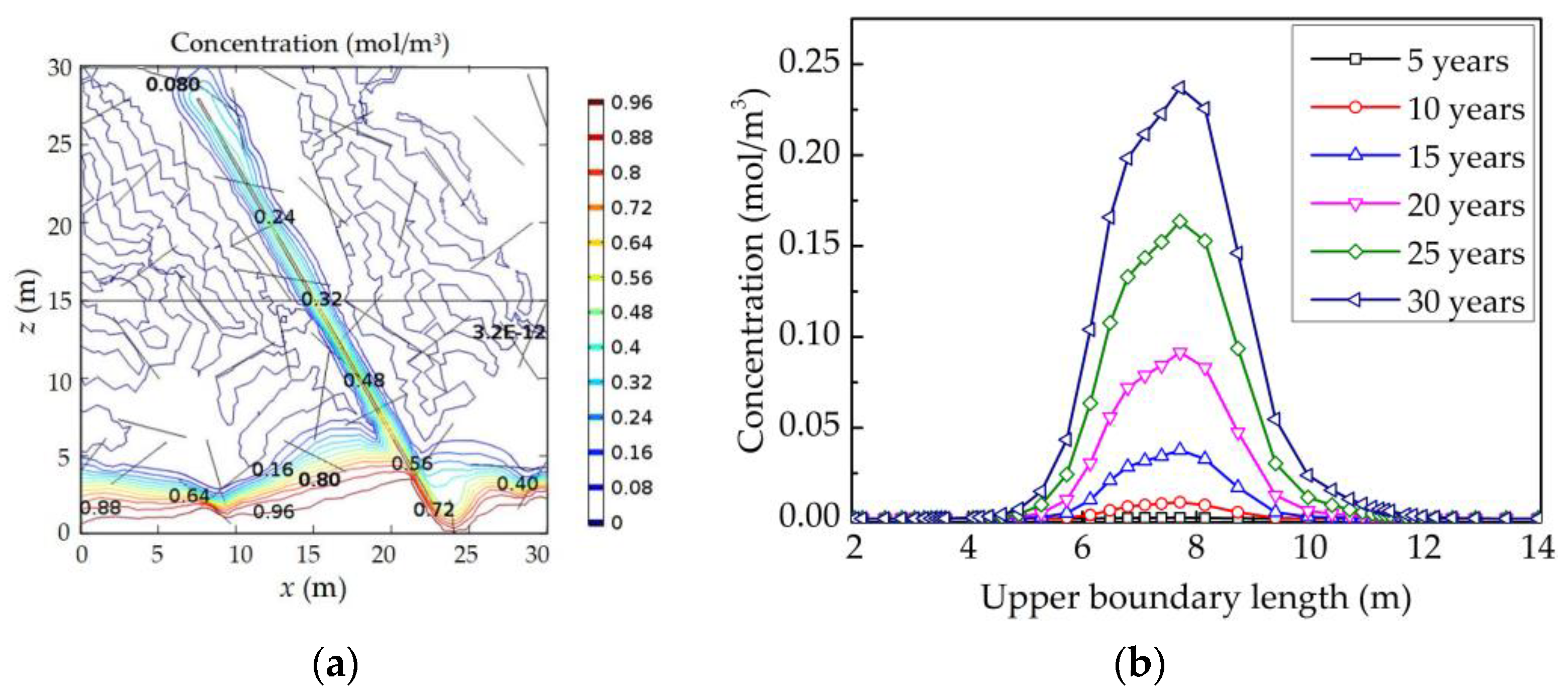
3.4. Case 4: Alkali Erosion of Rock by High-pH Drilling Fluids
4. Model Application
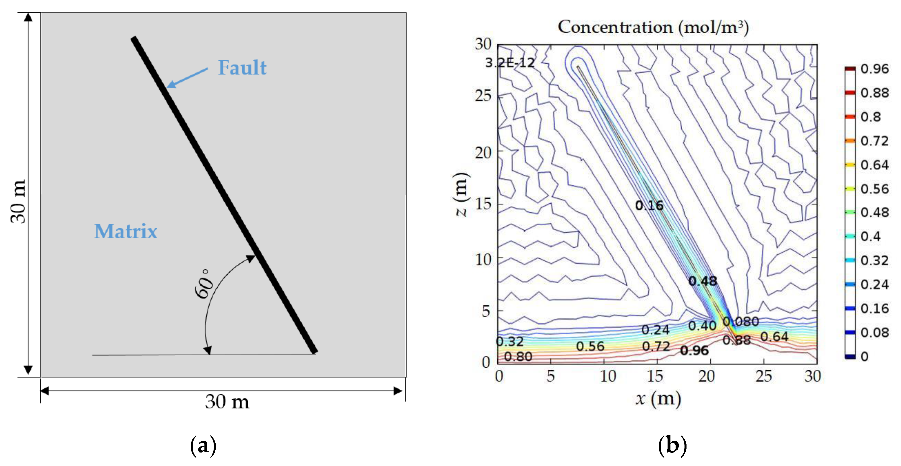
4.1. Geometric Model
4.2. Model Parameters and Properties
4.3. Numerical Results
4.4. Analysis of the Influence Factors on the Water Quality of Aquifers
4.4.1. Existence of NFs and Alkali Erosion
4.4.2. The Effect of the Number of NFs on the Water Quality of Aquifers
4.4.3. The Alkali Erosion on the Water Quality of the Aquifers
5. Conclusions
Author Contributions
Funding
Conflicts of Interest
References
- Kerr, R.A. Natural gas from shale bursts onto the scene. Science 2010, 328, 1624–1626. [Google Scholar] [CrossRef] [PubMed]
- Sun, Z.; Shi, J.T.; Wu, K.L.; Xu, B.X.; Zhang, T.; Chang, Y.C.; Li, X.F. Transport capacity of gas confined in nanoporous ultra-tight gas reservoirs with real gas effect and water storage mechanisms coupling. Int. J. Heat Mass Transf. 2018, 126, 1007–1018. [Google Scholar] [CrossRef]
- Zhang, L.H.; Kou, Z.H.; Wang, H.T.; Zhao, Y.L.; Dejam, M.; Guo, J.J. Performance analysis for a model of a multi-wing hydraulically fractured vertical well in a coalbed methane gas reservoir. J. Pet. Sci. Eng. 2018, 166, 104–120. [Google Scholar] [CrossRef]
- Brantley, S.L.; Yoxtheimer, D.; Arimand, S.; Grieve, P.; Vidic, R.; Pollak, J.; Llewellyn, G.T.; Abad, J.; Simon, C. Water resource impacts during unconventional shale gas development: The Pennsylvania experience. Int. J. Coal Geol. 2014, 126, 140–156. [Google Scholar] [CrossRef]
- King, G.E. Hydraulic fracturing 101: What every representative, environmentalist, regulator, reporter, investor, university researcher, neighbor and engineer should know about estimating fracturing risk. J. Pet. Technol. 2012, 64, 34–42. [Google Scholar] [CrossRef]
- Chermak, J.A.; Schreiber, M.E. Mineralogy and trace element geochemistry of gas shales in the United States: Environmental implications. Int. J. Coal Geol. 2014, 126, 32–44. [Google Scholar] [CrossRef]
- Haluszczak, L.O.; Rose, A.W.; Kump, L.R. Geochemical evaluation of folwback brine from Marcellus gas wells in Pennsylvania, USA. Appl. Geochem. 2013, 28, 55–61. [Google Scholar] [CrossRef]
- Yang, R.D.; Zhang, Y.H.; Gao, J.B.; Wei, H.R.; Su, H.M. Environment impact assessment of shale gas extraction: A case study of the Dawuba formation and Niutitang formation, in Guizhou Provice. Geol. Rev. 2017, 63, 1001–1011. [Google Scholar] [CrossRef]
- You, L.J.; Kang, Y.L.; Chen, Z.X.; Chen, Q.; Yang, B. Wellbore instability in shale gas wells drilled by oil-based fluids. Int. J. Rock Mech. Min. Sci. 2014, 72, 294–299. [Google Scholar] [CrossRef]
- Yu, Y.F.; Kang, Y.L.; Chen, Q.; Yang, B. Alkali corrosion: A new mechanism of shale borehole instability. Acta Pet. Sin. 2013, 34, 983–988. [Google Scholar] [CrossRef]
- Yang, J.; Kang, Y.L.; Lan, L.; Hu, Y.D.; Chen, J.M. Influence of fluid pH on the permeability of tight sandstone reservoir. Nat. Gas Ind. 2005, 25, 33–35. [Google Scholar]
- Li, X.Q.; Hou, D.J.; Tang, Y.J.; Hu, G.Y.; Zhang, A.Y. The preliminary discussion on relationships between chemical compositions of formation fluid and natural gas reservoirs—A case study of central large gas field in Erdos Basin. Fault-Block Oil Gas Field 2002, 9, 1–4. [Google Scholar]
- Wang, X.C.; Zhang, H.L.; Jin, X.P. Analysis and study on the composition of volumetric fracturing flow-back fluid of tight oil in Songliao Basin. Chem. Eng. Eq. 2016, 8, 89–94. [Google Scholar]
- Huang, L.; Li, H.Q.; Yang, P. The components and treatment of shale gas fracturing flowback water. Environ. Sci. Technol. 2016, 39, 166–171. [Google Scholar]
- Ghavami, M.; Hasanzadeh, B.; Zhao, Q.; Javadi, S.; Kebria, D.Y. Experimental study on microstructure and rheological behavior of organobentonite/oil-based drilling fluid. J. Mol. Liq. 2018, 263, 147–157. [Google Scholar] [CrossRef]
- Kang, Y.L.; She, J.P.; Zhang, H.; You, L.J.; Yu, Y.F.; Song, M.G. Alkali erosion of shale by high-pH fluid: Reaction kinetic behaviors and engineering responses. J. Nat. Gas Sci. Eng. 2016, 29, 201–210. [Google Scholar] [CrossRef]
- Birdsell, D.T.; Rajaram, H.; Dempsey, D.; Viswanathan, H.S. Hydraulic fracturing fluid migration in the subsurface: A review and expanded modeling results. Water Resour. Res. 2015, 51, 7159–7188. [Google Scholar] [CrossRef] [Green Version]
- Myers, T. Potential Contaminant Pathways from Hydraulically Fractured Shale to Aquifers. Groundwater 2012, 50, 872–882. [Google Scholar] [CrossRef] [PubMed]
- Gassiat, C.; Gleeson, T.; Lefebvre, R.; McKenzie, J. Hydraulic fracturing in faulted sedimentary basins: Numerical simulation of potential contamination of shallow aquifers over long time scales. Water Resour. Res. 2013, 49, 8310–8327. [Google Scholar] [CrossRef] [Green Version]
- Kissinger, A.; Helmig, R.; Ebigbo, A.; Class, H.; Lange, T.; Sauter, M.; Heitfeld, M.; Klunker, J.; Jahnke, J. Hydraulic fracturing in unconventional gas reservoirs: Risks in the geological system, part 2. Environ. Earth Sci. 2013, 70, 3855–3873. [Google Scholar] [CrossRef]
- Wei, Y.Q.; Dong, Y.H.; Li, G.M. Numerical simulation on the effect of fault on the fracturing fluid migrate. Hydrogeol. Eng. Geol. 2016, 43, 117–123. [Google Scholar] [CrossRef]
- Reagan, M.T.; Moridis, G.J.; Keen, N.D.; Johnson, J.N. Numerical simulation of the environmental impact of hydraulic fracturing of tight/shale gas reservoirs on near-surface groundwater: Background, base cases, shallow reservoirs, short-term gas, and water transport. Water Resour. Res. 2015, 51, 2543–2573. [Google Scholar] [CrossRef] [PubMed] [Green Version]
- Pfunt, H.; Houben, G.; Himmelsbach, T. Numerical modeling of fracking fluid migration through fault zones and fractures in the North German Basin. Hydrogeol. J. 2016, 24, 1343–1358. [Google Scholar] [CrossRef]
- Dejam, M.; Hassanzadeh, H.; Chen, Z.X. Pre-Darcy Flow in Porous Media. Water Resour. Res. 2017, 53, 8187–8210. [Google Scholar] [CrossRef]
- Xu, Y. Theoretical and Numerical Study on Multi-Field Coupling Behavior of Inhomogeneous Model. Master’s Thesis, China University of Mining and Technology, Xuzhou, China, 2014. [Google Scholar]
- Xi, Y.H.; Liu, J.H. Simulation of contaminant migration in saturated porous media. J. Tongji Univ. 2005, 33, 644–648. [Google Scholar]
- Wang, H.T. Dynamics of Fluid Flow and Contaminant Transport in Porous Media, 1st ed.; Higher Education Press: Beijing, China, 2008; pp. 92–94. ISBN 978-7-04-022267-8. [Google Scholar]
- Fang, Z. Theoretical and Experimental Study of Rock Damage Model under Temperature-Mechanical-Chemical Coupling. Master’s Thesis, Central South University, Changsha, China, 2010. [Google Scholar]
- Fusseis, F.; Regenauer-Lieb, K.; Liu, J.; Hough, R.M.; De Cario, F. Creep cavitation can establish a dynamic granular fluid pump in ductile shear zones. Nature 2009, 459, 974–977. [Google Scholar] [CrossRef] [PubMed]
- Kuhl, D.; Bangert, F.; Meschke, G. Coupled chemo-mechanical deterioration of cementitious materials. Part I: Modeling. Int. J. Solids Struct. 2004, 41, 1141–1150. [Google Scholar] [CrossRef]
- Poulet, T.; Karrech, A.; Regenauer-Lieb, K.; Fisher, L.; Schaubs, P. Thermal-hydraulic-mechanical-chemical coupling with damage mechanics using ESCRIPTRT and ABAQUS. Tectonophysics 2011, 124–132. [Google Scholar] [CrossRef]
- McCure, C.C.; Fogler, H.S.; Kline, W.E. An experimental technique for obtaining permeability-porosity relationships in acidized porous media. Ind. Eng. Chem. Fundam. 1979, 18, 188–191. [Google Scholar] [CrossRef]
- Tang, D.H.; Frind, E.O.; Sudicky, E.A. Contaminant Transport in Fractured Porous Media: Analytical Solution for a Single Fracture. Water Resour. Res. 1981, 17, 555–564. [Google Scholar] [CrossRef]
- Zhang, H.X. Production Analysis of Multi-Fractured Horizontal Shale Gas Wells Based on Heterogeneous Model. Master’s Thesis, China University of Mining and Technology, Xuzhou, China, 2017. [Google Scholar]
- Zhou, W.L.; Ma, B.J.; Cheng, L.; Zhang, Y.; Liu, J.; Li, W. Occurrence and risk assessment of heavy metals in Sanmenxia reservoir. Yellow River 2018, 40, 83–87. [Google Scholar] [CrossRef]
- Sui, H.J.; Wu, X.; Cui, Y.S. Modeling heavy metal movement in soil review and further study directions. Trans. CSAE 2006, 22, 197–200. [Google Scholar]
- Liu, Z.G.; Si, C.S.; Shou, J.F.; Ni, C.; Pan, L.Y.; Liu, Q. Origin Mechanism of Anomalous Tightness of Middle and Lower Jurassic Sandstone Reservoirs in Central Sichuan Basin. Acta Sedimentol. Sin. 2011, 29, 744–751. [Google Scholar] [CrossRef]
- Tian, X.; Mao, Z.Q.; Xiao, L.; Zeng, G.; Qian, H.Y. A permeability model built up on low permeability gas reservoirs in Xujiahe formation, Sichuan basin. Nat. Gas Ind. 2009, 29, 39–41. [Google Scholar] [CrossRef]
- Zeng, D.M.; Wang, X.Z.; Zhang, F.; Song, Z.Q.; Zhang, R.X.; Zhu, Y.G.; Li, Y.G. Study on reservoir of the Leikoupo Formation of Middle Triassic in northwestern Sichuan Basin. J. Palaeogeogr. 2007, 9, 253–266. [Google Scholar] [CrossRef]
- Zhang, B.J.; Pei, S.Q.; Yin, H.; Yang, Y. Reservoir characteristics and main controlling factors of Jialingjiang Formation in southwestern Sichuan Basin. Lithol. Reserv. 2011, 23, 80–83. [Google Scholar]
- Fang, L.Z.; Ju, Y.W.; Wang, G.C.; Bu, H.L. Composition and gas-filled pore characteristics of Permian organic shale in southwest Fujian depression, Cathaysia landmass. Earth Sci. Front. 2013, 20, 229–239. [Google Scholar]
- Yang, T.Q.; Mei, Q.; Zhang, H.M.; Li, A.G. Character istics research of Bajiaochang Carboniferous reservoir in Sichuan Basin. Nat. Gas Explor. Dev. 2006, 29, 1–4. [Google Scholar]
- Guo, T.L. Characteristics and exploration potential of Ordovician reservoirs in Sichuan Basin. Oil Gas Geol. 2014, 35, 372–378. [Google Scholar] [CrossRef]
- Shi, S.Y.; Hu, S.Y.; Hong, H.T.; Jiang, H.; Wang, T.S.; Xu, A.N.; Liu, W.; Liu, X.; Zeng, Y.Y.; Chen, W. The characteristics of dolomite reservoir and the prospect of oil and gas exploration in the Cambrian in Sichuan Basin. In Proceedings of the China National Conference of Sedimentology, Jingzhou, China, 24–26 October 2015. [Google Scholar]
- Huang, J.L.; Zou, C.N.; Li, J.Z.; Dong, D.Z.; Wang, S.J.; Wang, S.Q.; Cheng, K.M. Shale gas generation and potential of the Lower Cambrian Qiongzhusi Formation in Southern Sichuan Basin, China. Pet. Explor. Dev. 2012, 39, 69–75. [Google Scholar] [CrossRef]
- Song, J.M.; Liu, S.G.; Li, Z.W.; Luo, P.; Yang, D.; Sun, W.; Peng, H.L.; Yu, Y.Q. Characteristics and controlling factors of microbial carbonate reservoirs in the Upper Sinian Dengying Formation in the Sichuan Basin, China. Oil Gas Geol. 2017, 38, 741–752. [Google Scholar] [CrossRef]


| Contaminants | Contaminated | pH | Composition | Permeable Pathways | References |
|---|---|---|---|---|---|
| Formation Fluid | Yes | 4.0–9.0 | Oil, gas and high-concentration-salt water | Well, fractures or faults | Yang et al. [11] |
| Li et al. [12] | |||||
| Flow-back Fluid | Yes | 7.0–8.0 | Hydraulic Fracturing Fluid and stratigraphic composition | Well, fractures or faults | Wang et al. [13] |
| Huang et al. [14] | |||||
| High-pH Drilling Fluid | Yes | 11.0–12.0 | Diesel or mineral oil with a suspended polymer, synthetic polymer or modified clay | Drilling fluid loss may occur during drilling, and then filtrate may invades into porous formation | Ghavami et al. [15] |
| Kang et al. [16] | |||||
| HF Fluid | Yes | 6.5–7.0 | Water, proppant and chemical additives | Well, fractures or faults | Birdsell et al. [17] |
| Authors | Fluid | Driving Force | Advantages | Disadvantages |
|---|---|---|---|---|
| Myers [18] | HF | imposed at boundaries | Taking the lead in studying the migration of HF fluid and providing ideas for later scholars. | Without consideration of the buoyancy caused by difference in density flow. |
| Gassiat et al. [19] | HF | Reservoir Overpressure | A wide range of parameter studies is presented. | Without consideration of well production. |
| Kissinger et al. [20] | (1), (2): HF fluid and brine; (3): methane | from injection from artesian aquifers (3): Flux from reservoir | Buoyancy is accounted for in all three scenarios and a two-phase model is presented in scenario (3). | (1) and (2) do not consider the effects of imbibition and well production; (3) cannot be used for a quantitative risk analysis. |
| Wei YQ et al. [21] | HF | Buoyancy | The migration of HF caused by density difference is studied in detail. | Without consideration of temperature, alkali erosion and different parameters sensitivity. |
| Reagan et al. [22] | Gas | Buoyancy and well | The effects of multiphase flow, buoyancy and well production on the migration of HF fluid are considered. | Without consideration of NFs and alkali erosion. |
| Birdsell et al. [17] | HF | imposed at boundaries and well | The combination of 5 stages mechanisms is considered and a wide range of parameter studies is presented. | Geological conditions, NFs and alkali erosion are not considered. |
| Pfunt et al. [23] | HF | from injection | The migration of HF caused by density difference is studied in detail. | Without consideration of temperature, alkali erosion and different parameters sensitivity. |
| Parameters | Description | Value |
|---|---|---|
| (kg/m3) | Fracturing fluid density | 1100 |
| (m2) | The matrix permeability in Model 1 | 5.0 × 10⁻¹⁶ |
| (m2) | The upper matrix permeability in Model 2, 3, 4 | 6.0 × 10⁻¹⁶ |
| (m2) | The lower matrix permeability in Model 2, 3, 4 | 4.0 × 10⁻¹⁶ |
| The matrix porosity in Model 1 | 0.1 | |
| The upper matrix porosity in Model 2, 3, 4 | 0.15 | |
| The lower matrix porosity in Model 2, 3, 4 | 0.05 | |
| (m) | Fault width | 0.16 |
| (m) | Fault height | 30 |
| Fault inclination angle | 60 | |
| Fault porosity | 0.2 |
| Heavy Metal Contaminants | Cd | Pb | Co | References |
|---|---|---|---|---|
| Content in flow-back fluid (μg/L) | 689.09 | 10.28 | 200.15 | Yang et al. [8] |
| Water quality standard (μg/L) | ≤1 | ≤10 | Zhou et al. [35] | |
| Risk assessment | Toxic, causing liver or kidney damage easily | Toxic and carcinogenic | Toxic, causing “Carbide disease” | Sui et al. [36] |
| Zone | Stratigraphic Units | Thickness [m] | Porosity | [m]2 | References |
|---|---|---|---|---|---|
| 1 | Cretaceous | 75 | 0.118 | 2.3 × 10⁻¹⁵ | |
| 2 | Jurassic | 400 | 0.05 | 1.0 × 10⁻¹⁵ | Liu et al. [37] |
| 3 | Upper Triassic | 220 | 0.0409 | 1.1 × 10⁻¹⁶ | Tian et al. [38] |
| 4 | Middle Triassic | 250 | 0.0212 | 1.67 × 10⁻¹⁵ | Zeng et al. [39] |
| 5 | Lower Triassic | 650 | 0.025 | 3.5 × 10⁻¹⁶ | Zhang et al. [40] |
| 6 | Upper Permian | 80 | 0.03 | 3.0 × 10⁻¹⁶ | Fang et al. [41] |
| 7 | Lower Permian | 170 | 0.0084 | 8.0 × 10⁻¹⁷ | Fang et al. [41] |
| 8 | Carboniferous | 30 | 0.0203 | 1.0 × 10⁻¹⁵ | Yang et al. [42] |
| 9 | Silurian | 230 | 0.0461 | 1.2 × 10⁻¹⁶ | Fang et al. [41] |
| 10 | Ordovician | 200 | 0.0304 | 2.5 × 10⁻¹⁶ | Guo et al. [43] |
| 11 | Upper Cambrian | 200 | 0.026 | 2.0 × 10⁻¹⁶ | Shi et al. [44] |
| 12 | Middle Cambrian | 160 | 0.0138 | 1.83 × 10⁻¹⁶ | Huang et al. [45] |
| 13 | Weiyuan gas field | 39 | 0.01 | 4.6 × 10⁻¹⁹ | Huang et al. [45] |
| 14 | Lower Cambrian | 96 | 0.021 | 8.0 × 10⁻¹⁷ | Song et al. [46] |
| Parameters | Description | Value |
|---|---|---|
| (m) | Fault width | 10 |
| (m) | Fault height | 2900 |
| Fault inclination angle | 60 | |
| Fault porosity | 0.2 | |
| (kg/m3) | HF fluid density | 1100 |
| The well length | 1500 | |
| (m) | The NFs aperture | 1.0 × 10⁻⁴ |
| (m2/s) | Molecular diffusion coefficient | 1.0 × 10⁻⁹ |
| (m) | Longitudinal dispersivity | 1 |
| (m) | Transversal dispersivity | 0.1 |
| (m2/N) | Compressibility of the matrix | 4.4 × 10⁻¹⁰ |
| (m2/N) | Compressibility of the fluid | 2.4 × 10⁻¹⁰ |
| Case Number | Case 1 | Case 2 | Case 3 |
|---|---|---|---|
| NFs | No | Yes | Yes |
| alkali erosion | No | No | Yes |
| Coefficients | B3 | B2 | B1 | I |
|---|---|---|---|---|
| pH = 11.0 | 5.35894 × 10⁻²⁷ | −5.20613 × 10⁻¹⁹ | 1.65838 × 10⁻¹¹ | −1.11642 × 10⁻⁵ |
| pH = 11.5 | 3.33411 × 10⁻²⁶ | −3.14747 × 10⁻¹⁸ | 9.68256 × 10⁻¹¹ | −5.86163 × 10⁻⁵ |
| pH = 12.0 | 1.97884 × 10⁻²⁴ | −8.47458 × 10⁻¹⁷ | 1.19144 × 10⁻⁹ | −3.76353 × 10⁻⁴ |
| pH = 12.5 | 1.00852 × 10⁻²² | −2.08461 × 10⁻¹⁵ | 1.40358 × 10⁻⁸ | −1.95 × 10⁻³ |
| pH = 13.0 | 5.58023 × 10⁻²¹ | −5.39404 × 10⁻¹⁴ | 1.69686 × 10⁻⁷ | −1.157 × 10⁻² |
© 2018 by the authors. Licensee MDPI, Basel, Switzerland. This article is an open access article distributed under the terms and conditions of the Creative Commons Attribution (CC BY) license (http://creativecommons.org/licenses/by/4.0/).
Share and Cite
Peng, W.; Du, M.; Gao, F.; Dong, X.; Cheng, H. A New Analysis Model for Potential Contamination of a Shallow Aquifer from a Hydraulically-Fractured Shale. Energies 2018, 11, 3010. https://doi.org/10.3390/en11113010
Peng W, Du M, Gao F, Dong X, Cheng H. A New Analysis Model for Potential Contamination of a Shallow Aquifer from a Hydraulically-Fractured Shale. Energies. 2018; 11(11):3010. https://doi.org/10.3390/en11113010
Chicago/Turabian StylePeng, Weihong, Menglin Du, Feng Gao, Xuan Dong, and Hongmei Cheng. 2018. "A New Analysis Model for Potential Contamination of a Shallow Aquifer from a Hydraulically-Fractured Shale" Energies 11, no. 11: 3010. https://doi.org/10.3390/en11113010
APA StylePeng, W., Du, M., Gao, F., Dong, X., & Cheng, H. (2018). A New Analysis Model for Potential Contamination of a Shallow Aquifer from a Hydraulically-Fractured Shale. Energies, 11(11), 3010. https://doi.org/10.3390/en11113010