Multiphysics Modeling for Detailed Analysis of Multi-Layer Lithium-Ion Pouch Cells

Abstract

Multiphysics modeling permits a detailed investigation of complex physical interactions and heterogeneous performance in multiple electro-active layers of a large-format Li-ion cell. For this purpose, a novel 3D multiphysics model with high computational efficiency was developed to investigate detailed multiphysics heterogeneity in different layers of a large-format pouch cell at various discharge rates. This model has spatial distribution and temporal evolution of local electric current density, solid lithium concentration and temperature distributions in different electro-active layers, based on a real pouch cell geometry. Other than previous models, we resolve the discharge processes at various discharge C-rates, analyzing internal inhomogeneity based on multiple electro-active layers of a large-format pouch cell. The results reveal that the strong inhomogeneity in multiple layers at a high C-rate is caused by the large heat generation and poor heat dissipation in the direction through the cell thickness. The thermal inhomogeneity also strongly interacts with the local electrochemical and electric performance in the investigated cell.

1. Introduction

There is a growing demand for advanced energy storage systems. Lithium-ion batteries (LiBs) have become a high-demand energy technology due to their high energy density. As a consequence, they are widely applied in energy storage and supply ranging from electrical vehicles (EVs), hybrid electrical vehicles (HEVs), and small-sized devices in satellites [1,2,3]. However, the need to overcome existing barriers, such as reducing cost and further increasing energy density, motivates the investigation of the impact of macroscopic design features on internal physical processes and their interaction [4]. Those aspects are particularly important in larger-format cells, e.g., pouch cells or cylindrical cells. Such large-format cells are made of multiple layers to achieve high energy density. Therefore, for improvement of large-format cells, it is necessary to deeply investigate a single multi-layer cell, as a detailed insight of heterogeneous multiphysics processes in the cell is helpful for a directed design and optimization of large-format cells.

Mathematical models can be used to describe various coupled physical processes to evaluate their interaction. Such multiphysics models of LiBs can be applied for detailed analysis of internal physical processes and battery performance. Higher dimensional multiphysical models can be used to reveal those aspects in large-format cells and evaluate local heterogeneity for different operating conditions, e.g., charge and environmental temperature.

To establish multiphysics modeling of LiBs, prior studies applied different approaches and coupling methodologies. Several fully coupled 2D electrochemical-thermal models have been developed to investigate multiphysics processes in a special cross-sectioned plane. They are used to analyze the electrochemical effects of current collectors and tabs [5], temperature and current distributions across the battery surface [6,7] and the pseudo-3D porous electrode model for detailed ionic transport [8]. Due to the limitation of model dimensions, these models cannot entirely simulate the real internal physical processes with local heterogeneity. 3D multiphysics modeling of LiBs, with different coupling methods, has been employed to investigate cell multiphysics with 3D cell structures [9,10,11]. However, these papers did not discuss about the influences of electro-active layer numbers and structures on the heterogeneous performance of large-format pouch cells. The discrete structures in large-format cells have a strong effect on battery performance.

For the investigation of battery packs or modules, Guo et al. [12] developed a 3D multiphysics model. This model has been used to study the thermal and electrochemical performance in a module made of three pouch cells. Despite detailed illustration of contour results of electric potential and temperature, the model did not show the internal inhomogeneity of each single cell. Pannala et al. [13] also presented a 3D battery pack model, which was used to simulate all battery components for a detailed evaluation of the thermal and mechanical safety risk under adverse conditions. Although multiphysics modeling of large-format cells has already enabled a detailed investigation of cell components and the impacts of the battery materials on its performance, detailed analysis of inhomogeneous performances in a single large-format pouch cell with multiple electro-active layers was barely addressed. Moreover, to reduce computational cost, internal material homogeneity is often assumed. Therefore, recent multiphysics models provide few results for internal heterogeneity based on electro-active layer structures of a single large-format cell, including dynamic descriptions of such heterogeneous multiphysics processes.

By combining two hierarchical frameworks [14,15] for good management of coupling interfaces and submodel solvers, a 3D multiphysics model is developed for the prediction and investigation of internal inhomogeneity regarding cell structures, which is particularly applicable to large-format pouch cells with multiple electro-active layers. It has been applied for the simulation of a 12 Ah pouch cell with multiple electro-active layers in this paper. Regarding our previous work, this modeling method has already helped us with implementation of a sensitivity analysis work [16]. This model is applied to reveal the thermal-electric-electrochemical interactions and to illustrate local heterogeneous evolutions of physical processes in different layers under various discharge C-rates within the pouch cell. To enable computational efficient simulation, a simplified electrochemical electrode model on electrode level is introduced and coupled to a 3D thermal-electric model on cell level. Meanwhile, the simplified electrochemical model has been successfully validated up to a 4C discharge rate by comparing it to a full-order pseudo-2D (P2D) model [17]. In this work, we will fully introduce our governing equations and geometries of the 3D multiphysics model at first, then the computational framework will be presented and discussed in detail. After a numerical validation of our electrochemical submodel, the thermal-electric-electrochemical simulation results will be displayed and discussed with a special focus on heterogeneity.

2. 3D Multiphysics Model

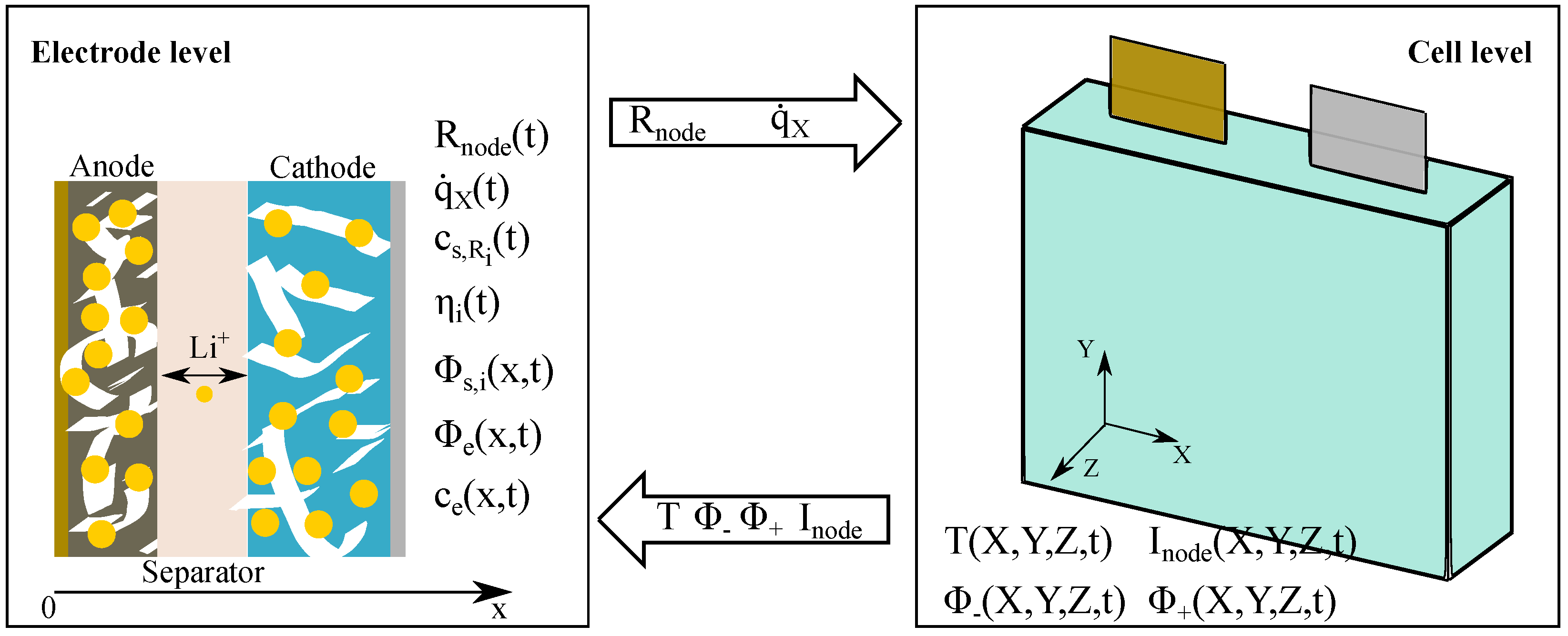
The 3D multiphysics model uses a hierarchical framework to implement the coupling of the different physico-chemical processes within the geometry of the pouch cell presented in this work. The framework and the cell geometry for this 3D model are schematically presented in Figure 1.

The framework consists of two submodels on two levels. These are the electrode and the cell level. On each level, an independent coordinate system is assigned for the discretization. On the electrode level, this coordinate describes the local electrochemical processes of the cell along the x-axis of each electrochemical element, which consists of anode, cathode, separator, and current collectors, in total five computational domains. On the cell level, the cell configuration includes current collector tabs, current collectors, polymer cover, and electro-active layers as computational domains in three dimensions. Each meshed element in an electro-active layer includes all computational domains of the electrode level and is defined as a nonlinear resistor, which represents the local potential drop that stems from the local electrochemical processes. On the cell level, charge and energy conservation equations are solved in three dimensions. Both submodels are coupled by inter-level variables. The submodels and their coupling approach is provided in detail in the following sections.

2.1. Electrode Level: Electrochemical Submodel (ESM)

In the electrochemical submodel (ESM), the electrochemical processes are modeled on the electrode level as shown in Figure 1, based on P2D models [17,18,19]. The discretization in both x and particle radius r directions lead to high computational cost. To reduce the present complexity, two simplifications compared to a full-order P2D model are introduced. In ESM, the pore-wall fluxes $j_{x,i}$ at the electrode-electrolyte interfaces $i=\{cathode,anode\}$ are denoted as average lumped variables over space [20,21]:

$${\overline{j}}_{x,i}=\frac{1}{{\delta }_i}{\int }_{domain:i}{j}_{x,i}\mathrm{d}x,i=ca,an$$

(1)

and it can be calculated according to

$${\overline{j}}_{x,i}=\frac{i_x}{a_{i}F{\delta }_i},$$

(2)

with ${\delta }_i$ electrode thickness, $i_x$ the local current density on the current collector flowing out of the electrode, F the Faraday constant and $a_i$ the specific area of the electrode. The average lumped variable ${\overline{j}}_{x,i}$ simplifies the lithium diffusion process in the active particles, which is usually expressed by Fick’s law:

$$\frac{\partial c_{s,i}}{\partial t}=\frac{1}{r^2}\frac{\partial }{\partial r}\left(r^2{D}_{s,i}\frac{\partial c_{s,i}}{\partial r}\right),$$

(3)

with the boundary conditions of the surface flux at the outer boundary ($r=R_i$) of particles and in the particle center ($r=0$) being given as follows:

$$D_{s,i}\frac{\partial c_{s,i}}{\partial r}{|}_{r=R_i}={\overline{j}}_{x,i}$$

(4)

$$D_{s,i}\frac{\partial c_{s,i}}{\partial r}{|}_{r=0}=0$$

(5)

where $R_i$ is the particle radius and $D_{s,i}$ is the solid diffusion coefficient of the electrode. By taking into account the aforementioned boundary conditions, Equation (3) can be approximately solved as an analytical solution of surface and average lithium concentrations [22]. The surface concentration of lithium in each electrode is expressed as:

$$\begin{array}{cc}\hfill c_{s,surf,i}=& c_{s,init,i}-\frac{3{\overline{j}}_{x,i}t}{R_i}-\hfill \\ & \frac{2{\overline{j}}_{x,i}{R}_i}{D_{s,i}}\left[\left(\frac{1}{10}-\sum _{n=1}^N\frac{1}{{\lambda }_n^2}\right)\left(1-e^{-\frac{{\lambda }_{N+1}{D}_{s,i}t}{R_i^2}}\right)+\sqrt{\frac{D_{s,i}t}{\pi R_i^2}}\mathrm{erfc}\left({\lambda }_{N+1}\sqrt{\frac{D_{s,i}t}{R_i^2}}\right)\right]\hfill \\ & -\sum _{n=1}^N\frac{2{\overline{j}}_{x,i}{R}_i}{{\lambda }_N{D}_{s,i}}\left(1-e^{\frac{-{\lambda }_N^2{D}_{s,i}t}{R_i^2}}\right)\hfill \end{array}$$

(6)

where $c_{s,init,i}$ is the initial lithium concentration in the electrode particle, N is the truncation error term number, and is defined as $N=6$ in this work, and ${\lambda }_n$ is the nth eigenvalue, which can be calculated as follows [22]

$${\lambda }_n-\tan \left({\lambda }_n\right)=0,n=1,2,3,\dots$$

(7)

The bulk concentration in the solid phases ${\overline{c}}_{s,i}$ can be evaluated by solving lumped mass balance:

$$\frac{d{\overline{c}}_{s,i}}{dt}=-3\frac{{\overline{j}}_{x,i}}{R_i},$$

(8)

It is noted that the state of charge (SOC) of the battery is also related to the bulk solid concentration. It is defined by the variation range of bulk solid concentration in cathodes [21], as

$$\mathrm{SOC}=\frac{{\overline{c}}_{s,i}-{\overline{c}}_{s,init,i}}{c_{s,0\%,i}-c_{s,init,i}}.$$

(9)

The initial solid concentration $c_{s,init,i}$ is set as the value when SOC = 100% and the bulk solid concentration at SOC = 0%, $c_{s,0\%,i}$ can be evaluated by

$$c_{s,0\%,i}=c_{s,init,i}+\frac{12\mathrm{Ah}}{N_{layer}{\epsilon }_{s,ca}F{\delta }_{ca}A}.$$

(10)

The solid diffusion overpotential in each electrode ${\eta }_{diff,i}$ is derived as a function of surface and bulk concentrations, and is expressed as:

$${\eta }_{diff,i}=E_i(\frac{c_{s,surf,i}}{c_{s,max,i}})-E_i(\frac{{\overline{c}}_{s,i}}{c_{s,max,i}}),$$

(11)

where $c_{s,max,i}$ is the maximum lithium concentration in active particles, and $E_i$ is the open circuit potential (OCP) in each electrode. The Butler-Volmer equation describes the charge transfer reaction rate at the electrode-electrolyte interfaces. The reaction rate is driven by the kinetic overpotential ${\eta }_{et,i}$, which is defined as the deviation of the potential in solid phase ${\mathsf{\Phi }}_{s,i}$, as well as the potential in the solution phase ${\mathsf{\Phi }}_e$, and $E_i$,

$${\overline{j}}_{x,i}=\frac{i_{0,i}}{a_{i}F}\left[\exp \left(\frac{{\alpha }_{a,i}F{\eta }_{et,i}}{RT}\right)-\exp \left(-\frac{{\alpha }_{c,i}F{\eta }_{et,i}}{RT}\right)\right],$$

(12)

$${\eta }_{et,i}={\mathsf{\Phi }}_{s,i}-{\mathsf{\Phi }}_e-E_i\left(\frac{c_{s,surf,i}}{c_{s,max,i}}\right)$$

(13)

where ${\alpha }_{a,i}$ and ${\alpha }_{c,i}$ are the charge transfer coefficients, R is the ideal gas constant, and $i_{0,i}$ is the exchange current density, which is given as a function of the surface lithium concentration in solid phases and lithium concentration in the solution phase at the electrolyte-electrode interface. (For the evaluation of voltage in ECM element, all field variables, e.g., ${\mathsf{\Phi }}_e,c_e,{\mathsf{\Phi }}_s$, in the anode are evaluated at $x=0$ and in the cathode at $x=L$ [21]).

$$i_{0,i}=k_{0,i}F{c}_e^{{\alpha }_a}{\left(c_{s,max,i}-c_{s,surf,i}\right)}^{{\alpha }_a}{c}_{s,surf,i}^{{\alpha }_c}$$

(14)

Here $k_{0,i}$ is a kinetic rate coefficient, $c_e$ is the lithium concentration in solution phase at the electrolyte-electrode interfaces. Assuming that ${\alpha }_{a,i}={\alpha }_{c,i}=\alpha =0.5$, based on Equation (12), the kinetic overpotential ${\eta }_{et,i}$ can be analytically solved [21]:

$${\eta }_{et,i}=\frac{RT}{\alpha F}\ln \left({\Psi }_i+\sqrt{{\Psi }_i^2+1}\right)$$

(15)

where the term ${\Psi }_i$ is given by Equation (16):

$${\Psi }_i=\frac{R_i{i}_{x}F}{6{\epsilon }_i{i}_{0,an}{\delta }_i},$$

(16)

and ${\epsilon }_i$ is the porosity of electrode i.

For simplification, the voltage in each ESM element can be denoted as the sum of different terms, as described by Prada et al. [21]:

$${\mathsf{\Phi }}_{s,ca}\left(L\right)-{\mathsf{\Phi }}_{s,an}\left(0\right)=E_{ca}\left(\frac{{\overline{c}}_{s,ca}}{c_{s,max,ca}}\right)-E_{an}\left(\frac{{\overline{c}}_{s,an}}{c_{s,max,an}}\right)+{\eta }_{ca}-{\eta }_{an}+{\mathsf{\Phi }}_e\left(L\right)-{\mathsf{\Phi }}_e\left(0\right),$$

(17)

The reference potential on the anode ${\mathsf{\Phi }}_{s,an}\left(0\right)$ is defined by the electric potential at the negative current collector on cell level ${\mathsf{\Phi }}_{-}$. The total overpotential ${\eta }_i$ is defined as the sum of overpotentials of diffusion and kinetics:

$${\eta }_i={\eta }_{diff,i}+{\eta }_{et,i}$$

(18)

The electric potential in electrolyte ${\mathsf{\Phi }}_e$ is evaluated in the continuous liquid phase, which consists of 3 domains, $i=cathode,anode,separator$ at the electrode level:

$$\begin{array}{cc}\hfill \nabla ·\left({\kappa }_i^{eff}\nabla {\mathsf{\Phi }}_e\right)-\nabla \left[\frac{{\kappa }_i^{eff}RT}{F}\left(1+\frac{\mathrm{d}\ln f}{\mathrm{d}\ln c_e}\right)\left(1-t_{+}^0\right)\nabla \ln c_e\right]& +a_{i}F{\overline{j}}_{x,i}=0,\hfill \end{array}$$

(19)

where ${\overline{j}}_{x,sep}=0$. The boundary conditions are given as follows:

$$\nabla {\mathsf{\Phi }}_e{|}_{x=0,L}=0$$

(20)

and at the interfaces,

$$\begin{array}{c}-{\kappa }_{an}^{eff}\nabla {\mathsf{\Phi }}_e{{|}_{x={\delta }_{an}^{-}}=-{\kappa }_{sep}^{eff}\nabla {\mathsf{\Phi }}_e|}_{x={\delta }_{an}^{+}}\hfill \\ -{\kappa }_{sep}^{eff}\nabla {\mathsf{\Phi }}_e{{|}_{x={\left({\delta }_{an}+{\delta }_{sep}\right)}^{-}}=-{\kappa }_{ca}^{eff}\nabla {\mathsf{\Phi }}_e|}_{x={\left({\delta }_{an}+{\delta }_{sep}\right)}^{+}}\hfill \end{array}$$

(21)

where ${\kappa }_i^{eff}$ is the effective ionic conductivity of electrolyte in every domain, $c_e$ is salt concentration in electrolyte and $t_{+}^0$ is the transference number of ${\mathrm{Li}}^{+}$. With Equations (19)–(21), ${\mathsf{\Phi }}_e$ has been calculated analytically in every domain due to the lumped reaction rate as follows [21]:

$${\mathsf{\Phi }}_e\left(x\right)={\mathsf{\Phi }}_e(x=0)+\frac{2RT}{F}\left(1+\frac{\mathrm{d}\ln f}{\mathrm{d}\ln c_e}\right)\left(1-t_{+}^0\right)\ln \frac{c_e\left(x\right)}{c_e(x=0)}-\frac{i_x{x}^2}{2{\delta }_{an}{\kappa }_{an}^{eff}}$$

(22)

for the anode domain,

$${\mathsf{\Phi }}_e\left(x\right)={\mathsf{\Phi }}_e(x=0)+\frac{2RT}{F}\left(1+\frac{\mathrm{d}\ln f}{\mathrm{d}\ln c_e}\right)\left(1-t_{+}^0\right)\ln \frac{c_e\left(x\right)}{c_e(x=0)}-\frac{i_x{\delta }_{an}}{2{\kappa }_{an}^{eff}}-\frac{i_x\left(x-{\delta }_{an}\right)}{{\kappa }_{sep}^{eff}}$$

(23)

for the separator domain, and

$$\begin{array}{c}\hfill {\mathsf{\Phi }}_e\left(x\right)={\mathsf{\Phi }}_e(x=0)+\frac{2RT}{F}\left(1+\frac{\mathrm{d}\ln f}{\mathrm{d}\ln c_e}\right)\left(1-t_{+}^0\right)\ln \frac{c_e\left(x\right)}{c_e(x=0)}+\frac{i_x{\left(L-x\right)}^2}{2{\delta }_{ca}{\kappa }_{ca}^{eff}}\\ \hfill -\frac{i_x}{2}\left(\frac{{\delta }_{an}}{{\kappa }_{an}^{eff}}+2\frac{{\delta }_{sep}}{{\kappa }_{sep}^{eff}}+\frac{{\delta }_{ca}}{{\kappa }_{ca}^{eff}}\right)\end{array}$$

(24)

for the cathode domain. The effective ionic conductivities are defined by ${\kappa }_i^{eff}=\kappa {\epsilon }_i^{brug{g}_i}$, and ${\epsilon }_i$ is the porosity in every domain and $brug{g}_i$ is the Bruggemann coefficient.

The mass conservation of lithium salt in the electrolyte is given by:

$${\epsilon }_i\frac{\partial c_e}{\partial t}=\nabla ·\left(D_{e,i}^{eff}\nabla c_e\right)+\left(1-t_{+}^0\right)a_i{\overline{j}}_{x,i},i=ca,an,sep$$

(25)

with the corresponding boundary conditions expressed by:

$$D_{e,i}^{eff}\nabla c_e{|}_{x=0,L}=0$$

(26)

$$\begin{array}{c}-D_{e,an}^{eff}\nabla c_e{{|}_{x={\delta }_{an}^{-}}=-D_{e,sep}^{eff}\nabla c_e|}_{x={\delta }_{an}^{+}}\hfill \\ -D_{e,sep}^{eff}\nabla c_e{{|}_{x={\left({\delta }_{an}+{\delta }_{sep}\right)}^{-}}=-D_{e,ca}^{eff}\nabla c_e|}_{x={\left({\delta }_{an}+{\delta }_{sep}\right)}^{+}}\hfill \end{array}$$

(27)

Here, $D_{e,i}^{eff}$ is the effective diffusion coefficient of electrolyte, which is evaluated by $D_{e,i}^{eff}=D_e{\epsilon }_i^{brug{g}_i}$ for every domain. The governing equations of the electrochemical submodel, all summarized parameters and material properties of the ESM are listed in Appendix A and Appendix B, respectively. Further equations about temperature dependence and thermal behavior are given in the following sections.

2.2. Thermal-Electric Submodel

On the cell level, a 3D thermal-electric continuum submodel is developed to solve temperature T, and local electric potentials ${\mathsf{\Phi }}_{+}$ and ${\mathsf{\Phi }}_{-}$ at the current collectors and tabs. A 3D geometry of a lithium-ion pouch cell with multiple electro-active layers is considered to be illustrated in Figure 1. It consists of 6 computational domains—two electric tabs, two electric current collectors, electro-active layers, and polymer cover. There are 40 parallel layers in the electro-active domain. The heat convection boundary conditions are set on the domains of polymer cover and tabs. Thermal and electric properties of cell components are considered to be anisotropic in the XY-plane and in Z-directions [7]. The energy conservation for all domains yields:

$$\rho C_p\frac{\partial T}{\partial t}=\nabla ·\left(\lambda \nabla T\right)+{\dot{q}}_X,$$

(28)

where the material density of cell component $\rho$, specific heat capacity $C_p$ and thermal conductivity $\lambda$ are attributed to every domain. The volumetric heat source in the electro-active domain ${\dot{q}}_X$ is the sum of the reaction heat ${\dot{q}}_{X,r}$, the entropy change ${\dot{q}}_{X,S}$ and Joule heat ${\dot{q}}_{X,\mathsf{\Omega }}$:

$${\dot{q}}_X={\dot{q}}_{X,r}+{\dot{q}}_{X,\mathsf{\Omega }}+{\dot{q}}_{X,S}.$$

(29)

All locally volumetric heat sources are determined by the electrochemical submodel on the electrode level. The coupling values and expressions will be introduced in the following section. In present simulation scenarios, the cell surfaces are assumed to be exposed to the environment, where the convective heat transfer boundary conditions on surfaces including tabs yield:

$$-\overrightarrow{n}·\lambda \nabla T={\alpha }_h(T-T_{amb}),$$

(30)

where $\overrightarrow{n}$ is the normal unit vector, $T_{amb}$ is constant ambient temperature and ${\alpha }_h$ is the heat transfer coefficient between cell and the environment. The charge conservation of the cell follows Ohm’s law. In tab and current collector domains, it is expressed as:

$$\nabla ·\left({\sigma }_j\nabla {\mathsf{\Phi }}_j\right)+i_X=0,j=-,+$$

(31)

where ${\sigma }_j$ is the electrical conductivity of electrode current collector (+ or −), and $i_X$ is the volumetric current density flowing from electro-active layers. In tab domains, $i_X$ is zero. For a discharge process, the electric boundary conditions as shown in Figure 1 are expressed as

$$\overrightarrow{n}·\left(-{\sigma }_{-}\nabla {\mathsf{\Phi }}_{-}\right)=\frac{I}{A_{-}}$$

(32)

at the negative electrode tab, and

$$\overrightarrow{n}·\left(-{\sigma }_{+}\nabla {\mathsf{\Phi }}_{+}\right)=-\frac{I}{A_{+}}$$

(33)

at the positive electrode tab, where $A_{-}$ and $A_{+}$ are areas of anode and cathode tabs, respectively. On the tab terminal of anode current collectors, the reference potential is defined as:

$${\mathsf{\Phi }}_{-}=0$$

(34)

A 1D nonlinear resistor network is employed for charge conservation in electro-active domain instead of Poisson’s equation in Z-direction [23]. The number of nonlinear resistors $N_e$ is equal to the number of nodes on the XY-plane after meshing the cell (see Figure 1). According to Gerver’s approach [23], the local current $I_{node}$ in the electro-active domain follows the relation:

$$I_{node}=\frac{{\mathsf{\Phi }}_{+,node}-{\mathsf{\Phi }}_{-,node}}{R_{node}}$$

(35)

where ${\mathsf{\Phi }}_{+,node}$ and ${\mathsf{\Phi }}_{-,node}$ are the local potentials at nodes on cathode and anode current collectors on the XY-plane, respectively. $R_{node}(I_{node},{\eta }_{node})$ is the local resistance evaluated by an independent electrochemical submodel. Using nonlinear resistors, it is possible to combine local electrochemical processes with geometry on the cell level. Therefore, the coupling of too many partial differential equations (PDEs) of electrochemical processes is avoided, and the simulation of charge conservation in 3D pouch cell configuration with a faster convergence than full-physics coupling is enabled [23].

2.3. Model Coupling

Figure 1 shows the coupling of the two submodels. Each independent electrochemical submodel performs as a nonlinear resistor on cell level. In the following we will introduce the coupling strategy between both level submodels and the computational framework.

2.3.1. Inter-Level Coupling Variables

In this 3D multiphysics model, variables on the electrode level are firstly solved, then these solutions are delivered to the cell level through inter-level coupling variables as shown in Figure 2. In the electrochemical model, local resistance $R_{node}(X,Y,Z)$ and volumetric heat source ${\dot{q}}_X(X,Y,Z)$ are determined. The thermal-electric submodel provides local temperature $T(X,Y,Z)$, electric potentials ${\mathsf{\Phi }}_{+}(X,Y,Z)$ and ${\mathsf{\Phi }}_{-}(X,Y,Z)$, and local current $I_{node}(X,Y,Z)$ as an input for the electrochemical submodels. The local temperature of an electro-active element is the average value of its corresponding nodes. The local resistance $R_{node}$ is defined as a function of local current $I_{node}$ and local potential drop between anode and cathode current collectors. The potential drop is coupled on both levels:

$${\mathsf{\Phi }}_{+,node}-{\mathsf{\Phi }}_{-,node}={\mathsf{\Phi }}_{s,ca}\left(L\right)-{\mathsf{\Phi }}_{s,an}\left(0\right)$$

(36)

Then using Equations (15)–(17), (22) and (24), this potential drop can be finally written as:

$$\begin{array}{cc}\hfill {\mathsf{\Phi }}_{+,node}-{\mathsf{\Phi }}_{-,node}=& E_{ca}\left({\theta }_{ca}\right)-E_{an}\left({\theta }_{an}\right)\hfill \\ & +\frac{RT}{\alpha F}\ln \left(\frac{{\Psi }_{ca}+\sqrt{{\Psi }_{ca}^2+1}}{{\Psi }_{an}+\sqrt{{\Psi }_{an}^2+1}}\right)\hfill \\ & +\frac{2RT}{F}\left(1+\frac{\mathrm{d}\ln f}{\mathrm{d}\ln c_e}\right)\left(1-t_{+}^0\right)\ln \frac{c_e\left(L\right)}{c_e\left(0\right)}\hfill \\ & -\frac{i_x}{2}\left(\frac{{\delta }_{an}}{{\kappa }_{an}^{eff}}+2\frac{{\delta }_{sep}}{{\kappa }_{sep}^{eff}}+\frac{{\delta }_{ca}}{{\kappa }_{ca}^{eff}}\right).\hfill \end{array}$$

(37)

where ${\theta }_i=c_{s,surf,i}/c_{s,max,i}$. $I_{node}$ is a local current of the corresponding resistor and is denoted by:

$$I_{node}=\frac{i_{x}A}{N_{elem}}$$

(38)

where $N_{elem}$ is the total number of electrochemical submodel elements in an electro-active layer.

Using a similar approach for the coupling of electrochemical processes and charge conservation on both levels, the volumetric heat sources ${\dot{q}}_{X,r}$, ${\dot{q}}_{X,\mathsf{\Omega }}$ and ${\dot{q}}_{X,S}$ are defined as average values on electrode level as follows [24]:

$${\dot{q}}_{X,r}=\sum _{i=ca,an}{a}_{i}F{\overline{j}}_{x,i}{\eta }_i,$$

(39)

$${\dot{q}}_{X,\mathsf{\Omega }}=a_{i}F{\overline{j}}_{x,i}\left[{\mathsf{\Phi }}_e\left(L\right)-{\mathsf{\Phi }}_e\left(0\right)\right]$$

(40)

and

$${\dot{q}}_{X,S}=\sum _{i=ca,an}{a}_{i}F{\overline{j}}_{x,i}T\frac{\partial E_i}{\partial T}$$

(41)

Using the three terms above, the volumetric heat source ${\dot{q}}_X$ of every corresponding node in the resistor element can be evaluated by Equation (29). For example, if the resistor is a linear element with two nodes, then one node represents the anode, and the other one denotes the cathode. Also, every volumetric heat source is divided into two pieces: anode and cathode, and then they are assigned accordingly. For the ohmic heat loss, it is assumed that the active material is well electronically conductive, thus the ohmic loss in solid phases is neglected here.

2.3.2. Computational Framework

Referring to Allu’s [14] and Kim’s [15] works, the framework of the 3D multiphysics model with the inter-level coupling variables enables different solvers to be deployed with the different submodels. Figure 3 illustrates the coupling algorithm in detail.

The 3D multiphysics diagram shows that the electrochemical submodel provides and calculates nodal and elemental electrochemical information ${\dot{q}}_X$ and $R_{node}$ in the electro-active domain on the cell level, and the 3D cell-level submodel provides averaged lumped inputs T, ${\mathsf{\Phi }}_j$ and $I_{node}$ for the electrode-level model. At the beginning of each simulation, on both electrode and cell levels, initial conditions are evaluated by static calculations of the two submodels. After starting the transient simulation, at the start of any time step, $t_i$, all stored solutions and inter-level coupling variables on both levels are defined by the recent state at $t_i$. The meshing resolution and the number of nodes in the electro-active domain determine the total number of electrochemical submodels. All electrochemical submodels read their inter-level coupling variables from the 3D thermal-electric submodel and calculate the following states at $t_{i+1}$ with a self-consistent iteration. Consequently, the exchange state of all corresponding electrochemical submodels at $t_{i+1}$ and the recent state of the 3D submodel at $t_i$ are employed in the 3D thermal-electric submodel to calculate its new exchange states at $t_{i+1}$. At the end of this iterative process, new exchange states of both submodels become the recent states, and the 3D multiphysics model continues with the next global time step. This iterative approach of the 3D multiphysics model is based on Picard iterative method, which has been used for transient calculation of multiphysics models. It enables each submodel to proceed with its own self-consistent iterations to reach a convergence criterion after each global time step is increased [14].

2.4. Model Studies

In this paper, the electrochemical submodel is validated first at various current rates with a full-order P2D model [17], then the 3D multiphysics model is used to simulate a 12 Ah large-format pouch cell at various discharge rates under galvanostatic discharge conditions. The electrodes of the cell are composed of lithium rich NCM materials (Ni, Co, Mn) and graphite, respectively. We assume a binary electrolyte containing ${\mathrm{LiPF}}_6$ in ethylene carbonate/ethyl methyl carbonate. The cell properties are presented in the Appendix B and Appendix C as model parameters. The cell dimensions were 99 mm width × 120 mm height × 9 mm thickness. The cell contains 40 parallel stacked electro-active layers, regarding the normal number of layers for commercial pouch cell [12]. The multiphysics model was defined as an open system, with a convective heat exchange coefficient of 15 $\mathrm{W}/{\mathrm{m}}^2·\mathrm{K}$ connected to the environment. The initial and ambient temperatures were chosen as 25 ${}^{\circ }\mathrm{C}$. The electrochemical submodels were implemented in MATLAB (R2015b, MathWorks, Natick, MA, USA) with SundialsTB solvers [25]. The computation cost of electrochemical submodels is estimated by MATLAB using the function tic-toc; it can record the internal execution time for MATLAB programs. The 3D thermal-electric submodel was implemented in Ansys APDL 15.0. All simulations were executed on an 8 core I7-2600 processor with 16 GB memory.

3. Results and Discussion

3.1. Numerical Validation of Electrochemical Submodel

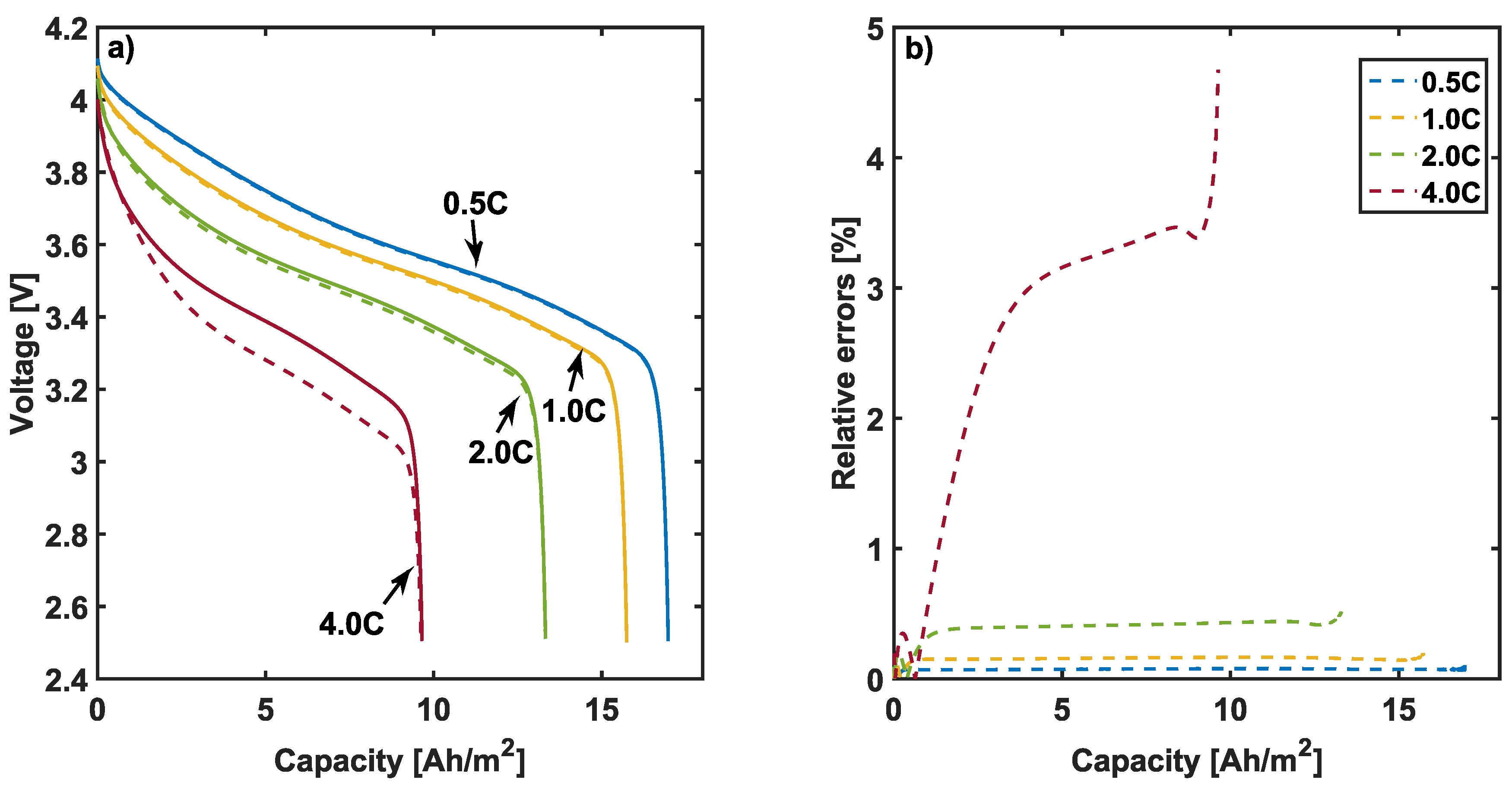
The ESM is validated by comparing the discharge behavior for multiple C-rates to a full-order P2D model [17] as shown in Figure 4.

Figure 4a illustrates that the discharge curve of ESM is in good agreement with the full-order P2D model below 4C discharge, but it shows a larger deviation at 4C. The relative error of ESM at 4C for discharge voltage nearly increases to $5\%$ in the end as shown in Figure 4b. For the simulation carried out in this work, this error is still within an acceptable range, because it does not lead to large deviations of inter-level coupling variables for the multiphysics model. The deviation is likely caused by the assumption of lumped pore-wall flux, which results in overestimated reaction rates along the anode. As a consequence, ESM overestimates the consumption of Li${}^{+}$ at the anode and leading to higher overpotentials. Nevertheless, the final capacity is identical, which suggests that the entire process is not affected by this overestimation.

This observed deviation in voltage curves is further evaluated in Figure 5, where salt concentrations in the electrolyte are shown. The electrolyte salt concentration distribution in ESM is consistent with the results of the P2D model at 1C, but differs at 4C discharge after 10 s. The electrolyte salt concentration decreases faster in the anode domain in ESM. The salt concentration in electrode domains is related to the local electrochemical reaction rates, which originate from the pore-wall fluxes at electrode-electrolyte interfaces. In ESM, the pore-wall flux is assumed to be constant along x-direction as shown in Figure 1. In contrast, in the P2D model fluxes are higher close to the separator. Therefore, the assumption of the lumped reaction rate overestimates potential losses on the simulation of discharge behavior from full-order model at very high C-rates. To conclude, ESM model is sufficiently accurate below discharge rates of 4C but should be replaced with the full-order P2D model at higher rates. However, ESM is computationally much more efficient compared to the full-order P2D model, as evaluated in

Table 1. Computational cost of simulating discharge processes at different C-rates under galvanostatic conditions, using electrochemical submodel (ESM) and pseudo-2D (P2D) model.

	0.5C	1.0C	2.0C	4.0C
ESM	9.21 s	9.46 s	7.31 s	5.80 s
P2D	39.80 s	50.19 s	39.22 s	33.63 s

.

Therefore, ESM can considerably reduce the computational cost with a moderate reduction of accuracy at appropriate C-rate ranges. This is particularly relevant for applications which involve 3D multiphysics simulation due to the parallel executions of a very large number of ESMs.

3.2. Temperature Distribution

Temperature distribution at the end of discharge is shown in Figure 6 for the investigated cell, both on the surface and on cross-sectional area in the center of the electro-active layers for 1C and 4C discharge.

When comparing surface and central temperature distribution at 1C and 4C discharge, it can be seen that temperature distribution is more uniform on the surface at 1C discharge rate. For the cell interior in all C-rate cases, temperature on XY-planes distributes more homogeneously than the temperature distributes along Z-direction, i.e., between center and the surface. This is caused by the low heat conductivity of the electro-active layers along Z-direction. Therefore, the poor heat dissipation through the cell and convective boundaries on the cell surfaces result in higher temperature gradients in the cell center. As shown in Figure 6b,d, the local temperature near the tabs appear higher than on other places in the cell center. Firstly, the tabs are the places that converge and distribute the cell current. These obtain a larger current density than on other places, thereby generating more heat. Secondly, the tabs connect the current collectors. Both are good heat conductors. Due to the increased heat generation in the cell center, the current collectors conduct more heat to the tabs. Therefore, the area near the tabs in the cell center show higher temperatures than other positions. This similar phenomenon has also been observed by others with different cell configurations [12,15]. However, their models did not illustrate the discrete structure and inhomogeneity of the electro-active layers. Our model considers this aspect of thermal inhomogeneity in the electro-active layers and our simulations reveal the temperature evolutions, as demonstrated in the following.

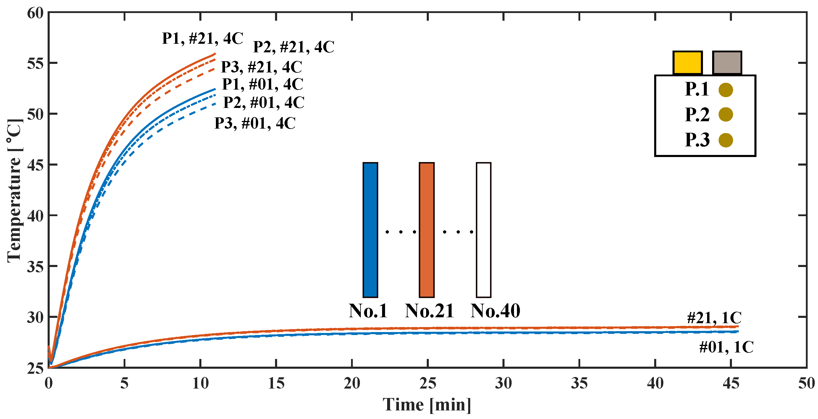
The evolution of local temperature on both surface and central layers is analyzed with Figure 7. The surface and the central layers are represented by layer No.1 and No.21, respectively. Furthermore, the temperature is evaluated at various positions within one layer as P1, position close to the tab, P2, central position, and P3, position far from the tab, as displayed in the inset of Figure 7. As shown previously, the temperature difference between surface and center is considerably compared to temperature difference within a single layer. The maximum temperature difference between layer No.1 and No.21 reaches 4.94 ${}^{\circ }$C at the end of 4C. However, with 1C discharge, only a small temperature difference between these two layers can be observed.

This result indicates that particularly the lower heat conductivity along Z-direction can lead to non-uniform temperature distributions through Z-direction. However, at higher C-rates, a considerable temperature gradient is also observed on the XY-plane. It stems from the current density distribution on the XY-plane, since the thermal conductivities on XY-plane are much higher. The heat which generated from local currents leads to a significant thermal heterogeneity through and across the electro-active layers at the 4C discharge. Waldmann et al. [26] have observed similar results of thermal behavior of the cell surface for large-format Li-ion cells, in their experimental operando studies. With the limitation of the thermal camera, the tests cannot observe the heterogeneity inside the cells. Our model supplements such lack of the cell internal analysis of heterogeneous thermal behavior for advanced cell design.

3.3. Current Density Distribution

Figure 8 shows the electric current density $i_X(X,Y,Z)$ distribution on copper current collectors of different layers, at 1C and 4C discharge at $SOC=50\%$.

As can be seen in Figure 8a, the current density at 1C is larger near the tabs of layer No.1 compared with Figure 8b. In contrast, at 4C, the largest local current density appears near the tabs of layer No.21 at 4C as shown in Figure 8c,d. Figure 8c,d present larger gradients of current density on both layer No.1 and No.21 at 4C, which are consistent with the thermal contours shown in Figure 6. The uniform temperature distribution across electro-active layers at 1C indicates that the local temperature is not the major cause for uneven current density distribution in the case of low applied current. It is mainly influenced by electrostatic potential, which changes quickly near the tabs [15]. In contrast, when discharging with 4C, since local temperatures increase quickly, the thermal effects become significant. Higher temperature is beneficial for the electron-transfer reactions. Local resistance $R_{node}$ in Equations (35) and (37) is related to electrochemical reaction kinetics. The local resistance $R_{node}$ along the Z-direction decreases when local temperature is increasing. The local temperature on layer No.21 is higher than on layer No.1 and forms a considerable temperature gradient within a single layer, and thus, the local resistance on layer No.21 is smaller than other layers. This finally results in higher local current density on this layer. Additionally, a larger current density gradient is visible, which is caused by the higher local temperature and larger temperature gradients. Thereby, this result suggests that the internal current density prefers to travel from anode to cathode in a shorter route at high C-rates in central layers of the large-format cell due to the higher local temperature.

Despite the relation between local temperature and current density, the evolution of local current density shows a significantly more complex, non-monotonic behavior than temperature suggests, which is shown in Figure 9. Here, the evolution of locally produced current density is shown at position P1, P2 and P3 in layer No.1 and No.21 at both 1C and 4C discharge rates.

As can be seen in Figure 9a, local current density on the chosen positions of layer No.1 and No.21 is close to the nominal current density of $25.25\mathrm{A}/{\mathrm{m}}^2$ during 1C discharge process. Due to the fast electrostatic potential change near tabs as mentioned before, the value of local current density is above the nominal value on the positions close to the tabs. It indicates that the stored Li in the region close to the tabs is preferentially consumed. Please note that the initial value of the current density on layer No.1 is larger than the same position on layer No.21, this is because the finite number of tabs and the tab positions can result in a non-uniform current density distribution among multiple layers or rolls [27]. The dynamical change of local current density stems from local resistance variation. As inferred in Equation (14), the local resistance is derived from thermodynamic status, lithium transport in solid and liquid phases and kinetics. At 1C discharge, due to smooth transport processes, the local resistance is sensitive to SOC or the depth of solid lithium intercalation, which is related to its kinetics and thermodynamic status. Since P1 on both layers and P2 on layer No.1 react faster initially with higher local current densities, deeper deintercalation leads to smaller SOC, larger overpotential, and finally larger local resistance. As a consequence, the local current density on these positions decreases during discharge, and the local current density on P3 of both layers retains a constant value during discharge, and at the end, gradually increases to the nominal value due to slight temperature increasing from cell heating. This effect is also mentioned by Lee et al. [27]. This heterogeneity drives temporal variation of current density distributions. The balance between cells is based on the driving force from the sensitive relationship between SOC or depth of discharge and thermodynamic status and diffusion reflected by overpotential [15]. By the end of the discharge process, this relation becomes much more sensitive. Only slight local SOC stemming from larger local current densities results in much larger local resistance. As a consequence, the local current densities on these positions decrease rapidly, and local current densities on other positions increase quickly due to smaller local resistance.

Similar interactions are illustrated at 4C as shown in Figure 9b. It also depicts considerable differences of current density between layer No.1 and No.21 at 4C. As mentioned above, the finite tab number and the different distance to the tabs result in a non-uniformly spatial current density distribution at the beginning of discharge. The local values on layer No.1 are large initially. Afterwards, based on larger local current density, SOC on layer No.1 decreases faster, resulting in larger local resistance. Meanwhile, the temperature in layer No.21 increases rapidly due to cell heating, driving faster local kinetics, which results in smaller local resistance. Consequently, this heterogeneity causes a rapid decrease of current density on layer No.1 and increase on layer No.21 in the first 2 min. Then the local performance is determined significantly by thermal effects. As the local temperatures in the region close to the tabs are much higher than at other positions as shown in Figure 6, the local resistance in this region becomes much smaller. The local current density on P1 of layer No.01 and No.21 keeps increasing. The evolutions on other positions are affected by the interaction of thermal effects and thermodynamic status as well, but also by transport limitations. The temporal variations of local SOC and temperature determines current density evolution during 4C discharge. At the end of the 4C discharge, the local current density is controlled by SOC, i.e., the depth of discharge. Here, similar to the 1C discharge, the region with higher current density decreases rapidly, and vice versa. The complex evolution at 4C reveals that the electric current density at high C-rates is strongly affected by thermal effects. During the discharge process, the spatial and temporal variations of current density in the cell is gradually determined by the interaction of thermal effects and SOC. Due to a much more sensitive relation between SOC and local resistance, as a consequence, the local current density is mainly controlled by SOC, reflecting thermodynamic status and diffusion limitations. The local current densities on different electro-active layers show a strong electric heterogeneity, which also affects the electrochemical heterogeneity considering reactions and phase changes in the active materials.

3.4. The Solid Lithium Concentration Distribution

Local distributions of the relative average solid lithium concentration ${\overline{\theta }}_{an}$ in the anode at different layers are displayed in Figure 10.

It can be seen that there is a positive gradient of solid lithium concentration from the tabs to the bottom of the cell, which is similar, but in the opposite direction of the current density distribution shown previously. This is expected as the local current density determines the local reaction rate, and thus, the local intercalation fraction. Therefore, in accordance with the respective current density, as shown in Figure 8 and Figure 9, the lowest concentration of lithium in the solid of anode active material appears near the tabs of layer No.1 at 1C and layer No.21 at 4C.The wider range of solid lithium concentration denotes a stronger heterogeneity of lithium accumulation in the electro-active layers at 4C, and compared with the results of the temperature and current density contours in Figure 6 and Figure 8. It illustrates that thermal and electric factors in the cell have joint effects on the electrochemical performance in electro-active layers.

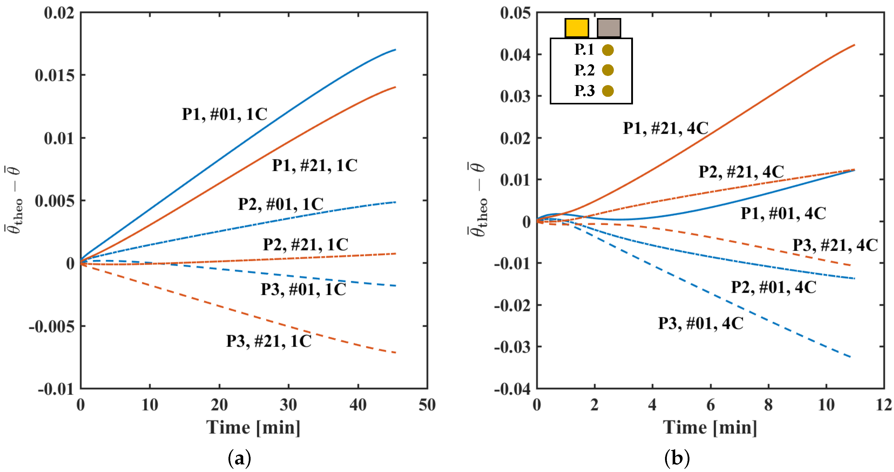
The time dependence of solid lithium concentration evolution also presents such interactions, as Figure 11 demonstrates. We evaluate the same positions which are used for local variations in temperature and electric current density. The concentration evolution is displayed as a difference to the theoretical average value ${\overline{\theta }}_{theo}$ calculated by Faraday’s law, as follows:

$$\frac{\partial {\overline{\theta }}_{theo}}{\partial t}=\frac{i_{x,nom}\ast N_{rate}}{F{\delta }_{an}{c}_{s,max,an}}$$

(42)

As shown in Figure 11a, the local lithium concentration at P1 in layer No.1 is lower than at all other positions at 1C. This corresponds with its highest current density illustrated in Figure 9a. For the positions with smaller current density than the nominal value, the reaction rates are slower than the theoretical average value. Due to the deviation from average current density, all positions perform differently from the theoretical average value during 1C discharge. Figure 11b reveals a more complex solid concentration variation at 4C. Due to higher local resistance at the beginning, P1 on layer No.1 reacts slower than the average with a smaller current density. Then the smaller solid lithium concentration in the center shifts the local thermodynamic equilibrium, resulting in an increase of local resistance. The current density on P1 of layer No.1 gradually increases, and thus the solid lithium concentration on P1 of layer No.1 gradually decreases faster than the theoretical average value at 4C. As expected, the heterogeneity of the local solid concentration is much stronger at 4C than that of 1C, as shown in Figure 11. Paxton et al. [28] experimentally tracked such heterogeneity in 8 Ah ${\mathrm{LiFePO}}_4$ cells, and they found that the cell interior had uneven discharge behavior. They obtained similar observations of solid concentration mapping and evolution, when compared to our model simulation results.

The results for solid lithium concentration confirm that thermal, electric, and electrochemical performances in the cell are strongly interacting during discharge processes. Especially at high C-rates, the main determining factors of battery performance can vary dynamically depending on local temperature and cell design, with changing local physical states. This is essential information for designing large-format cells for high power and energy.

4. Conclusions

In this paper, an efficient 3D multiphysics model was developed for investigating physical interactions and heterogeneity of a 12 Ah large-format pouch cell. It couples local electrochemical submodels with a 3D thermal-electric submodel. The simplified electrochemical submodel was validated against a P2D model up to 4C discharge rate. Analyzing a 12 Ah pouch cell, the following can be concluded:

• At low discharge C-rates, cell temperature is uniformly distributed and has only a few impacts on the behavior of local electric current density and electrochemical reactions, whereas at high discharge C-rates, cell performance is strongly affected by its thermal behavior, leading to heterogeneity of temperature distribution, electric current density and solid lithium concentration in different electro-active layers.
• The local current density at the current collectors is mainly affected by the electrostatic potential at low C-rates. Electrochemical performance at high C-rates are evidently interacting with local current density and thermal effects. The largest local current density always appears near the tabs of the cell.
• During discharge, the different locations in the cell are exposed to different magnitudes of current, heat generation and state of charge. It affirms that our 3D multiphysics model can successfully investigate the effects of cell configurations and components on internal multiphysics. Furthermore, the results at high C-rates suggest that cells that are subjected to such high currents should be optimized for more homogeneous temperature distribution and heat removal, e.g., via changing cell structure or heat dissipation methods. Furthermore, the inhomogeneity in temperature and performance should be taken into account when analyzing such cells, e.g., by experimentally adding more sensors.

Knowing the state of large-format Li-ion batteries is essential for safe and high-performance operations. The 3D multiphysics model revealed highly complex, non-intuitive behavior and interactions with heterogeneously local dynamic behavior in a large pouch cell, which cannot be reproduced with only a homogeneous 3D-thermal-electrical model or with 2D models, as the complex behavior will affect performance lifetime and safety of such cells. This 3D multiphysics model, regarding its detailed interpretations of multiphysics heterogeneity in large-format cells with real geometries, has a great potential in the area of cell design for different real geometries, cell optimization and battery management systems.

References

- Karden, E.; Ploumen, S.; Fricke, B.; Miller, T.; Snyder, K. Energy storage devices for future hybrid electric vehicles. J. Power Sources 2007, 168, 2–11. [Google Scholar] [CrossRef]
- Lu, L.; Han, X.; Li, J.; Hua, J.; Ouyang, M. A review on the key issues for lithium-ion battery management in electric vehicles. J. Power Sources 2013, 226, 272–288. [Google Scholar] [CrossRef]
- Brown, S.; Ogawa, K.; Kumeuchi, Y.; Enomoto, S.; Uno, M.; Saito, H.; Sone, Y.; Abraham, D.; Lindbergh, G. Cycle life evaluation of 3Ah LixMn2O4-based lithium-ion secondary cells for low-earth-orbit satellites. J. Power Sources 2008, 185, 1444–1453. [Google Scholar] [CrossRef]
- Li, J.; Du, Z.; Ruther, R.E.; AN, S.J.; David, L.A.; Hays, K.; Wood, M.; Phillip, N.D.; Sheng, Y.; Mao, C.; et al. Toward Low-Cost, High-Energy Density, and High-Power Density Lithium-Ion Batteries. JOM 2017, 69, 1484–1496. [Google Scholar] [CrossRef] [Green Version]
- Xu, M.; Zhang, Z.; Wang, X.; Jia, L.; Yang, L. Two-dimensional electrochemical–thermal coupled modeling of cylindrical LiFePO4 batteries. J. Power Sources 2014, 256, 233–243. [Google Scholar] [CrossRef]
- Samba, A.; Omar, N.; Gualous, H.; Firouz, Y.; Van den Bossche, P.; Van Mierlo, J.; Boubekeur, T.I. Development of an Advanced Two-Dimensional Thermal Model for Large size Lithium-ion Pouch Cells. Electrochim. Acta 2014, 117, 246–254. [Google Scholar] [CrossRef]
- Tourani, A.; White, P.; Ivey, P. A multi scale multi-dimensional thermo electrochemical modelling of high capacity lithium-ion cells. J. Power Sources 2014, 255, 360–367. [Google Scholar] [CrossRef]
- Northrop, P.W.C.; Pathak, M.; Rife, D.; De, S.; Santhanagopalan, S.; Subramanian, V.R. Efficient Simulation and Model Reformulation of Two-Dimensional Electrochemical Thermal Behavior of Lithium-Ion Batteries. J. Electrochem. Soc. 2015, 162, 940–951. [Google Scholar] [CrossRef]
- Wu, B.; Li, Z.; Zhang, J. Thermal Design for the Pouch-Type Large-Format Lithium-Ion Batteries: I. Thermo-Electrical Modeling and Origins of Temperature Non-Uniformity. J. Electrochem. Soc. 2014, 162, A181–A191. [Google Scholar] [CrossRef]
- Samba, A.; Omar, N.; Gualous, H.; Capron, O.; Van den Bossche, P.; Van Mierlo, J. Impact of Tab Location on Large Format Lithium-Ion Pouch Cell Based on Fully Coupled Tree-Dimensional Electrochemical-Thermal Modeling. Electrochim. Acta 2014, 147, 319–329. [Google Scholar] [CrossRef]
- Xu, M.; Zhang, Z.; Wang, X.; Jia, L.; Yang, L. A pseudo three-dimensional electrochemical–thermal model of a prismatic LiFePO4 battery during discharge process. Energy 2015, 80, 303–317. [Google Scholar] [CrossRef]
- Guo, M.; Kim, G.H.; White, R.E. A three-dimensional multi-physics model for a Li-ion battery. J. Power Sources 2013, 240, 80–94. [Google Scholar] [CrossRef]
- Pannala, S.; Turner, J.A.; Allu, S.; Elwasif, W.R.; Kalnaus, S.; Simunovic, S.; Kumar, A.; Billings, J.J.; Wang, H.; Nanda, J. Multiscale modeling and characterization for performance and safety of lithium-ion batteries. J. Appl. Phys. 2015, 118, 072017. [Google Scholar] [CrossRef] [Green Version]
- Allu, S.; Kalnaus, S.; Elwasif, W.; Simunovic, S.; Turner, J.A.; Pannala, S. A new open computational framework for highly-resolved coupled three-dimensional multiphysics simulations of Li-ion cells. J. Power Sources 2014, 246, 876–886. [Google Scholar] [CrossRef]
- Kim, G.H.; Smith, K.; Lee, K.J.; Santhanagopalan, S.; Pesaran, A. Multi-Domain Modeling of Lithium-Ion Batteries Encompassing Multi-Physics in Varied Length Scales. J. Electrochem. Soc. 2011, 158, A955. [Google Scholar] [CrossRef]
- Lin, N.; Xie, X.; Schenkendorf, R.; Krewer, U. Efficient Global Sensitivity Analysis of 3D Multiphysics Model for Li-Ion Batteries. J. Electrochem. Soc. 2018, 165, A1169–A1183. [Google Scholar] [CrossRef] [Green Version]
- Torchio, M.; Magni, L.; Gopaluni, R.B.; Braatz, R.D.; Raimondo, D.M. LIONSIMBA: A Matlab Framework Based on a Finite Volume Model Suitable for Li-Ion Battery Design, Simulation, and Control. J. Electrochem. Soc. 2016, 163, A1192–A1205. [Google Scholar] [CrossRef] [Green Version]
- Colclasure, A.M.; Kee, R.J. Thermodynamically consistent modeling of elementary electrochemistry in lithium-ion batteries. Electrochim. Acta 2010, 55, 8960–8973. [Google Scholar] [CrossRef]
- Doyle, M.; Newman, J. The use of mathematical modeling in the design of lithium/polymer battery systems. Electrochim. Acta 1995, 40, 2191–2196. [Google Scholar] [CrossRef]
- Di Domenico, D.; Stefanopoulou, A.; Fiengo, G. Lithium-Ion Battery State of Charge and Critical Surface Charge Estimation Using an Electrochemical Model-Based Extended Kalman Filter. J. Dyn. Syst. Meas. Control 2010, 132, 061302. [Google Scholar] [CrossRef]
- Prada, E.; Di Domenico, D.; Creff, Y.; Bernard, J.; Sauvant-Moynot, V.; Huet, F. Simplified Electrochemical and Thermal Model of LiFePO4-Graphite Li-Ion Batteries for Fast Charge Applications. J. Electrochem. Soc. 2012, 159, A1508–A1519. [Google Scholar] [CrossRef] [Green Version]
- Guo, M.; White, R.E. An approximate solution for solid-phase diffusion in a spherical particle in physics-based Li-ion cell models. J. Power Sources 2012, 198, 322–328. [Google Scholar] [CrossRef]
- Gerver, R.E.; Meyers, J.P. Three-Dimensional Modeling of Electrochemical Performance and Heat Generation of Lithium-Ion Batteries in Tabbed Planar Configurations. J. Electrochem. Soc. 2011, 158, A835. [Google Scholar] [CrossRef]
- Zhao, R.; Liu, J.; Gu, J. The effects of electrode thickness on the electrochemical and thermal characteristics of lithium ion battery. Appl. Energy 2015, 139, 220–229. [Google Scholar] [CrossRef]
- Hindmarsh, A.C.; Brown, P.N.; Grant, K.E.; Lee, S.L.; Serban, R.; Shumaker, D.E.; Woodward, C.S. SUNDIALS: Suite of nonlinear and differential/algebraic equation solvers. ACM Trans. Math. Softw. 2005, 31, 363–396. [Google Scholar] [CrossRef]
- Waldmann, T.; Bisle, G.; Hogg, B.I.; Stumpp, S.; Danzer, M.A.; Kasper, M.; Axmann, P.; Wohlfahrt-Mehrens, M. Influence of Cell Design on Temperatures and Temperature Gradients in Lithium-Ion Cells: An In Operando Study. J. Electrochem. Soc. 2015, 162, A921–A927. [Google Scholar] [CrossRef]
- Lee, K.J.; Smith, K.; Pesaran, A.; Kim, G.H. Three dimensional thermal-, electrical-, and electrochemical-coupled model for cylindrical wound large format lithium-ion batteries. J. Power Sources 2013, 241, 20–32. [Google Scholar] [CrossRef]
- Paxton, W.A.; Zhong, Z.; Tsakalakos, T. Tracking inhomogeneity in high-capacity lithium iron phosphate batteries. J. Power Sources 2015, 275, 429–434. [Google Scholar] [CrossRef] [Green Version]
Figure 1.
Illustration of the hierarchical framework in 3D multiphysics model of a Lithium-ion pouch cell, including information of cell components, computational domains, and cell geometry.
Figure 2.
Overview of the inter-level coupling variables between the electrode level and the cell level in the 3D multiphysics model.
Figure 3.
Illustration of the computational algorithm for the 3D multiphysics model.
Figure 4.
(a) Comparison of voltage-discharge curves of the ESM (- - dashed line) and P2D model (– solid line) at a constant temperature of 25 , and 0.5C, 1.0C 2.0C and 4.0C; (b) Relative errors of voltage-discharge curves. All electrochemical parameters for numerical validation are listed in Appendix B.
Figure 5.
Comparison of electrolyte salt concentration distribution in ESM (- - dashed line) and full-order P2D model (– solid line) at (a) 1C and (b) 4C discharge.
Figure 6.
Temperature distribution profiles of the investigated 12 Ah pouch cell at the end of discharge: (a) on the surface at 1C; (b) cross-sectional area in the center of the electro-active layers at 1C (c) on the surface at 4C; (d) cross-sectional area at the center of the electro-active layers at 4C. Initial SOC = 100%.
Figure 7.
Evolution of local temperature on various positions in layer No.1 (blue) and No.21 (red) at 1C and 4C discharge. P1: mm, mm, P2: mm, mm, P3: mm, mm. The original point (0,0,0) locates at the center of electro-active layers, the geometry has been shown in Figure 1.
Figure 8.
Current density on current collectors of different layers at : (a) at 1C in layer No.1; (b) at 1C in layer No.21; (c) at 4C in layer No.1; (d) at 4C in layer No.21.
Figure 9.
Evolution of local current density on various positions in different layers (#1, #21): (a) at 1C discharge; (b) at 4C discharge, where the local current density at the copper current collector is normalized by the nominal current density .
Figure 10.
Relative solid lithium concentration on anode surface at : (a) at 1C in layer No.1; (b) at 1C in layer No.21; (c) at 4C in layer No.1; (d) at 4C in layer No.21.
Figure 11.
Evolution of solid lithium concentration in anode particles, in difference to theoretical average value: (a) at 1C discharge; (b) at 4C discharge.