Ethylene Supply in a Fluid Context: Implications of Shale Gas and Climate Change

Institute for Ecological Economics, Department of Socioeconomics, Vienna University of Economics and Business, Welthandelsplatz 1, 1020 Vienna, Austria
Energies 2018, 11(11), 2967; https://doi.org/10.3390/en11112967
Submission received: 19 September 2018
/
Revised: 22 October 2018
/
Accepted: 27 October 2018
/
Published: 1 November 2018
(This article belongs to the Special Issue Modeling and Simulation of Carbon Emission Related Issues)
Abstract
:The recent advent of shale gas in the U.S. has redefined the economics of ethylene manufacturing globally, causing a shift towards low-cost U.S. production due to natural gas feedstock, while reinforcing the industry’s reliance on fossil fuels. At the same time, the global climate change crisis compels a transition to a low-carbon economy. These two influencing factors are complex, contested, and uncertain. This paper projects the United States’ (U.S.) future ethylene supply in the context of two megatrends: the natural gas surge and global climate change. The analysis models the future U.S. supply of ethylene in 2050 based on plausible socio-economic scenarios in response to climate change mitigation and adaptation pathways as well as a range of natural gas feedstock prices. This Vector Error Correction Model explores the relationships between these variables. The results show that ethylene supply increased in nearly all modeled scenarios. A combination of lower population growth, lower consumption, and higher natural gas prices reduced ethylene supply by 2050. In most cases, forecasted CO2 emissions from ethylene production rose. This is the first study to project future ethylene supply to go beyond the price of feedstocks and include socio-economic variables relevant to climate change mitigation and adaptation.
1. Introduction
The chemical ethylene (C2H4) is the star in an unfolding drama of two defining and contentious megatrends influencing today’s energy landscape in the U.S. and globally. First, the increased supply of shale gas due to unconventional hydraulic fracturing (fracking) in the United States. Second, the crisis of global climate change compelling a transition to a low-carbon economy. These two megatrends influencing ethylene supply in the U.S. are fluid because they are complex, contested, and uncertain. Therefore, this analysis developed medium- (2035) and long-term (2050) projections for the future U.S. supply of ethylene using the Shared Socioeconomic Pathways (SSPs) scenario framework for future climate change mitigation and adaptation and a range of natural gas prices. Additionally, this paper estimates the CO2 equivalent emissions of greenhouse gas associated with future ethylene supply.
Ethylene is an important commodity in today’s global economy because it is widely produced and used. It is used primarily to make plastics for the automotive, building, and packaging industries around the world. It is the key ingredient in about half of all plastics [1]. Sixty percent of ethylene produced worldwide is used to make polyethylene terephthalate (PET) [2]. Products for which ethylene is the basic building block are common, including plastic sheeting, wire coatings, antifreeze, solvents, golf balls, food packaging, and bottles. Most humans use ethylene every day.
Ethylene represents a class of materials that are made from fossil fuel feedstock. These materials are ubiquitous in modern life, including chemicals, plastics, solvents, fertilizers, synthetic fiber, asphalt, and lubricants. They are referred to as “non-energy” uses of fossil fuels. According to the U.S. Environmental Protection Agency (EPA), non-energy uses contribute 126 million metric tons CO2 equivalent (MMT CO2 eq.) or 2 percent of overall fossil fuel emissions [3]. U.S. ethylene production in 2015 contributed 20 MMT of CO2, which is 18 percent of the industrial non-energy use of fuel category [3]. In 2015, the ethylene supply was 391.4 million barrels [4]. U.S. ethylene is produced at about 40 factories in five states [5]. With only 40 factories responsible for 20 MMT of CO2, the ethylene industry is a large greenhouse gas emitter with significant impact for its size.
The research and policy context of this analysis of future ethylene supply is described by three dynamics. First, the U.S. is one of the top manufacturers of ethylene in a growing market [6]. Chemical sales are growing worldwide, increasing by 2.2 times in value between 2005 and 2015 [7]. Second, the recent advent of shale gas in the U.S. has redefined the economics of ethylene manufacturing globally. North American producers of ethylene have a price advantage due to the availability of relatively low-cost natural gas-derived feedstocks [6,8]. The price of ethylene is heavily influenced by the cost of its feedstock, which can be up to 60 percent of its market price [9]. Consequently, ethylene production has shifted to lower-cost U.S. production due to ethane, propane, and butane, collectively called “light” feedstocks, derived from shale gas production [10]. Fracking produces both natural gas used for heating and electricity, and the ethane that is used primarily for ethylene production. Investments in U.S. ethylene production with ethane feedstock are drawing investment from other regions, such as Europe [11]. The increased availability of this low-cost light feedstock encouraged U.S. producers to switch from naphtha and crude oil “heavy” feedstocks to light feedstocks from natural gas. Third, the risks of global climate change and the need to reduce CO2 emissions due to fossil fuel use worldwide are pressing concerns that require analysis of widely-used materials that are currently produced from fossil fuels. The U.S. production of ethylene is completely dependent on non-renewable fossil fuels [12]. The goal of replacing fossil fuel as the main feedstock for materials such as ethylene is founded, not only on the need to reduce global output of carbon dioxide and greenhouse gases [13], but the broader concept of sustainable consumption and production. The present case study on ethylene in the U.S. is representative of and applicable to the discussion of decarbonization of non-energy uses of fossil fuels, their future supply in the context of climate change and natural gas industry developments. Research on the future U.S. ethylene supply in light of societal approaches to climate change and sustainable consumption has national and global relevance for policymaking today.
Although the future supply of ethylene and similar materials is vital for business decisions, policymaking, and estimating environmental impacts, there are few analyses of ethylene supply in the literature. The 1978 article “Ethylene Economics and Production Forecasting in a Changing Environment” is notable as a historical reference because it includes a detailed discussion of feedstock trends at the time. The article documents the industry’s shift from natural gas in the 1960s to crude oil and naphtha [14]. Now, because of shale gas, the industry is reverting back to natural gas. Recent studies focus on competitiveness and market share of the U.S. ethylene industry without regard to environmental impact. The present analysis takes a different approach to estimating future supply of ethylene because the primary goal is not estimating competitiveness, but rather future supply and the potential environmental impact measured as greenhouse gas equivalent CO2.
The literature review identified the corpus of relevant peer-reviewed articles, which are described as follows. This article contributes to a small group of studies that forecast basic chemicals and/or ethylene supply for estimating environmental impacts, e.g., References [15,16,17,18]. Dornburg et al. created future scenarios for petrochemical demand using production volumes from the year 2000 and applied growth rates between 0% and 3% per year based on interviews with experts [15]. Broeren and Patel forecasted the basic chemical industry by applying technology and policy scenarios to production capacity estimates [16]. Herman and Patel projected annual greenhouse gas savings from ethylene from technology improvements by 2030 but kept the supply of ethylene constant [17]. Ruth et al. developed a scenario model with policy and technology assumptions with the age of production facilities to include replacement of capital stocks [18]. Unlike the models mentioned, the present analytical model is driven by new feedstocks and socioeconomic developments that embody climate change mitigation and adaptation narratives as described in Section 2 rather than technological and specific policy change estimates.
The article also contributes to articles that examine the dynamics of ethylene markets including feedstocks using similar econometric methods. The literature review identified only one directly applicable paper, in which Masih et al. researched the drivers of ethylene price by modeling crude oil price (WTI), a feedstock for ethylene, and ethylene prices in three regions using a vector error correction model (VECM) [19]. They found no other study with a similar approach to olefin price (ethylene price) and crude oil prices. The present study also applied a VECM model and used crude oil price (WTI). Similar to the present study, Masih et al. found that crude oil prices and ethylene prices were co-integrated. However, the current paper is more in depth because it investigated the relationships between more than two commodities and included more feedstocks than the previous contribution.
This paper presents a VECM of ethylene supply using historical data to project future scenarios for ethylene. Additionally, this paper estimates the CO2 equivalent emissions of greenhouse gas associated with future ethylene supply scenarios. The scenarios were derived from: (1) historical data (1986–2014); (2) plausible socio-economic scenarios in response to climate change mitigation and adaptation pathways; and (3) a range of gas feedstock prices. The results of the model for the years 2014, 2035, and 2050 are shown. The results show that ethylene supply increases in nearly all modeled scenarios. Ethylene supply is projected to grow by 18 percent by 2035 and 28 percent by 2050 using historical data. Only one of the scenarios resulted in ethylene supply reductions and corresponding greenhouse gas reductions by 2050.
2. Materials and Methods
The goal of this research was a scenario-based assessment of future climate change impacts of ethylene manufacture in the U.S. accounting for variations in natural gas price. This section details the model estimation, reviews the data, and describes the SSPs and how they were used innovatively to create the scenarios. The model was built in three steps.
- The first step was to create a business-as-usual “base” model that projects future ethylene supply from production and socio-economic data. This historical data describes the system of ethylene supply in the U.S. without regard to climate change implications. This projection was used as a baseline in this analysis. To do this, an econometric VECM of the U.S. ethylene supply was developed with time series data (1986–2014). A VECM is an autoregressive model designed to account for co-integration amongst the variables. See Model Estimation below.
- The second step created the climate change relevant scenarios by applying the SSP socioeconomic drivers in the VECM. The SSPs were recently developed by a consortium of climate change researchers to “serve as a framework for systematic future research of climate change mitigation, climate impacts and adaptation as well as broader sustainability issues aiming to integrate studies from a great diversity of research fields” [20].
- A third step built a range of natural gas prices into the model. Finally, the greenhouse gas emissions of the quantities of ethylene supplied under each scenario were estimated.
Model Estimation—A multivariate autoregressive model rather than a multiple linear regression model (MLR) was chosen for this time series analysis because it better reflects the complexity of interactions amongst variables and to avoid two analytical limitations of MLRs. In contrast to an MLR, an autoregressive model is able to model ongoing relationships between same-time variables in the future, rather than only continuing historical trends, which is relevant in this case. Additionally, an autoregressive model can show the effect of a one-time shock of each variable on ethylene supply, which leads to better understanding of the system described as a whole. In the real world, ethylene supply is in flux and long-term trends have recently changed. Therefore, an autoregressive model is appropriate for gaining insight into the real system of ethylene supply mimicked by the model.
The preliminary analysis began with a vector auto regressive model (VAR). A VAR describes relationships between all variables in concert at each period in a time series. This type of model does not single out a dependent variable, but is a series of equations in which all variables interact, all are endogenous, and every variable is forecasted in relation to the other variables. A VAR is a standard time series modeling equation. This analysis used the statistical software (language and computing environment) R [21] and the packages VARS and URCA to carry out the modeling [22,23]. The VAR’s general form is:
Xt = ∏1 Xt−1 + … + ∏kXt−k + µ + ΦDt+εt, (t = 1, …, T)
Standard tests showed that the variables in this analysis were co-integrated, meaning that the variables exhibited common stochastic trends, which means spurious regression is possible. A common method for avoiding spurious regression in a multivariate time series is to transform a VAR into a VECM. A VECM is a co-integrated vector autoregressive model that is statistically adjusted to eradicate spurious regression [24]. The analysis applied the Engle–Granger two-step procedure for VECM model building, whereby each variable was tested for stationarity (presence of a unit root), followed by VECM estimation using the lagged residuals [25]. A VECM has the advantage that its linear equations express the long-term relationships between variables. Furthermore, the error-correction term is the short-run adjustment to the long run relationships (see Supplementary Materials). The VECM is written as follows [23]:
if
and
∆Xt = Γ1 ∆Xt−1 + … +Γk−1∆Xt-k+1 + ∏X t−k + µ + ΦDt+εt
Γi = −(I − ∏1 − … − ∏i), (i = 1, …, k − 1),
∏ = −(I − ∏1 − … − ∏k)
In step 1 of the Engle–Granger procedure, the augmented Dickey–Fuller unit-root tests and the Philips–Peron unit-root tests for time series data indicated that several of the variables were nonstationary. Various model runs were tested with the goal of determining the number of co-integrating vectors [26,27]. The final model was estimated using a lag (k) of 3 guided by the final prediction error (FPE) information criterion rather than the Akaike’s information criterion (AIC), or the Bayesian information criterion (BIC). The goal of the model was to optimize projections by reducing the mean square error (MSE), thus the FPE was most appropriate [24]. The second step applied the Johansen maximum likelihood procedure to test for co-integration resulting in the co-integration rank of 2 [23,28]. The resulting restricted VEC was converted to a level VAR for further structural analysis of Granger causality, orthogonal impulse response functions (OIRF), and future projections of ethylene supply as shown in the Results section.
The accuracy of the model was evaluated with an ex-post sample of actual data. The mean absolute percentage error (MAPE) was calculated for ex-post forecast accuracy for the ethylene supply variable. The predicted values for 24 periods, January 2015 through to December 2016, were compared to actual data. The MAPE was 4.5 percent, which is an acceptable range of forecast accuracy for a statistical model. Once the “base” VECM was made stable and reliable for forecasting, it was further modified to implement the scenarios. Three variables were made exogenous in the outyears: Gross Domestic Product (GDP)/Personal Consumption Expenditures (PCE), resident population, and gas price. The next section describes the data and how the scenarios were structured.
Data—The historical dataset (1986–2014) included monthly data for seven variables from several U.S. government agencies. The final list of selected variables was chosen based on the Granger-causation principle. Causal inference with the Granger causality tests determined which variables would be useful for forecasting other variables and should be retained. The variables were U.S. ethylene quantities, feedstock prices, and socio-economic data. The data from the U.S. Energy Information Administration (EIA) are as follows: (1) ethane/ethylene supply, which is a calculated total for refinery, blender, and gas plants in thousand barrels; (2) stocks of ethane/ethylene stock in thousand barrels; (3) gas plant production of natural gas liquids and liquid refinery gases supply in thousand barrels; (4) crude oil (Cushing OK, WTI spot price dollars per barrel); and (5) industrial natural gas for feedstock price (City Gate Price) in dollars per thousand cubic feet. The data was downloaded from the EIA’s publicly available database, the “Total Energy Browser” (Available at https://www.eia.gov/totalenergy/data/browser/). WTI spot price for crude oil was selected rather than Europe Brent crude oil spot price assuming that ethylene producers would choose the lowest cost feedstocks. According to EIA, WTI and Brent were almost equally priced throughout the study period, with Brent marginally lower until 2011. Thereafter, “WTI crude oil has priced at a persistent discount to Brent crude” [29]. WTI was the lowest cost crude oil option for producers in comparison to Brent crude because of its lower spot price and lower transportation costs. Almost all ethane is used for ethylene production in the U.S., so the EIA combines them into one category named “ethane/ethylene”. The historical socio-economic variables were as follows: (6) GDP/PCE is personal consumption expenditure on goods and is per capita in this analysis; and (7) resident population. These were downloaded from the U.S. Bureau of Economic Analysis (BEA) and the U.S. Census Bureau, respectively [30,31]. The PCE data was adjusted to 2009 dollars using BEA deflators [32]. All data in the models are in log. These are U.S. official data sources and are considered high quality and accurate. See Table 1 for summary statistics of the dataset. This data was used to develop the VECM and baseline projections of ethylene supply in step one.
Climate Change Relevant Scenarios with SSPs—A description of the SSP framework is required to understand the scenarios. The SSPs consist of five narratives that envision possible futures by the degree of climate change adaptation and climate change mitigation challenges defined as follows. Also see Figure 1.
- Socioeconomic challenges to mitigation—“(1) factors that tend to lead to high reference emissions in the absence of climate policy because, all else equal, higher reference emissions makes that mitigation task larger; and (2) factors that would tend to reduce the inherent mitigative capacity of a society” [33].
- Challenges to adaptation—“a function of the socioeconomic determinants of exposure to climate change hazards, sensitivity to these hazards, and the adaptive capacity to deploy coping measures” [33].
The second element of the SSP narratives is the quantified data for socio-economic drivers (population, gross domestic product (GDP), and urbanization) that illustrate each of the scenarios for each country. The future ethylene supply model uses three SSP narratives and their population and GDP trajectories to define its scenarios. Urbanization is not included because there is no difference in any SSP’s urbanization estimates for the U.S. [34]. The SSPs applied are as follows:
- SSP1 “Sustainability”: low challenges to adaptation and mitigation (progress towards a sustainable low carbon economy) [35];
- SSP3 “Regional Rivalry”: high challenges to adaptation and mitigation (heavy fossil fuel use, low global cooperation on environmental issues, low economic growth rates, and low investment in education with high birth rates in some countries and low birth rates in the U.S.) [35]; and
- SSP5 “Fossil-Fueled Development”: high challenges to mitigation and low challenges to adaptation resulting in heavy fossil fuel use [35].
“Middle-of-the-Road Development” (SSP2) and “Inequality” (SSP4) are not included in this paper for several reasons. First, the author wanted to reflect a wide-range of scenarios. Second, SSP2 “Middle-of-the-Road” is not needed because the base model herein is also a “business-as-usual” scenario that models ongoing relationships found in the historical data specifically for ethylene supply. Third, the SSPs reflect expert judgement regarding future pathways that assumes similar trends for SSP1, SSP2, and SSP4 for several highly developed countries, including the U.S., because rates of population growth and other trends are unlikely to change up to 2035. For example, SSP4 and SSP1 presume functioning international institutions working cooperatively and the integration of low carbon technologies. These two factors already exist for highly developed countries, for example, the members of the Group of Seven (G-7) and the Organization for Economic Cooperation and Development (OECD). On the hand, the data for SSP1, SSP3, and SSP5 diverge in the U.S. case, resulting in a wider range of scenarios in comparison to the base “business-as-usual case”.
Modeling the Scenarios—As discussed above, the “base” VECM model of historical data (1986–2014) projected a baseline for future ethylene supply through to 2050 without considering climate change as the first step of the analysis. Second, climate change-relevant scenarios were developed using the SSPs as exogenous variables. Third, these were combined with natural gas scenarios (also exogenous) to produce the nine-scenario matrix for 2015–2050 shown in Table 2. This section briefly explains how the scenario data was developed.
The time series projections of the U.S. socioeconomic drivers were downloaded from the SSP Scenario Database—Version 1.1, which may be found at the website https://secure.iiasa.ac.at/web-apps/ene/SspDb/dsd?Action=htmlpage&page=about. GDP and population data were in five-year increments. A monthly data set was created using the cubic splines method in R [21]. The population estimates were derived from “fertility, mortality, migration and educational transitions” [36]. The SSP GDP estimates were “based on a convergence process and places emphasis on the key drivers of economic growth in the long run: population, total factor productivity, physical capital, employment and human capital, and energy and fossil fuel resources (specifically oil and gas)” [37]. The growth rate of GDP from the SSPs was applied to GDP/PCE to capture the consumption of ethylene in products as GDP/PCE excludes services. “The measurement of GDP captures the value of products that are consumed and not used in a later stage of production, those that are sold, given away, or otherwise transferred to foreign residents, those that are used to produce other goods and that last more than a year, and those that may be inventoried for future consumption” [38]. To justify this technique, a strong positive correlation between the percentage change in PCE and the percentage change in GDP over the research period 1986–2014 was shown. The Pearson product-moment correlation coefficient is 0.522 [r(115) = 0.52, p = 0.05]. Each SSP’s growth rates for the period 2015–2050 were used for GDP/PCE and population.
The natural gas feedstock price scenario data was developed from the EIA Annual Energy Outlook 2014 data [8], which contains historical data and projections for natural gas price by sector. The author used the reference case data in “6. Industrial Sector Key Indicators and Consumption,” “Natural Gas Feedstock” (nominal dollars per million Btu) [8]. The EIA reference case projection, which includes existing regulations and policies to 2040 was extended to 2050. A low gas price case that was 10 percent below the reference case and a high gas price case that was 10 percent above the reference case were developed. The average annual change in natural gas price during the sample period was 7 percent. This reflects the range of uncertainties inherent in estimating future industry conditions that lead to natural gas price change. Price changes can be driven by policy change, technological change, and other factors. The range was commensurate with the wide range of estimates for future gas price developed by modelers [39].
In summary, the future ethylene supply model design is innovative in three ways. First, the SSPs are often used in highly complex integrated assessment models (IAM) that are global in scope for the entire world economy or macro-level sectors [40]. This future ethylene supply model is at a finer analytical level as it focuses on one commodity and uses SSP data for one country. Second, the research applies GDP/PCE rather than GDP to exclude services and focus on the consumption of materials, which is also unusual for an SSP analysis. Third, it is a novel approach because it is a straightforward exploratory econometric model using R, an open-source software environment for statistical analysis, instead of a proprietary IAM. This is the first study to project future ethylene supply to go beyond the price of feedstocks to include socio-economic variables relevant to climate change mitigation and adaptation. All data is available upon request from the author.
3. Results
The objectives of the analysis were to shed light on the relationships between the selected variables using the “base” VECM to find the direction (increasing or decreasing) and long- and short-run behaviors of the variables (Section 3.1). The VECM was used to find the volume of ethylene supplied in each scenario in 2035 and 2050 (Section 3.2). In addition, the volume of greenhouse gasses associated with ethylene production in 2035 and 2050 were calculated using 2015 emissions ratios, which reflected the shift from heavy to light feedstocks (Section 3.3). This section describes these results.
3.1. Relationships between Variables
The “base” VECM was used to better understand the interrelationships between variables. Three methods were used. The deterministic coefficients measure the contribution of each variable in predicting ethylene supply (see Table 3). For details on the model please view Supplementary Materials. The orthogonal impulse response functions (OIRFs) show the effect of a one-time shock of each variable on ethylene supply. In addition, the forecast error variance decomposition (FEVD) compares how much of the variance is due to shocks to the other variables.
The OIRF results suggest that several variables have long-term effects (greater than ten periods) on ethylene supply. The OIRF was calculated using the Wold moving average for a VAR (p)-process. Notably, gas price and Natural Gas Liquid (NGL) quantity are in line with the theoretical ethylene supply models used by some industry analyses [16,41]. These variables behaved as expected, causing long-term, non-transitory changes to ethylene supply. The results show that the impact of natural gas price is negative, meaning that as natural gas price goes up, ethylene supply decreases. This is in-keeping with real-world conditions because light feeds (ethane, propane, and butane) are co-produced with shale gas. The variable NGL quantity is a proxy measure for shale gas quantity in the market. As shown in Figure 2a, an innovation in NGL has a lasting negative effect on gas price and crude oil price. Last, ethylene supply responds positively to ethylene supply, as this is an autoregressive model. These results reflect expectations; however, some results were surprising.
The relationship between crude oil price and ethylene supply was surprising. Although natural gas is an important and growing ethylene feedstock, crude oil price exerts a significantly stronger influence on ethylene supply. This finding may be explained by the fact that heavier feedstocks such as crude oil and naphtha remain dominant outside the U.S. and ethylene-derived products are globally traded; therefore, the economics of global ethylene supply are contingent on crude oil price. The global market gives U.S. ethylene manufacturing an advantage in its production cost compared to other countries because of the low price of U.S. ethane feedstock derived from recently exploited shale gas [12].
Another interesting result of the OIRF is that an innovation in GDP/PCE has a slight long-term influence on ethylene supply in the model, whereas population has a long-term, robust, and positive impact. These are two of the variables that are made exogenous to represent the SSPs. The OIRF from GDP/PCE is shown in Figure 2b. The OIRF from the population is shown in Figure 2c. The relative forecast error variance decomposition (FEVD) of these two variables is shown in Figure 3. The FEVD is related to the OIRF. It provides the contribution of each variable to the forecast error variance. The contribution of population and crude oil price to the forecast error variance of ethylene supply increases over time, but GDP/PCE does not. This result raised the question: “Is the level of U.S. GDP/PCE per capita leveling off?” The answer is yes. The average share of PCE on goods of GDP over the sample period, 1986 to 2014, is 23.8 percent. This percentage has varied little since 1986 (−0.7% to +0.7%). There is recent literature investigating downward consumption trends in wealthy countries [42,43]. The trends that have driven ethylene consumption have levelled off in the U.S. because it is a mature and wealthy market, but this may not be the case for other countries, which consume products derived from U.S. ethylene.
3.2. The Future of Ethylene Supply
This section presents the modeled volumes of ethylene for 2035 and 2050 (see Table 4). The projections were made using a confidence interval of 0.95. The scenarios are represented graphically in Figure 4. For example, Table 4 shows that in 2035, SSP3 with a high gas price reduced supply by 10 percent. Alternatively, SSP3 with low gas price, increased supply by 2 percent. The SSP3 long-term results in 2050 showed reductions between 26 and 37 percent, irrespective of gas price. These dynamic estimates answer the question: “What is the future U.S. supply of ethylene considering new shale gas exploitation and socio-economic development pathways?”
3.3. The Future of Climate Impacts from Ethylene Supply
What are the climate change impacts of the future U.S. ethylene supply? U.S. ethylene production in 2015 contributed 20.1 MMT of CO2, which is 16 percent of the non-energy use of the fossil fuel category [3]. The greenhouse gas impact of ethylene production in 2015 is equivalent to driving 4,304,069 passenger cars for one year and sequestering that amount of CO2 would require 520,914,498 saplings to grow for ten years [44]. Of available estimates, the EPA’s “Inventory of U.S. Greenhouse Gases and Sinks: 1990–2015” estimate was chosen for this analysis (0.78 metric tons of CO2 per metric ton of ethylene) [3]. This ratio, developed from 2010–2015 production data, reflects recent feedstock trends and is from a reliable source. The analysis assumes that the CO2 to ethylene ratio applies in the short term (2035) and long term (2050). This means that no lower CO2 emitting options have come online and that the general feedstock mix of majority ethane from shale gas is unchanged in the short and long term. As discussed in Section 2, the SSPs imply futures that are more or less amenable to climate change mitigation and adaptation policies in general. The range of gas prices used in the analysis reflects the uncertainties in the field including climate change policies that would affect natural gas price. The results show that these factors affect projections of CO2 emissions associated with ethylene. For example, the SSP3 with low gas price scenario was −5% lower in the long-term (2050) when compared to 2014 CO2 emissions. The SSP3 high gas price scenario CO2 emissions was (−19%) lower than in 2014.
4. Discussion
Overall, the U.S. ethylene supply grew considerably over the medium and long term in most scenarios. Ethylene supply increased by 18 percent in 2035 and 28 percent in 2050 in the business-as-usual case. Only the SSP3 “Regional Rivalry” showed significant reductions in ethylene supply in the long term with a −5% to −20% change from 2014 actual, and −26% to −37% change from the business-as-usual estimate. SSP3 presumes a fragmented global economy with less international trade. The pathway indicated for the U.S. is low GDP growth and low population growth. As seen in the OIRF and FEVD results, ethylene supply is more sensitive to population rather than GDP/PCE. Therefore, SSP3’s sharp downturn in population over time contributes to the downturn in ethylene supply. A combination of all three exogenous variables—lower consumption, lower population, and higher prices—was needed to slow and reduce ethylene supply.
The upward trend in most scenarios means that ethylene’s growth was largely inelastic and reflects its integral role in modern consumption. Notably, consumption per capita alone was not a substantial driver in the U.S. case. Ethylene increased, not because of the consumption of goods per capita, but because of increased population. Population was a more important lever than consumption. This may be based on the overall maturity/saturation of the U.S. market, leading to a flat consumption per capita trend. Additionally, the inflexibility of ethylene supply in response to consumption drivers suggests a lack of sufficient alternative products and path dependency. It can be inferred that a country with rapidly rising personal consumption per capita would have a higher rate of ethylene supply growth than the U.S. and China for example. Consequently, country-level consumption trends, rather than global or regional trends, are pertinent for analyzing ethylene and non-energy uses of fossil fuels. The results also emphasize the importance of country-level feedstock trends.
The results indicated that the availability of shale gas in the U.S. and low-priced feedstocks from natural gas relative to crude oil were key factors influencing ethylene supply. Unexpectedly, crude oil price exerted a stronger influence on the U.S. ethylene supply than natural gas price. Therefore, future research is needed on the price dynamics of competing feedstocks in the U.S. ethylene market and emphasis is placed on the importance of analysis at regional and global levels to better understand future changes in ethylene supply.
In general, the scenario results were in line with the SSP narratives; however, there were some unexpected results. Surprisingly, all SSP1 scenarios, “Sustainability—Taking the Green Road,” resulted in increasing supply by at least 54 percent. This outcome was unexpected because the narrative and quantification of SSP1 included lower consumption. “Consumption is oriented toward low material growth and lower resource and energy intensity” [35]. The SSP5 “Fossil-Fueled Development” scenario of high challenges to climate change mitigation and low challenges to adaptation resulted in the highest levels of ethylene supply. The SSP5 low gas price scenario projects 121% growth over 2014 by 2035 and 223% by 2050. This outcome was expected because, in SSP5, policy would encourage rather than curtail fossil fuel use [33]. The starkest differences in outcome were between SSP3 and SSP5 at all gas prices, which reflects the SSP narratives and range of natural gas prices.
This scenario analysis with econometric modeling created a new method for using the SSPs. It showed that it is possible to use the SSPs to create scenarios without an intricate IAM model. This method is not argued to be more robust than an IAM, which is by definition complex. It is a statistically valid alternative. Additionally, the SSPs may be down-sized to successfully study one commodity in one country. These are two positive outcomes for researchers that need credible vetted climate change-relevant scenarios, but do not have the ability to convene multidisciplinary teams of experts and/or access to large-scale IAMs.
The future ethylene supply model has some limitations and criticisms. For one, it does not distinguish the effects of discrete policies. Second, the macro-level assumptions on social and technological change in the SSP narratives are not precise enough to capture effects on ethylene supply. Third, the Lucas critique states that the impact of future policies on a phenomenon cannot be econometrically modeled from historical data, which is an overarching criticism of all econometric forecasting [45] and IAMs. To address these criticisms, the author notes that modeling short- and long-run relationships is informative for decision making, but not infallible. In the SSP framework, technological change is included in the GDP estimates and is modeled as a consequence of the total factor productivity frontier growth, convergence speed, and openness [37]. Certainly, technological change is also driven by policy. Underlying policy and institutional approaches are implicit in the SSP data and in the range of natural gas price data. Future research can apply explicit policies to this case using the output of this analysis.
Although explicit technology and explicit policy scenario data were not included in the model during the phase of the research represented in this paper, these are important variables for future research. For example, technological advances could be captured by data on the availability and price of new biomass-based feedstocks for ethylene, e.g., ethanol, and policy measures that would promote them. Public engagement campaigns and regulations lowering consumption of plastic products that contain ethylene may also impact ethylene supply in future. Also, governmental climate policies that limit fossil fuel use and carbon emissions by increasing or decreasing subsidies and imposing or reducing taxes could impact ethylene supply. These variables will be evaluated in future uses of the model.
The new method for using the SSPs also points to a need for further development of the SSP framework. The SSP1 results did not project a lower consumption pathway as expected based on the SSP 1 narrative. A pathway is needed that embodies socio-technical transition to a low-carbon, low-consumption sustainable economy that represents deep decarbonization and de-growth concepts in its narrative and quantification of drivers for population, GDP, urbanization, etc. The SSP framework, in particular SSP1, may not be progressive enough to develop scenarios that reduce consumption, which is the key to sustainability policies.
5. Conclusions
In summary, the results showed that ethylene is a significant and rising source of CO2 emissions and it is difficult to reverse this trend. These results have broad policy implications because ethylene is indicative of non-energy uses of fossil fuels in general. Given that global climate change concerns compel a transition to a low-carbon economy with less reliance on fossil fuels, there are three policy implications of these findings:
- Lifecycle perspectives are needed to inspire alternative low-carbon feedstocks for ethylene and its uses.
- Policies that target reducing the consumption of ethylene-based products, such as plastics, are needed.
- Better recovery and reuse of ethylene-based products is needed with the aim of reducing consumption.
This is the first study to project future ethylene supply to go beyond the price of feedstocks and include socio-economic variables relevant to climate change mitigation and adaptation. The scenario projections may be used in future research on transition to low-carbon production of important petrochemicals such as ethylene. These projections are needed to estimate environmental benefits and economic impacts. In addition, the scenario analysis with econometric modeling methods applied in this paper can be applied to other important commodities derived from fossil fuels, such as fertilizers. In addition, the method may be applied to other countries or regions. The research findings and methods are relevant to the community of scientists, manufacturers, and policymakers that are concerned about the future availability of industrial chemicals, the impact of various feedstocks on supply, and speeding up the transition to a low carbon economy.
Supplementary Materials
The following are available online at https://www.mdpi.com/1996-1073/11/11/2967/s1.
Funding
This research received no external funding.
Acknowledgments
This research benefited from the input and guidance of researchers at the International Institute for Applied Systems Analysis during the author’s participation in the Young Scientists Summer Program.
Conflicts of Interest
The author declares no conflict of interest.
References
- Broeren, M. Production of Bio-Ethylene—Technology Brief. Available online: IRENA-ETSAP Tech Brief I13 Production_of_Bio-ethylene.pdf (accessed on 18 September 2018).
- Plotkin, J.S. Beyond the Ethylene Steam Cracker. Available online: https://www.acs.org/content/acs/en/pressroom/cutting-edge-chemistry/beyond-the-ethylene-steam-cracker.html (accessed on 30 August 2018).
- Inventory of U.S. Greenhouse Gas Emissions and Sinks: 1990–2015. Available online: https://www.epa.gov/ghgemissions/inventory-us-greenhouse-gas-emissions-and-sinks-1990-2015 (accessed on 18 September 2018).
- U.S. Product Supplied of Ethane-Ethylene (Thousand Barrels). Available online: https://www.eia.gov/dnav/pet/hist/LeafHandler.ashx?n=pet&s=metupus1&f=m (accessed on 18 September 2018).
- Koottungal, L. International survey of ethylene from steam crackers. Oil Gas J. 2012, 110, 85. [Google Scholar]
- True, W.R. Global ethylene capacity poised for major expansion. Oil Gas J. 2013, 111, 90–95. [Google Scholar]
- Facts and Figures of the European Chemicals Industry 2016. Available online: http://www.cefic.org/Facts-and-Figures/ (accessed on 18 September 2018).
- Annual Energy Outlook 2014: With Projections to 2040; US Energy Information Administration: Washington, DC, UK, 2014.
- True, W.R. Global ethylene capacity continues advance in 2011. Oil Gas J. 2012, 110, 78–84. [Google Scholar]
- Lippe, D. 2013 ethylene output rises; growth to continue in early 2014. Oil Gas J. 2014, 112, 84. [Google Scholar]
- Facts and Figures of the European Chemicals Industry 2014. Available online: https://www.google.com.tw/url?sa=t&rct=j&q=&esrc=s&source=web&cd=2&ved=2ahUKEwjmvcyLmK3eAhWMabwKHYCSDwsQFjABegQIABAC&url=http%3A%2F%2Fwww.cefic.org%2FDocuments%2FFactsAndFigures%2F2014%2FFacts%2520and%2520Figures%25202014%2520-%2520The%2520Brochure.pdf&usg=AOvVaw3v6YC2aFFHO8gK5KOC3o2C (accessed on 18 September 2018).
- Fattouh, B.; Brown, C. US NGLs Production and Steam Cracker Substitution: What Will the Spillover Effects Be in Global Petrochemical Markets. Available online: https://www.oxfordenergy.org/publications/us-ngls-production-and-steam-cracker-substitution-what-will-the-spillover-effects-be-in-a-global-petrochemicals-market/ (accessed on 18 September 2018).
- Liverman, D. From uncertain to unequivocal. Environ.Sci. Policy Sustain. Dev. 2007, 49, 28–32. [Google Scholar] [CrossRef]
- Remer, D.S.; Jorgens, C. Ethylene economics and production forecasting in a changing environment. Eng. Process Econ. 1978, 3, 267–278. [Google Scholar] [CrossRef]
- Dornburg, V.; Hermann, B.G.; Patel, M.K. Scenario projections for future market potentials of biobased bulk chemicals. Environ. Sci. Technol. 2008, 42, 2261–2267. [Google Scholar] [CrossRef] [PubMed]
- Broeren, M.; Saygin, D.; Patel, M.K. Forecasting global developments in the basic chemical industry for environmental policy analysis. Energy Policy 2014, 64, 273–287. [Google Scholar] [CrossRef]
- Hermann, B.G.; Blok, K.; Patel, M.K. Producing Bio-Based Bulk Chemicals Using Industrial Biotechnology Saves Energy and Combats Climate Change. Environ. Sci. Technol. 2007, 41, 7915–7921. [Google Scholar] [CrossRef] [PubMed] [Green Version]
- Ruth, M.; Amato, A.D.; Davidsdottir, B. Carbon emissions from us ethylene production under climate change policies. Environ. Sci. Technol. 2002, 36, 119–124. [Google Scholar] [CrossRef] [PubMed]
- Masih, M.; Algahtani, I.; De Mello, L. Price dynamics of crude oil and the regional ethylene markets. Energy Econ. 2010, 32, 1435–1444. [Google Scholar] [CrossRef]
- Bauer, N.; Calvin, K.; Emmerling, J.; Fricko, O.; Fujimori, S.; Hilaire, J.; Eom, J.; Krey, V.; Kriegler, E.; Mouratiadou, I.; et al. Shared socio-economic pathways of the energy sector–quantifying the narratives. Glob. Environ. Chang. 2016, 42, 316–330. [Google Scholar] [CrossRef]
- R Development Core Team. R: A Language and Environment for Statistical Computing. Available online: https://scholar.google.com.tw/scholar?hl=zh-TW&as_sdt=0%2C5&q=R%3A+A+language+and+environment+for+statistical+computing.&btnG=19 (accessed on 18 September 2018).
- Pfaff, B. VAR, Svar and Svec models: Implementation within R package vars. J. Stat. Softw. 2008, 27, 1–32. [Google Scholar] [CrossRef]
- Pfaff, B.; Stigler, M.; Pfaff, M.B. Package ‘Urca’. Available online: https://www.google.com.tw/url?sa=t&rct=j&q=&esrc=s&source=web&cd=1&ved=2ahUKEwjL1Oruma3eAhXGjLwKHcorCYMQFjAAegQIARAC&url=https%3A%2F%2Fcran.r-project.org%2Fweb%2Fpackages%2Furca%2Furca.pdf&usg=AOvVaw0SmP8V1aQQoA0bKmW44LTk (accessed on 18 September 2018).
- Lütkepohl, H. New Introduction to Multiple Time Series Analysis; Springer Science and Business Media: New York, NY, USA, 2005. [Google Scholar]
- Engle, R.F.; Granger, C.W. Co-integration and error correction: representation, estimation, and testing. J. Econ. Soc. 1987, 55, 251–276. [Google Scholar] [CrossRef]
- Johansen, S. Statistical analysis of cointegration vectors. J. Econ. Dyn. Control 1988, 12, 231–254. [Google Scholar] [CrossRef]
- Johansen, S. Interpretation of cointegrating coefficients in the cointegrated vector autoregressive model. Oxf. Bull. Econ. Stat. 2005, 67, 93–104. [Google Scholar] [CrossRef]
- Pfaff, B. Analysis of Integrated and Cointegrated Time Series with R; Springer Science & Business Media: New York, NY, USA, 2008. [Google Scholar]
- U.S. Energy Information Administration. Price Difference between Brent and WTI Crude Oil Narrowing. Available online: https://www.eia.gov/todayinenergy/detail.php?id=11891 (accessed on 18 September 2018).
- Table 2.8.5. Personal Consumption Expenditures by Major Type of Product, Monthly. Available online: https://www.google.com.tw/url?sa=t&rct=j&q=&esrc=s&source=web&cd=1&cad=rja&uact=8&ved=2ahUKEwiNrOH-mq3eAhWCXbwKHY_jDTUQFjAAegQICRAB&url=https%3A%2F%2Ffred.stlouisfed.org%2Frelease%2Ftables%3Feid%3D3220%26rid%3D54&usg=AOvVaw2RlNWPcF64Hj-wKor5AzK- (accessed on 18 September 2018).
- U.S. Census Bureau, P.D. Historical Population US Census. Available online: https://www.google.com.tw/url?sa=t&rct=j&q=&esrc=s&source=web&cd=3&cad=rja&uact=8&ved=2ahUKEwi0_6-im63eAhVIvLwKHRPNA-EQFjACegQICBAB&url=https%3A%2F%2Fwww.census.gov%2Fhistory%2Fwww%2Freference%2Fpublications%2Fdemographic_programs_1.html&usg=AOvVaw3gwcYffZ_XjLxbQfegneat (accessed on 18 September 2018).
- Table 2.8.4. Price Indexes for Personal Consumption Expenditures by Major Type of Product, Monthly. Available online: https://www.google.com.tw/url?sa=t&rct=j&q=&esrc=s&source=web&cd=1&cad=rja&uact=8&ved=2ahUKEwihqOaLna3eAhWCWLwKHRykCAsQFjAAegQICRAB&url=https%3A%2F%2Ffred.stlouisfed.org%2Frelease%2Ftables%3Feid%3D3208%26rid%3D54&usg=AOvVaw3ZKqLdUe8CC33ltJGDYCt6 (accessed on 18 September 2018).
- O’Neill, B.C.; Kriegler, E.; Riahi, K.; Ebi, K.L.; Hallegatte, S.; Carter, T.R.; Mathur, R.; van Vuuren, D.P. A new scenario framework for climate change research: the concept of shared socioeconomic pathways. Clim. Chang. 2014, 122, 387. [Google Scholar] [CrossRef]
- Jiang, L.; O’Neill, B.C. Global urbanization projections for the Shared Socioeconomic Pathways. Glob. Environ. Chang. 2015, 42, 193–199. [Google Scholar] [CrossRef]
- O’Neill, B.C.; Kriegler, E.; Ebi, K.L.; Kemp-Benedict, E.; Riahi, K.; Rothman, D.S.; van Ruijven, B.J.; van Vuuren, D.P.; Birkmann, J.; Kok, K.; et al. The roads ahead: Narratives for shared socioeconomic pathways describing world futures in the 21st century. Glob. Environ. Chang. 2017, 42, 169–180. [Google Scholar]
- Samir, K.; Lutz, W. The human core of the shared socioeconomic pathways: Population scenarios by age, sex and level of education for all countries to 2100. Glob. Environ. Chang. 2014, 42, 181–192. [Google Scholar]
- Dellink, R.; Chateau, J.; Lanzi, E.; Magné, B. Long-term economic growth projections in the Shared Socioeconomic Pathways. Glob. Environ. Chang. 2017, 42, 200–214. [Google Scholar] [CrossRef]
- Measuring the Economy: A Primer on GDP and the National Income and Product Accounts. Available online: https://www.bea.gov/resources/methodologies/measuring-the-economy (accessed on 18 September 2018).
- Changing the Game? Emissions and Market Implications of New Natural Gas Supplies. Available online: https://www.osti.gov/biblio/1411245 (accessed on 18 September 2018).
- Riahi, K.; van Vuuren, D.P.; Kriegler, E.; Edmonds, J.; O’Neill, B.C.; Fujimori, S.; Bauer, N.; Calvin, K.; Dellink, R.; Fricko, O. The shared socioeconomic pathways and their energy, land use, and greenhouse gas emissions implications: An overview. Glob. Environ. Chang. 2017, 42, 153–168. [Google Scholar] [CrossRef]
- Armor, J.N. Emerging importance of shale gas to both the energy & chemicals landscape. J. Energy Chem. 2013, 22, 21–26. [Google Scholar]
- Pearce, F. Peak planet: Are we starting to consume less? New Sci. 2012, 214, 38–43. [Google Scholar] [CrossRef]
- Cohen, M.J. Collective dissonance and the transition to post-consumerism. Futures 2013, 52, 42–51. [Google Scholar] [CrossRef]
- U.S. EPA. Greenhouse Gas Equivalencies Calculator. September 2017 edition. Available online: https://www.epa.gov/energy/greenhouse-gas-equivalencies-calculator (accessed on 28 August 2018).
- Lucas, R.E. Econometric policy evaluation: A critique. In Carnegie-Rochester Conference Series on Public Policy; Elsevier: Amsterdam, The Netherlands, 1976; pp. 19–46. [Google Scholar]
Figure 1.
SSP Scenarios from O’Neill et al. [35] (Reprinted with permission. Bold italics added to figure). (a) Socioeconomic challenges for mitigation (b) Socioeconomic challenges for adaptation.
Figure 1.
SSP Scenarios from O’Neill et al. [35] (Reprinted with permission. Bold italics added to figure). (a) Socioeconomic challenges for mitigation (b) Socioeconomic challenges for adaptation.

Figure 2.
(a) OIRF for natural gas liquids, (b) OIRF for GDP/PCE, and (c) OIRF for population.

Figure 3.
Forecast Error Variance Decomposition.
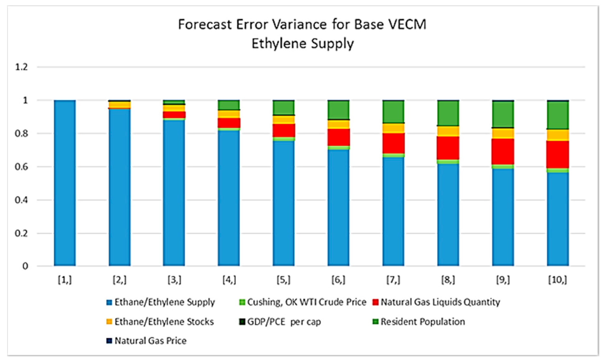
Figure 4.
Business-as-usual “base” VECM (in red) compared to nine scenarios in 2035.


Table 1.
Summary Statistics.
| Variable | Obs | Mean | Standard Deviation | Median | Trimmed Mean | Median Absolute Deviation | Minimum | Maximum | Range | Skewness | Kurtosis | Standard Error |
|---|---|---|---|---|---|---|---|---|---|---|---|---|
| Ethane/Ethylene Supply (Thousand Barrels) | 348 | 9.93 | 0.23 | 9.93 | 9.93 | 0.23 | 9.43 | 10.46 | 1.04 | 0.06 | −0.66 | 0.01 |
| Cushing, OK WTI Crude Oil Price (Dollars per Barrel) | 348 | 3.51 | 0.68 | 3.27 | 3.48 | 0.62 | 2.43 | 4.9 | 2.47 | 0.47 | −1.28 | 0.04 |
| Natural Gas Liquids Quantity (Thousand Barrels) | 348 | 10.93 | 0.16 | 10.91 | 10.91 | 0.11 | 10.64 | 11.48 | 0.85 | 1.33 | 1.92 | 0.01 |
| Ethane/Ethylene Stocks (Thousand Barrels) | 348 | 9.97 | 0.24 | 9.94 | 9.96 | 0.23 | 9.47 | 10.62 | 1.16 | 0.52 | −0.21 | 0.01 |
| GDP/PCE per Capita (in 2009 $U.S.) | 348 | 8.95 | 0.36 | 9.02 | 8.97 | 0.43 | 8.21 | 9.5 | 1.29 | −0.25 | −1.07 | 0.02 |
| Resident Population | 348 | 19.45 | 0.09 | 19.46 | 19.45 | 0.11 | 19.29 | 19.58 | 0.29 | −0.19 | −1.23 | 0 |
| Natural Gas Price (Dollars per Thousand Cubic Feet) | 348 | 1.47 | 0.4 | 1.35 | 1.44 | 0.44 | 0.96 | 2.52 | 1.56 | 0.55 | −0.91 | 0.02 |
Table 2.
Overview of Future Ethylene Supply Scenarios 2015–2050.
| SSP Scenarios | Natural Gas Feedstock Price Scenarios | ||
| SSP1 Sustainability EIA Ref. Gas Price | SSP1 Sustainability Low Gas Price | SSP1 Sustainability High Gas Price | |
| SSP3 Regional Rivalry EIA Ref. Gas Price | SSP3 Regional Rivalry Low Gas Price | SSP3 Regional Rivalry High Gas Price | |
| SSP5 Fossil-Fueled Dev. EIA Ref. Gas Price | SSP5 Fossil-Fueled Dev. Low Gas Price | SSP5 Fossil-Fueled Dev. High Gas Price | |
Table 3.
Matrix of Deterministic Coefficients for the Base VECM.
| Variables with Significance Codes | Constant |
|---|---|
| Ethane/Ethylene Supply (Thousand Barrels) | −23.6 |
| Cushing, OK WTI Crude Oil Price (Dollars per Barrel) | 5.53 |
| Natural Gas Liquids Quantity (Thousand Barrels) *** | −1.65 |
| Ethane/Ethylene Stocks (Thousand Barrels) *** | 14.00 |
| GDP/PCE per Capita (in 2009 $U.S.) * | 1.36 |
| Resident Population *** | 0.02 |
| Natural Gas Price (Dollars per Thousand Cubic Feet) | 2.50 |
| -OLS regression of the unrestricted VECM (lags 1–3) |
Significance codes: 0 ‘***’ 0.001 ‘**’ 0.01 ‘*’ 0.05 ‘.’ 0.1 ‘ ’.
Table 4.
Model Results for Future Ethylene Supply (thousand barrels per year).
| Years and % Change | “Base” VECM | SSP1 Sustainability EIA Ref. Gas Price | SSP1 Sustainability Low Gas Price | SSP1 Sustainability High Gas Price |
| 2014 (actual) | 375,309 | 375,309 | 375,309 | 375,309 |
| 2035 (projection) | 441,771 | 633,244 | 655,684 | 579,193 |
| 2050 (projection) | 481,183 | 716,908 | 752,334 | 633,876 |
| % Change from 2014–2035 | 18% | 69% | 75% | 54% |
| % Change from 2014–2050 | 28% | 91% | 100% | 69% |
| % Change from Base 2035 | 43% | 48% | 31% | |
| % Change from Base 2050 | 49% | 56% | 32% | |
| Years and % Change | “Base” VECM | SSP3 Regional Rivalry EIA Ref. Gas Price | SSP3 Regional Rivalry Low Gas Price | SSP3 Regional Rivalry High Gas Price |
| 2014 (actual) | 375,309 | 375,309 | 375,309 | 375,309 |
| 2035 (projection) | 441,771 | 435,267 | 450,691 | 398,117 |
| 2050 (projection) | 481,183 | 340,796 | 357,636 | 301,327 |
| % Change from 2014–2035 | 18% | 16% | 20% | 6% |
| % Change from 2014–2050 | 28% | −9% | −5% | −20% |
| % Change from Base 2035 | −1% | 2% | −10% | |
| % Change from Base 2050 | −29% | −26% | −37% | |
| Years and % Change | “Base” VECM | SSP5 Fossil-Fueled Dev. EIA Ref. Gas Price | SSP5 Fossil-Fueled Dev. Low Gas Price | SSP5 Fossil-Fueled Dev. High Gas Price |
| 2014 (actual) | 375,309 | 375,309 | 375,309 | 375,309 |
| 2035 (projection) | 441,771 | 830,595 | 860,029 | 759,698 |
| 2050 (projection) | 481,183 | 1,212,416 | 1,272,330 | 1,071,991 |
| % Change from 2014–2035 | 18% | 121% | 129% | 102% |
| % Change from 2014–2050 | 28% | 223% | 239% | 186% |
| % Change from Base 2035 | 88% | 95% | 72% | |
| % Change from Base 2050 | 152% | 164% | 123% |
© 2018 by the author. Licensee MDPI, Basel, Switzerland. This article is an open access article distributed under the terms and conditions of the Creative Commons Attribution (CC BY) license (http://creativecommons.org/licenses/by/4.0/).
Share and Cite
MDPI and ACS Style
Foster, G. Ethylene Supply in a Fluid Context: Implications of Shale Gas and Climate Change. Energies 2018, 11, 2967. https://doi.org/10.3390/en11112967
AMA Style
Foster G. Ethylene Supply in a Fluid Context: Implications of Shale Gas and Climate Change. Energies. 2018; 11(11):2967. https://doi.org/10.3390/en11112967
Chicago/Turabian StyleFoster, Gillian. 2018. "Ethylene Supply in a Fluid Context: Implications of Shale Gas and Climate Change" Energies 11, no. 11: 2967. https://doi.org/10.3390/en11112967
Note that from the first issue of 2016, this journal uses article numbers instead of page numbers. See further details here.