Wind Power Consumption Research Based on Green Economic Indicators


1
School of Electrical Engineering, Northeast Electric Power University, Jilin 132012, China
2
State Grid Sanmenxia Power Supply Company, Sanmenxia 472000, China
*
Author to whom correspondence should be addressed.
Energies 2018, 11(10), 2829; https://doi.org/10.3390/en11102829
Submission received: 28 September 2018
/
Revised: 18 October 2018
/
Accepted: 18 October 2018
/
Published: 19 October 2018
Abstract
:As a representative form of new energy generation, wind power has effectively alleviated environmental pollution and energy shortages. This paper constructs a green economic indicator to measure the degree of coordinated development of environmental and social benefits. To increase the amount of wind power consumption, an economic dispatch model based on the coordinated operation of cogeneration units and electric boilers was established; we also introduced the green certificate transaction cost, which effectively meets the strategic needs of China’s energy low-carbon transformation top-level system design. Wind power output has instability and volatility, so it puts higher requirements on the stable operation of thermal power units. To solve the stability problem, this paper introduces the output index of the thermal power unit and rationally plans the unit combination strategy, as well as introducing the concept of chance-constrained programming due to the uncertainty of load and wind power in the model. Uncertainty factors are transformed into load forecasting errors and wind power prediction errors for processing. Based on the normal distribution theory, the uncertainty model is transformed into a certain equivalence class model, and the improved disturbance mutated particle swarm optimization algorithm is used to solve the problem. Finally, the validity and feasibility of the proposed model are verified based on the IEEE30 node system.
1. Introduction
With the rapid development of the social economy, environmental problems and energy crises have become increasingly prominent. The green economy is an important development model for achieving sustainable development and resolving the contradiction between economic development and ecological environment [1,2]. Wind power is a new form of energy power generation. Because of the increasing installed capacity and grid-connected scale, it has significantly alleviated environmental pollution and energy crisis. Wang X et al. proposed a green certificate trading mechanism which is a supporting mechanism for the renewable energy quota system. Government and regulators allocate a certain amount of renewable energy quotas to power companies according to the situation. The quotas must be completed by delivering green certificates. The drawback is that it does not take into account the price of green certificates changes in real time with supply and demand. In this paper, based on the actual transaction data, the green certificate transaction curve is drawn, and through multiple documents, the green certificate transaction formula is formulated under the conditions of satisfying the supply and demand relationship and the government punishment mechanism [3].
The randomness and uncertainty of wind power seriously threaten the safety and economy of grid operation [4]. The error between the predicted and actual values determines the uncertainty of wind power [5]. Cong P et al. proposed a pre-active power scheduling method that considers the prediction error of renewable energy power generation to eliminate risks and reduce the cost of distribution network companies. The disadvantage is that the load prediction error is not considered [6]. Some common methods to solve problems such as randomness and uncertainty are Stochastic optimization [7], chance-constrained optimization [8], robust optimization [9], etc. These methods aid us in dealing with the uncertainty of wind power. We use the method of opportunity constraint to deal with variables. To meet the power supply and heating demand, Northeast China mainly uses coal-fired cogeneration units and thermal power units [10] for combined power generation. The region is rich in wind energy resources and has established a large number of wind farms. To increase the amount of wind power consumption, other equipment needs to be added to increase the flexibility of the system. Therefore, electric energy storage equipment [11,12] and thermal energy auxiliary equipment [13,14] have been developed and applied. The basic function of an energy storage device is to directly consume the remaining wind power. In previous papers [15,16,17], the literature validates the effectiveness of pumped storage technology in wind power consumption. Cleary Brendan et al. elaborated on the important role of compressed air storage in wind power systems and considered compressed air storage as the most attractive energy storage technology [18]. In multiple past papers [19,20,21], hydrogen storage technology not only increased the amount of wind power consumption but also saved energy. Using the remaining wind power to break down water into hydrogen and oxygen, hydrogen is stored, and hydrogen can be converted into electricity in different ways when electrical energy is needed. The basic function of the thermal energy auxiliary equipment is to use excess electric energy to generate heat, and then convert the heat into electric energy when necessary. This method reduces the output power of the cogeneration unit. This method is of great help for us to deal with the remaining problems of wind power, so an electric boiler is added in this paper to absorb wind power further. In our following study, we will further improve the research on wind power storage. Common thermal energy auxiliary equipment includes electric boilers, heat pumps and the like, etc. Chen X et al. compared the performance of electric boilers and heat storage tanks in reducing wind erosion and saving energy. The results provide a good reference for studying the comprehensive benefits of the combination of electric boilers [22]. Zidan A. et al. focused on the optimal planning of the coordinated operation between the cogeneration unit and the electric boiler in the microgrid [23]. Zhang X. et al. established an optimal scheduling model with the goal of minimizing abandonment of wind, photoelectric power, and maximizing energy storage. The optimal short-term operation of the system is studied by using the optimal algorithm of progress. The disadvantage is that the frequent planning adjustment of the unit will reduce the operating efficiency of the unit and reduce the stability of the system [24]. El-Zonkoly A. M. et al. describes a multi-objective addressing method based on particle swarm optimization and optimizes flow analysis of targets. The disadvantage is that the diversity of the population is not considered [25]. Kefayat M. et al. proposed a hybrid method based on ant colony optimization and artificial bee colony technology. The disadvantage is that there is no analysis of the computation time required by the algorithm, which is the key factor in determining the superiority of the proposed algorithm [26].
At present, in the study of economic dispatch of power systems, the mutual influence of social benefits and environmental benefits is ignored. Although the calculation of social benefits and environmental benefits alone can meet the design requirements, it is inconsistent with the actual situation, which will lead to the fact that the results obtained cannot guide the dispatch. In this paper, the green economic index is designed to coordinate the balanced development of social benefit and environmental benefit. The green economic indicator is based on the rate of reduction of pollutant emissions and the rate of economic growth. This paper constructs a mathematical model of the power system containing the wind farm and uses the method of chance constraint to deal with wind power uncertainty. The scheme is solved by the improved disturbance mutated particle swarm optimization algorithm, and the simulation is verified on the IEEE30 node test system. Finally, the feasibility of green economic indicators in economic dispatch is confirmed.
This paper is organized as follows. Section 2 establishes green economy indicators. Section 3 describes the cost of the economic scheduling model. Section 4 establishes a system optimization model. Section 5 proposes an improved perturbed variation particle swarm optimization algorithm. Section 6 analyzes the system example model based on IEEE30 nodes. Finally, Section 7 summarizes the conclusions.
2. Green Economy Index
The Green Economic Development Index uses indicators that measure the green development status of the national economy. It represents the degree of coordinated economic, environmental, and social development. Power generation strategy planning is not only to pursue social and economic benefits, but also to pursue environmental benefits unilaterally and to consider the coordinated development of the economy and the environment.
The green economy development index is implemented according to the provisions of the green development index system [27], calculated from the weighted average of the individual index of 55 indicators other than “citizen satisfaction”:
where Z is the green development index; R is number of indicators; Yr is an individual index of index r; and Wr is the weight of index Yr.
This paper mainly considers the study of the coordinated development of wind power and thermal power to maximize environmental and social benefits. In the combined operation of wind power and thermal power, environmental pollutants mainly include SO2, CO2, NO2, and soot. In thermal power plants, equipment is equipped with real-time monitoring of air pollutant emissions. When the emissions exceed the limits set by the state, it is necessary to reduce the output of thermal power units so that the pollutant emissions meet the national standards. At this time, these four indicators play an indirect role in economic dispatch. The fossil energy consumed by the operation of thermal power units is also considered in the green economy. The fossil energy is not inexhaustible, and the energy consumption also needs to meet the regulations of various power plants. At this time, the energy consumption index plays a direct role in economic dispatch. Therefore, according to the construction form of the green economy index, the environmental development index of unit GDP is proposed:
where , , , Yt,r, and Yt are the index of SO2, CO2, NO2, soot, and energy consumption, the index refers to the rate at which pollutant emissions are falling and energy consumption is falling; W1, W2, W3, W4, and W5 are weights for , , , Yt,r, and Yt.
This is an article about the economic dispatch of power systems with wind farms. The social benefit is only considered as the power generation profit, and the weight Wr takes the value 1. Therefore, the social economic benefit development index under unit GDP can be expressed as:
where Yt,GDP is GDP development index, the index refers to the growth rate of GDP.
Therefore, the green economy development index λ is designed, Z1 is the environmental development indicator under the unit GDP and Z2 is the social benefit development indicator under the unit GDP. The index λ reflects, not only environmental benefits, but also reflects social benefits. It can be seen that the green economy development coefficient is an interval indicator, it is not the ‘bigger the better’, nor ‘the smaller the better’, but should be kept within a certain range. The closer the value of λ is to 1, the better the coordination of green economy development. In this paper, through the analysis and calculation of pollutant emission data of a power plant, the green economic development index is divided into the following three sections.
When 0 < λ < 0.85, it indicates that in the process of development, certain environmental benefits have been sacrificed for the development of economic benefits;
when 0.85 < λ < 1.15, it indicates that in the process of development, environmental and economic benefits develop in harmony;
when 1.15 < λ, it indicates that in the process of development, certain economic benefits have been sacrificed for the development of environmental benefits.
3. System Scheduling Model Cost
Based on the general cost function, this paper comprehensively considers the transaction cost of the green certificate, the cost of an electric boiler, the cost of the combined heat and power unit, and the cost of wind power to establish an economic dispatching model with wind power system. The specific scheduling model is as follows.
3.1. Green Certificate Transaction Costs
We define the electric energy produced by the thermal power unit in this paper as nongreen electric energy, and the electric energy generated by the wind power unit as green electric energy. The demand for green certificates mainly comes from the Government’s mandatory quota system, forcing renewable energy consumption into energy consumption:
where Q is annual electricity demand, α(t) is quota ratio, and q(t) is the demand for green energy.
The installed capacity of renewable energy is a dynamic process [28]:
where K(t) is renewable energy installed capacity; K0 is initial capacity; i(t) is depreciation rate; d(t) is investment rate; L is average life; Ieq is partial equilibrium investment rate; Ip is a factor affecting investment profit; r is return on investment; g(t) is the amount of green energy output; and CF is the annual average power generation factor.
The interaction between supply and demand forms the price of a green certificate, and it changes in real time. Figure 1 reflects the supply and demand curve of the green certificate of thermal power plants. We set Pc(t) as the price of the green certificate:
where τ is green certificate supply and demand adjustment time and g(t) is actual power generation.
The transaction cost of the green certificate can be expressed as
where n is the number of thermal units, m is the number of wind farms, qi(t) is the green energy demand at the time t of the i-th thermal power unit, gj(t) is the green energy output at the time t of the j-th wind turbine, and ε is the green power required for the exchange unit green certificate.
3.2. Environmental Costs
The main pollutants considered in this article are SO2, NO2, and CO2. The formula for calculating environmental costs is as follows
where CS, CN, and CO are charged for SO2, NO2, and CO2 emissions, respectively.
The calculation formula for the discharge cost of various pollutants is as follows
where LS, LN, and LO are the emissions of SO2, NO2, and CO2, respectively; DS, DN, and DO are the pollution equivalence values of SO2, NO2, and CO2, respectively; JS, JN, and JO charge the cost of each pollution equivalent SO2, NO2, and CO2 emissions.
The formulas for calculating various types of pollution emissions are as follows
where Cr is the cost of coal-burning in power plants, it is mainly the fuel cost and start-stop cost of thermal power units in this paper; fS, fN, and fO are the SO2, NO2, and CO2 emissions generated by burning coal per unit of power plant consumption, respectively; J1 is the unit price of coal.
3.3. Generator Backup Cost
3.3.1. Costs of Thermal Power Units
The cost of the thermal power unit is fuel cost and start-stop cost, which are as follows
where f1 is the thermal power unit operating cost; ai, bi, and ci represent the power generation cost coefficient of thermal power unit i; Pit is the output of thermal power unit i at time t; f2 is thermal power unit start-stop cost; ui,t is the operating state of thermal power unit i during period t, ui,t = 1 indicates unit operation, ui,t = 0 indicates the unit is out of service; and Si is the starting and stopping cost of conventional unit i.
3.3.2. The Costs of the Electric Boiler and Combined Heat and Power Unit
This paper uses the extraction steam cogeneration unit. Because the cogeneration unit needs to ensure the heating demand is met and does not allow the phenomenon of downtime, only the fuel cost is considered, and the start-stop cost is not involved.
The cost of the electric boiler and combined heat and power unit is
where CCHP is the cost of combined heat and power units; CEB is the cost of electric boilers.
The relationship between the heating power and the generating power of combined heat and power units is
where PZSht is electric power under pure condensing conditions; PCHPht is an extraction turbine generating power; ChV is the thermoelectric ratio of combined heat and power unit; and HCHPht is the heating power.
Combined with the relation between the fuel cost of the conventional unit and the heat supply and power generation of the unit, the fuel cost of the unit can be obtained:
where Ai, Bi, and Ci are the coal consumption coefficients of the combined heat and power unit; M is the number of combined heat and power unit.
The total cost of the electric boiler in its service life [29,30] is
where PEBN is electric boiler capacity; uEB is unit construction cost; NEB is service life period; is maintenance ratio; νele is electric boiler operating price; WEB is electric boiler operation power consumption; and is is the social discount rate.
Due to the different operating costs corresponding to different time periods, Formula (25) is simplified in this paper and formulated as follows according to the actual situation.
where SH is the heat load per unit area; θ is the heat load factor; and T is the running time of electric boiler.
3.3.3. Rotational Standby Costs
When the wind power is connected to the grid, the on-grid electricity of the thermal power unit will be reduced and, as the scale of the wind power grid increases, the uncertainty of the grid will become more obvious. Therefore, to ensure the safe operation of the power grid, it is necessary to increase the rotating reserve capacity of the system, resulting in additional costs. The rotating standby cost of the system after the wind power is connected to the grid is
where kr is the rotational standby cost factor; klt is the percentage of prediction error of system load at time t; Plt represents the load of the system at time t; kjt is the percentage of prediction error at time t of the j-th wind turbine; and Pfjt represents the predicted output of the j-th wind turbine at time t.
3.3.4. Wind Power Costs
Wind turbines do not consume fossil energy in the process of power generation. Because the initial investment cost and operation and maintenance cost of the wind turbine is relatively high, based on the above costs, the average power generation cost of the wind turbine is approximately expressed as a linear relationship with the power generation:
where Kwjt is the cost coefficient of power generation for wind turbines in unit time t and Pjt represents the actual output of the j-th wind turbine at time t.
4. Establishment and Processing of Economic Dispatch Model
4.1. Objective Function
The objective function is set to the scheduling period T (24 h). Using the thermal power plant output indicators and green economic indicators, make the expected cost of thermal power unit, environmental cost, electric boiler cost, combined heat and power unit cost, spinning reserve capacity cost, green certificate transaction cost, and wind power cost minimum:
4.2. Restrictions
4.2.1. Power Balance Constraint of the Power Grid
The power balance constraint equation can be expressed as follows:
where PEB,t is the electric power consumed by the electric boiler to supply heat at time t and Plt is a load of the system at t time.
4.2.2. Rotating Spare Constraint
The establishment of the rotating reserve capacity is a necessary condition for the stable operation of the system. It is mainly to respond to the output fluctuations of the unit caused by load and wind power uncertainty. This paper establishes positive and negative rotation reserve capacity constraints based on chance-constrained programming, and deals with the uncertainty of load and wind turbine output prediction value:
Positive rotation reserve capacity constraint:
Negative rotation reserve capacity constraint:
where Pi,max and Pi,min are the maximum and minimum output of the i-th thermal power unit, respectively; and are the maximum and minimum output of the h-th cogeneration unit, respectively; Pit,max and Pit,min are the maximum and minimum output of the i-th thermal power unit at time t, respectively; and are the maximum and minimum output of the h-th cogeneration unit at time t, respectively; rui and rdi are the upward climbing rate and downward climbing rate of the i-th thermal power unit, respectively; ruh and rdh are the upward climbing rate and downward climbing rate of the h-th cogeneration unit, respectively; Klu is the system load positive fluctuation coefficient; Kwu and Kwd are positive and negative rotation reserve factors for wind farms; and β1 and β2 are confidence levels.
4.2.3. Thermal Power Unit Output Stability Index Constraint
In the process of wind power grid connection, the stability of the unit’s planned output has a great impact on the unit’s operating efficiency. Frequent planning adjustment will greatly reduce the unit’s operating efficiency. For this reason, the unit’s planned output index is introduced in this paper to plan the unit combination strategy rationally. To strive to maximize unit efficiency [31].
where ηmin is the minimum value of planned output stability; is the limit of stability average; is limit of the minimum value of stability; Δ is full-day maximum absolute climbing rate; Pi,t+1 and Pi,t are the outputs of the thermal power plant i in t + 1 period and t period, respectively; and NT is number of scheduled time slots.
The stability index of all generator sets output curves of the system is the arithmetic mean of the indicators of all generator sets:
4.2.4. Output Constraint and Climbing Rate Constraint of Conventional Units and Combined Heat and Power Units
The output constraint and climbing rate constraint formula can be expressed as follows:
where Pi,max and Pi,min are the maximum and minimum output of the i-th thermal power unit, respectively; and are the maximum and minimum output of the h-th combined heat and power unit, respectively.
The unit’s maximum up-down output adjustment range in unit time is called climbing rate, that is
Most articles on economic dispatch consider start-stop constraints, and this paper also considers start-stop constraints. This is not described here, but is detailed in the literature [3].
4.3. Opportunistic Constraint Transformation
The uncertainty of wind power brings a series of problems to the system. In this paper, the wind power forecast value is taken as the sum of the actual wind power dispatching power and the wind power forecasting error, and the load is treated the same:
where ξklt is the load prediction error value of the system at time t, which can be obtained by klt; ξkjt is the power prediction error value of the j-th wind farm at time t, which can be obtained by kjt; both errors are subject to a normal distribution with a mean of 0.
The standard deviations of wind power and load forecasting errors are
where σjt is the standard deviation of the power prediction error at time t of the j-th wind farm; PjN is the installed capacity of the j-th wind farm; and σlt is the standard deviation of the load prediction error at time t.
This paper uses the equivalence class to deal with the constraint conditions. The form of the opportunity constraint is
Assuming that the form of g(X,ξ) can be expressed as h(X)-ξ, the above equation can be expressed as
where h(X) is a function of decision vector X; ξ is a random variable, and the probability distribution function is φ(·).
For each given confidence level α (0 ≤ α ≤ 1), there is one or more Kα:
If a smaller number is used instead of Kα, the probability of the left end will become larger, so is established only if h(X) ≤ Kα. An equivalent form of is
When solving Kα, it is found that is always established, and it is obtained by .
where φ−1 is the inverse function of φ, the solution of may not be unique, equivalently, the function φ−1 is multivalued, for which we choose the largest one:
Based on the above-described opportunity constraint processing method, it is assumed that the wind power prediction error value and the load prediction error values are independent of each other; the positive rotation reserve capacity constraint can be expressed as
where is the inverse function of φ1, φ1 is the probability distribution function of , and the random variable Z1 obeys a normal distribution:
The equivalent determination model for the same negative rotation reserve capacity is
where is the inverse function of φ2, φ2 is the probability distribution function of , and the random variable Z2 obeys a normal distribution:
5. Improved Particle Swarm Optimization Algorithm for Disturbance Variation
5.1. Improved Particle Swarm Optimization
The standard particle swarm optimization algorithm is composed of two core algorithms of particle velocity and position update equation, respectively:
where ω is inertia weight; i denotes the i-th particle; j represents the j dimension; vij(t) indicates the j-th flight velocity component of particle i when it evolved to t generation; xij(t) represents the j-th position component of particle i when it evolved to t generation; pbestij(t) represents the j-dimensional individual optimal position pbest component of particle i when it evolved to t generation; gbestj(t) represents the j-th component of the best position gbest of the entire particle swarm evolution to t; C1 and C2 are learning factors; and r1 and r2 are [0,1] random numbers.
The perturbation variable particle swarm optimization algorithm is a combination of a genetic algorithm and Gaussian white noise. The global convergence of the algorithm is guaranteed while the population diversity is improved.
In this algorithm, for each particle x = (x1,x2…xn) with mutation probability Pm, where Pm is determined by the complexity and experience of the optimization function. Generally, the value can be between 0.05 and 0.15. The mutant particle is
where xi,j is the coordinate of the particle in the j-th dimension; gbesti,j is the coordinate of the global optimal value in the j dimension; and σ is Gaussian white noise random number, set the noise level to 0 dBW.
In the standard particle swarm optimization (PSO) algorithm, the usual approach is to place the particle on the boundary when a particle flies out of the feasible region during the search. The disadvantage of standard PSO is that it is easy to trap the particle into the local optimum if there is a local optimum near the boundary, thus causing stagnation. This also causes multiple particles to aggregate toward multiple boundaries in multiple dimensions. After several iterations, the behavior of particles concentrated at the boundary will inevitably tend to be the same, to reduce the diversity of the entire population of particles. In the improved algorithm, the particles beyond the boundary are mutated in the following way.
where and are the lower and upper bounds of the j-th dimension of the particle. This is equivalent to reproducing particles in the domain beyond the boundary.
To better overcome the algorithm into local search, it is possible to determine the change of inertia weight according to the degree of premature convergence and the individual fitness value based on improved algorithms. Set the fitness value of particle i is fi; the optimal particle adaptation value is fm; the average fitness value of the particle swarm is ; we then average the fitness value better than favg to get ; define . Then, classify groups into three subgroups based on fi, favg and , perform different adaptive operations separately. That is:
The first type of particle is a better particle, which is close to the optimal global solution, give a smaller inertia weight to strengthen local search capabilities; the second type of particle is the general one which has good global and local search capabilities, we do not need to change its inertia weight; the third type of particle is the inferior one, adapting the parameters of the adaptive adjustment genetic algorithm to adjust the parameters. k1 and k2 are control parameters, use k1 to control the upper limit of ω; k2 is mainly used to control the regulation ability of the formula. When the algorithm stops, if the particle distribution is more dispersed, then Δ is larger, we then need to reduce ω to make particles have stronger local search ability; if the particle distribution is more concentrated, then Δ is smaller, and we need to increase ω to make particles have strong global search ability.
5.2. Algorithm Flow Chart
The improved algorithm flow chart is shown in Figure 2.
6. Analysis of Examples
6.1. Study Parameters
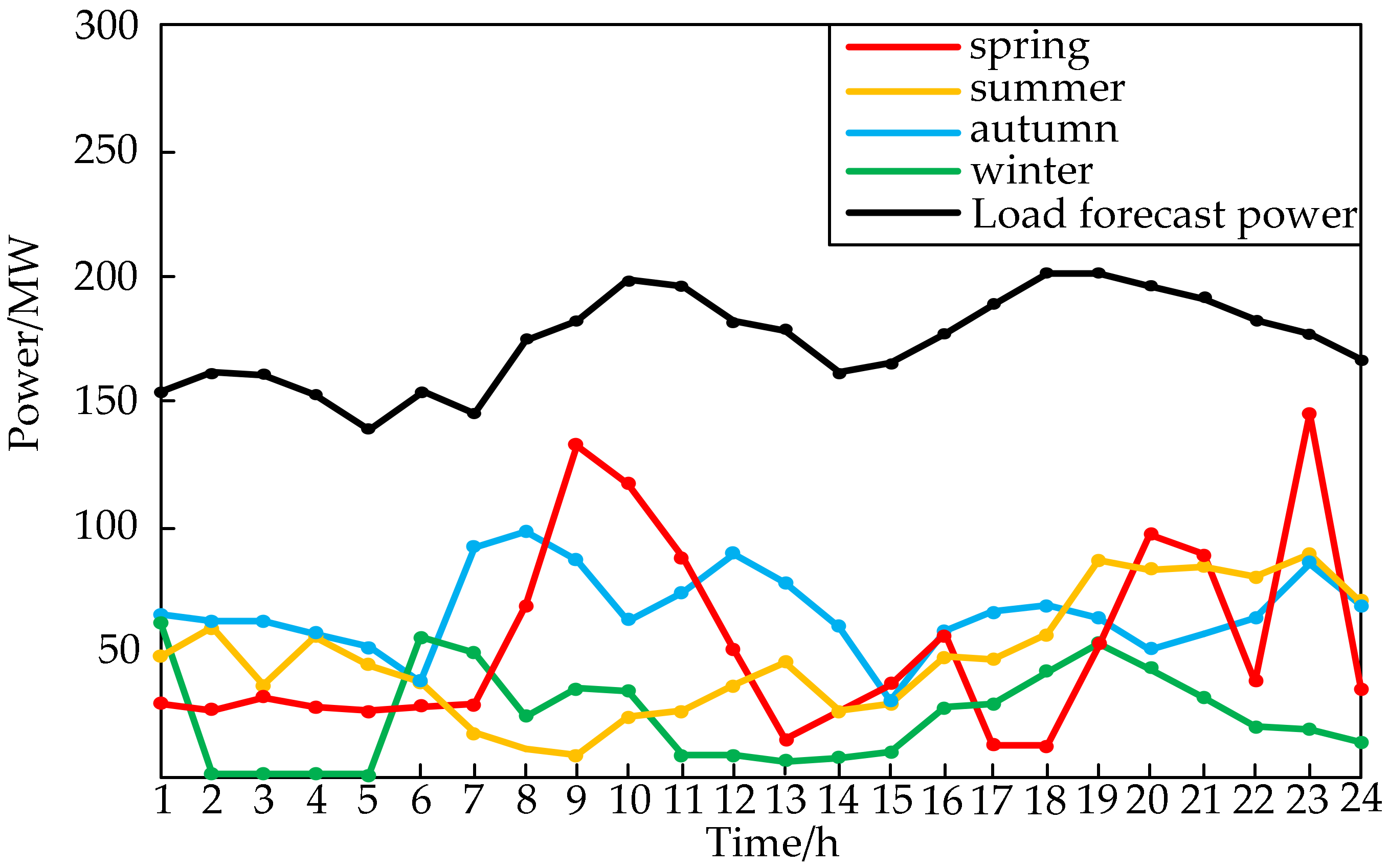
This paper uses the IEEE30 node standard test system for power systems. The example system is shown in Figure 3. The cogeneration unit replaces the 1st and 2nd units in the original system, respectively; the wind farm grid connection node is 16. The relevant parameters of the thermal power unit are shown in Table 1, and the cogeneration unit is shown in Table 2. In this paper, the wind power consumption is studied according to the wind power field data measured in a certain area. In order to increase the universality of the scheduling process, this paper selects four representative days of spring, summer, autumn, and winter in a year for analysis, the characteristics of four seasons are shown in Table 3. The scheduling day is divided into 24 scheduling periods for research. Curve of actual measurement of wind power output and predictive power of load are as shown in Figure 4. The parameter settings in the optimization scheduling process are as follows, DS, DN, and DO are 0.95 kg, 0.95 kg, and 16.7 kg, respectively; JS, JN, and JO are $0.0893, $0.0893, $0.0893, respectively; fS, fN, and fO are 8.5 kg, 7.4 kg, and 16.7 kg, respectively; J1 is 74.448 $/t; the rotational spare cost coefficient kr is 34.39 $/MW; the load prediction error kl is 5%; and the forecast error kjw of wind farm i is 15%.
To compare the effects on wind power consumption after the addition of electric boilers, cogeneration units, and green certificate transaction costs, the examples are simulated in the following three ways, as shown in Table 4.
6.2. Comparative Analysis of Different Scheduling Modes
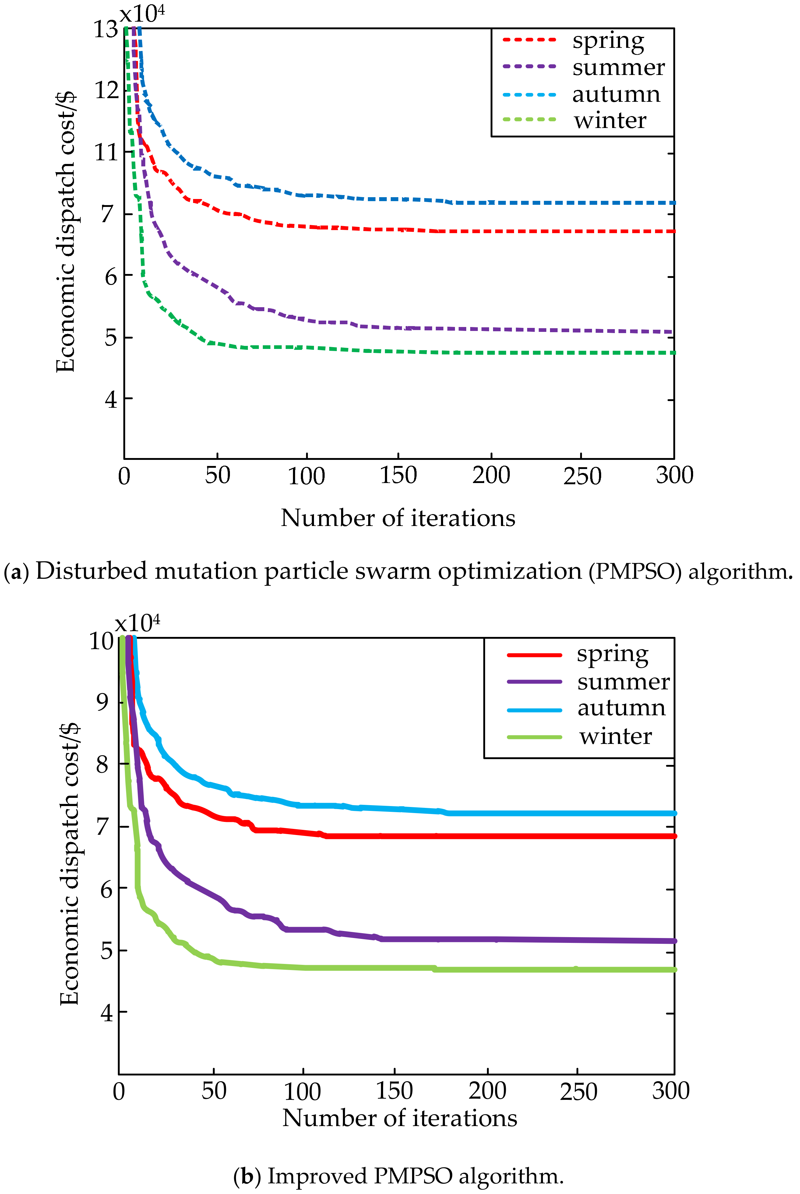
We used the disturbed mutation particle swarm optimization (PMPSO) and the improved perturbed variation particle swarm optimization to solve models, which consider wind power systems with four important periods of the year, for the following analysis. In the process of solving the four dispatch days, the load is kept unchanged, and the change curve of the system comprehensive cost is shown in Figure 5.
It can be seen from Table 5 that the improved PMPSO algorithm improves the optimization speed and also improves the optimization precision.
As can be seen from Figure 5, within the four typical scheduling days selected economic costs are monotonically decreasing and eventually converge to a minimum; this shows the reliability of the results obtained. Therefore, the comprehensive operation cost can be significantly reduced through reasonable scheduling of thermal power units, electric boilers, cogeneration unit, and wind power. It can also improve the consumption of wind power and the economy of grid-connected operation.
The value range of the green economy index is simply divided into three segments, which are 0 < λ < 0.85, 0.85 < λ < 1.15, and 1.15 < λ; the scheduling analysis is performed for each index interval by mode 1. The results are visible in Table 6. When 0.85 < λ < 1.15, it is considered that the environmental and social benefits are coordinated; the minimum comprehensive cost is the most suitable range of economic dispatch value. In contrast, when 0 < λ < 0.85, sacrificing part of the environmental benefits, pursuing greater social and economic benefits, wind power consumption decreased by 8.95% on average, and overall cost increased by an average of 4.8125 K$, the coal consumption cost of the thermal power unit and cogeneration unit increases. The green certificate produced by wind power does not meet the government-defined quota, and additional certificates are required to complete the task, increasing the cost of green certificate transactions. When 1.15 < λ, some social benefits are sacrificed in order to seek greater environmental benefits, and wind power consumption increased by 5.5175% on average and overall cost increased by an average of 6.9325 K$, the coal consumption cost of thermal power units and cogeneration units is reduced. Although the amount of wind power consumption is increased, the large number of wind power grids makes the system require more spare capacity to cope with wind power uncertainty and randomness. Considering that the green economy index affects the results of the economic dispatch model, when the value range is 0.85 < λ < 1.15, the economic dispatch model can find the optimal solution.
This paper makes a comparison between increasing the output constraint and not increasing the output constraint and it can be seen from Figure 6 that the stability index of the generator set without increasing the output constraint is 63%, and after the output force constraint is increased, the stability index of the generator set is 75%. It can be obtained that the stability of the unit is greatly improved after increasing the output constraint of the unit. For power generation cost, after increasing the output constraint, coal consumption increased by 0.45%, and coal consumption value increased. However, the coal consumption function in the optimization model shows a static curve of the coal consumption of the generating set, which does not satisfy the dynamic adjustment process under the frequent fluctuation of the power output of the generating set. The actual coal consumption will increase greatly when the power generation unit frequently adjusts its output, resulting in frequent changes in operating conditions. According to the actual operation data of a power plant unit, it can be roughly estimated that the output fluctuation of 1 MW will increase the dynamic coal consumption by 0.02 t. Therefore, the coal consumption after the increase in the output of the thermal power unit should be low, and the output force does not increase the actual coal consumption. It can be seen that considering the power generation stability of the thermal power unit can effectively improve the operating efficiency of the unit.
Figure 7 shows the simulation of a system for the whole year. The stability of the thermal power unit is 83%, and the stability is improved by nearly 19%. It can be concluded that increasing the output constraints of thermal power units has significant economic benefits for actual production. Therefore, in this example, the output of the thermal power unit is increased.
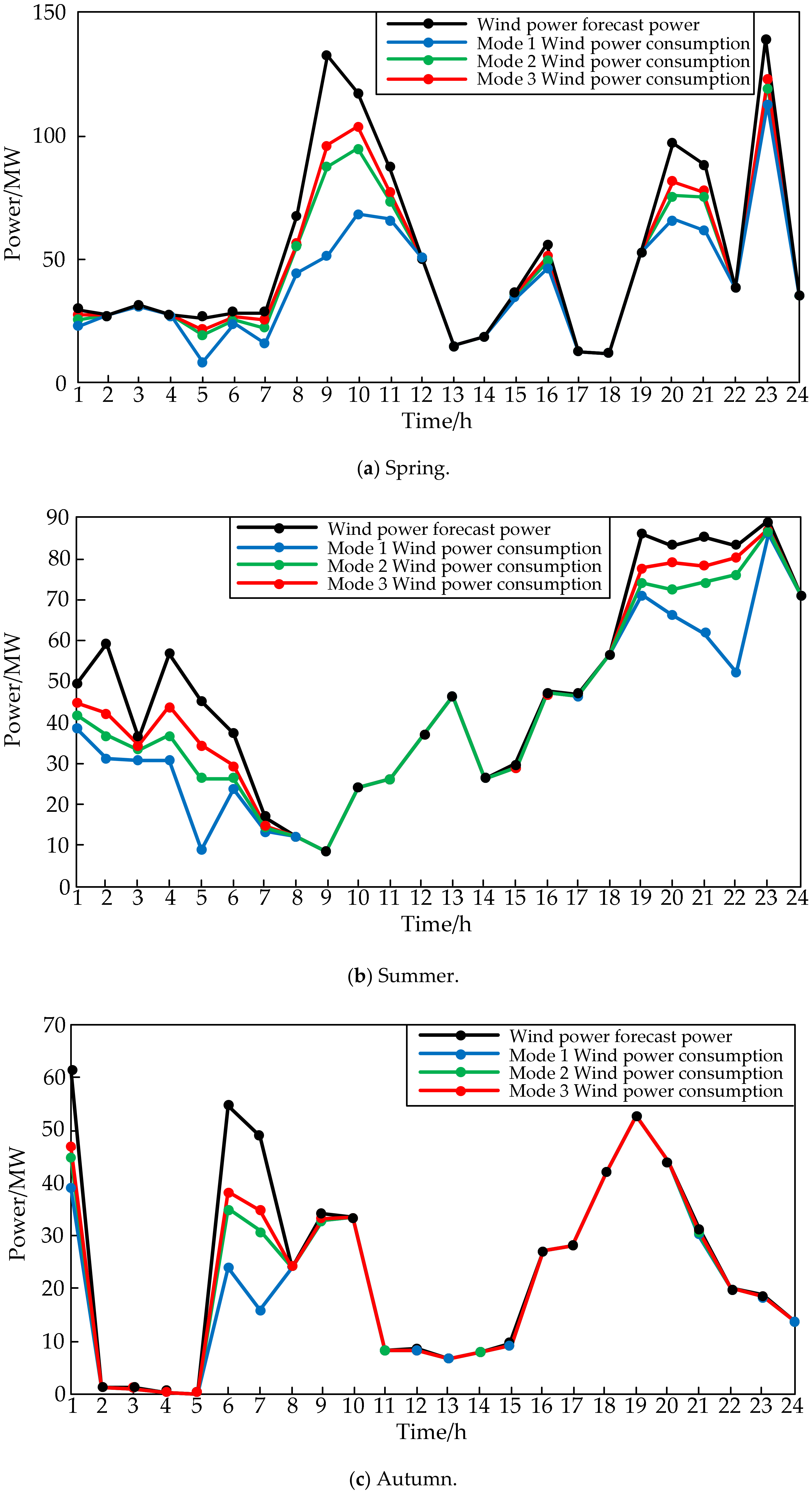
When the overall operating cost is the lowest, the amount of wind power consumption is shown in Figure 8; the start-stop results of thermal power units are shown in Table 7; the start-stop period of thermal power units is shown in Table 8.
As can be seen from Figure 8, wind power output exhibits a certain degree of randomness and volatility, and at the same time presents a certain degree of antipeaking. The wind power within the four dispatch days has a certain amount of wind abandon power that mainly occurs in the early morning and late night hours. At this stage, wind power output is larger, but the load demand is lower. To ensure the balance of power supply and demand in the operation of the power grid, a certain wind abandonment phenomenon occurs.
From Table 7, it can be seen that the shutdown of the thermal power unit during operation has occurred, and the number of starts and stops is within the maximum number of unit limits, which ensures the normal operation of the unit. Table 8 shows the time when the unit starts and stops, it can be seen that the start and stop of the unit mainly occur from 0:00 to 5:00. At this time, the load is at a low level, but the wind power output is higher. To increase the power of wind power, shutting down the unit with operational constraints allowed to reduce the output of thermal power units.
To verify the superiority of the transaction cost of the green certificate, the cost of the electric boiler, and the cogeneration unit in this paper, it is compared with the traditional dispatch method. When the green economic indicator is 0.85 < λ < 1.15, the comparison results are shown in Table 9 and Table 10.
It can be seen from Table 9 that under different scheduling modes, the pollutant emission will decrease first and then change with the increase of wind power on-grid. It indicates that the grid-connected consumption of wind power can reduce the output of thermal power units, thereby reducing pollutant emissions. However, when the capacity of the wind farm increases to the limit of consumption, the amount of wind power consumption remains unchanged, and the amount of pollutants discharged remains unchanged. In the same situation of wind power on-grid, Model 1 emits less pollutants than the other two scheduling models, which is more beneficial to the environment.
As can be seen from Table 10, model 1 has the lowest overall cost in terms of overall cost. Regarding overall costs, after the electric boiler and the cogeneration unit are added to model 1, the wind power is further absorbed, the cost of thermal power is reduced, and the cost of wind power is increased. Under the influence of the green certificate trade, the increase of green economy indicators has played an important role in balancing the green economy and social economy. Although the start-up and shutdown of the thermal power unit in model 1 caused a start-stop cost, it can significantly reduce the output of the thermal power unit, reduce the environmental cost caused by the thermal power unit, increase the amount of wind power consumption, and reduce the cost of the green certificate.
6.3. The Influence of Index Weight on Scheduling Results
The green economic indicators established in this paper mainly contain two kinds of quantities, one is the change of pollutant discharge rate, and the other is the weight value of pollutant parameters. The setting of the parameter weight value has a great influence on the scheduling result. The parameter weight values used in the scheduling model of this paper are shown in Table 11. The weight value of each pollutant is separately adjusted by 5% and 10%, and the overall cost is obtained by the operation of mode 1, as shown in Table 12.
It can be seen from Table 12, the cost of the scheduling model fluctuates when the weight value is adjusted by 5%, but the change is not obvious. When the weight value is adjusted by 10%, a significant change in cost is caused. The main source of pollutants is the burning of fossil fuels. When the weights of pollutant parameters and energy parameters change, the output of the thermal power unit will change, and in order to meet the load requirements, the wind power on-grid needs to be increased. In order to cope with the impact of wind power uncertainty, it is necessary to increase the corresponding rotating reserve capacity. The change of weight also caused the start and stop of some thermal power units, resulting in the start and stop costs of the unit. To sum up, the weight of the pollutant parameters cannot be arbitrarily changed, and the scheduling cost is greatly increased due to unreasonable changes. According to the calculation of the cost change under each parameter, if necessary, the weight can be adjusted within 5%.
7. Conclusions
This paper takes the lowest comprehensive operating cost as the goal, fully considers the fuel cost, start-stop cost, environmental cost, rotating standby cost, green certificate cost, electric boiler, and cogeneration cost of the thermal power unit, and establishes consideration of green economic indicators and the unit output. The indicator’s economic dispatch model with wind farms is solved by the improved perturbed variation particle swarm optimization algorithm for disturbance variation for the IEEE30 node example system. The following conclusions can be drawn. (1) After the addition of green economic indicators, the current scheduling plan is closer to reality than the conventional economic dispatch plan, and has a guiding role in the adjustment of the unit. (2) Compared with the literature [8], the same is used for the opportunistic constraint method, but this paper decomposes the uncertainty of wind power and load into two parts: actual value and prediction error value. This a more targeted approach, reducing the difficulty of solving while describing the model. (3) Compared with the literature [24], this paper adds the stability constraint of the unit output, which restricts the frequent adjustment of the thermal power unit plan and improves the system operation stability. (4) Compared with the literature [25,26], the improved perturbed variation particle swarm optimization algorithm applied in this paper has fewer iterations, and the solution accuracy is slightly improved. In the solution process, the population diversity problem is fully considered, and the solution obtained is more convincing.
With the deepening of research on wind power consumption based on green economic indicators, we found that there is still a lot of work to be done.
First, the green economy indicators need to be further improved, and more influencing factors will be added to the new green economic indicators after being verified and calculated. Due to the difficulty of data collection, we spend a lot of time researching.
Secondly, to improve the environmental cost formula and introduce the calculation idea of LCCA (Life Cycle Cost Analysis), taking into account not only the initial cost of calculating the cost, but also all the costs incurred in later operation: maintenance and repair and final disposal.
In the end, the involvement of other clean energy sources will also have an impact on joint operations and have greater research space.
Author Contributions
X.W. and Y.Z. conceived the theory and built the model; J.W., Y.C., and J.T. performed the experiments and analyzed the data; X.W. and Y.Z. wrote the paper.
Funding
This research is funded by the National Natural Science Foundation of China under grant number 51777027.
Conflicts of Interest
The authors declare no conflicts of interest.
References
- Stosic Mihajlovic, L.; Trajkovic, S. Modern economy: Features and developments. J. Process Manag. 2016, 4, 17–25. [Google Scholar] [CrossRef]
- Loiseau, E.; Saikku, L.; Antikainen, R.; Droste, N.; Hansjürgens, B.; Pitkänen, K.; Leskinen, P.; Kuikman, P.; Thomsen, M. Green economy and related concepts: An overview. J. Clean. Prod. 2016, 139, 361–371. [Google Scholar] [CrossRef]
- Wang, X.; Wang, J.; Tian, B.; Cui, Y.; Zhao, Y. Economic Dispatch of the Low-Carbon Green Certificate with Wind Farms Based on Fuzzy Chance Constraints. Energies 2018, 11, 943. [Google Scholar] [CrossRef]
- Lowery, C.; O’Malley, M. Impact of Wind Forecast Error Statistics Upon Unit Commitment. IEEE Trans. Sustain. Energy 2012, 3, 760–768. [Google Scholar] [CrossRef] [Green Version]
- Luickx, P.J.; Delarue, E.D.; D’Haeseleer, W.D. Impact of large amounts of wind power on the operation of an electricity generation system: Belgian case study. Renew. Sustain. Energy Rev. 2010, 14, 2019–2028. [Google Scholar] [CrossRef]
- Cong, P.; Tang, W.; Zhang, L.; Zhang, B.; Cai, Y. Day-Ahead Active Power Scheduling in Active Distribution Network Considering Renewable Energy Generation Forecast Errors. Energies 2017, 10, 1291. [Google Scholar] [CrossRef]
- Constantinescu, E.M.; Zavala, V.M.; Rocklin, M.; Lee, S.; Anitescu, M. A Computational Framework for Uncertainty Quantification and Stochastic Optimization in Unit Commitment with Wind Power Generation. IEEE Trans. Power Syst. 2011, 26, 431–441. [Google Scholar] [CrossRef]
- Wang, Q.; Guan, Y.; Wang, J. A Chance-Constrained Two-Stage Stochastic Program for Unit Commitment with Uncertain Wind Power Output. IEEE Trans. Power Syst. 2012, 27, 206–215. [Google Scholar] [CrossRef]
- Lorca, Á.; Sun, X.A. Adaptive Robust Optimization With Dynamic Uncertainty Sets for Multi-Period Economic Dispatch Under Significant Wind. IEEE Trans. Power Syst. 2015, 30, 1702–1713. [Google Scholar] [CrossRef]
- Li, Z.; Wu, W.; Shahidehpour, M.; Wang, J.; Zhang, B. Combined Heat and Power Dispatch Considering Pipeline Energy Storage of District Heating Network. IEEE Trans. Sustain. Energy 2015, 7, 12–22. [Google Scholar]
- Yao, E.; Wang, H.; Liu, L.; Xi, G. A Novel Constant-Pressure Pumped Hydro Combined with Compressed Air Energy Storage System. Energies 2014, 8, 154–171. [Google Scholar] [CrossRef] [Green Version]
- Xiong, M.; Gao, F.; Liu, K.; Chen, S.; Dong, J. Optimal Real-Time Scheduling for Hybrid Energy Storage Systems and Wind Farms Based on Model Predictive Control. Energies 2015, 8, 8020–8051. [Google Scholar] [CrossRef] [Green Version]
- Long, H.; Xu, R.; He, J. Incorporating the Variability of Wind Power with Electric Heat Pumps. Energies 2011, 4, 1748–1762. [Google Scholar] [CrossRef] [Green Version]
- Rong, S.; Li, W.; Li, Z.; Sun, Y.; Zheng, T. Optimal Allocation of Thermal-Electric Decoupling Systems Based on the National Economy by an Improved Conjugate Gradient Method. Energies 2016, 9, 17. [Google Scholar] [CrossRef]
- Hozouri, M.A.; Abbaspour, A.; Fotuhi-Firuzabad, M.; Moeini-Aghtaie, M. On the Use of Pumped Storage for Wind Energy Maximization in Transmission-Constrained Power Systems. IEEE Trans. Power Syst. 2015, 30, 1017–1025. [Google Scholar] [CrossRef]
- Helseth, A.; Gjelsvik, A.; Mo, B.; Linnet, Ú. A model for optimal scheduling of hydro thermal systems including pumped-storage and wind power. IET Gener. Transm. Distrib. 2013, 7, 1426–1434. [Google Scholar] [CrossRef]
- Sousa, J.A.M.; Teixeira, F.; Faias, S. Impact of a price-maker pumped storage hydro unit on the integration of wind energy in power systems. Energy 2014, 69, 3–11. [Google Scholar] [CrossRef]
- Cleary, B.; Duffy, A.; Oconnor, A.; Conlon, M.; Fthenakis, V. Assessing the Economic Benefits of Compressed Air Energy Storage for Mitigating Wind Curtailment. IEEE Trans. Sustain. Energy 2015, 6, 1021–1028. [Google Scholar] [CrossRef]
- Yuan, R.; Ye, J.; Lei, J.; Li, T. Integrated Combined Heat and Power System Dispatch Considering Electrical and Thermal Energy Storage. Energies 2016, 9, 474. [Google Scholar] [CrossRef]
- Melo, D.F.R.; Chang-Chien, L.-R. Synergistic Control between Hydrogen Storage System and Offshore Wind Farm for Grid Operation. IEEE Trans. Sustain. Energy 2013, 5, 18–27. [Google Scholar] [CrossRef]
- Trifkovic, M.; Sheikhzadeh, M.; Nigim, K.; Daoutidis, P. Modeling and Control of a Renewable Hybrid Energy System with Hydrogen Storage. IEEE Trans. Control Syst. Technol. 2013, 22, 169–179. [Google Scholar] [CrossRef]
- Chen, X.; Kang, C.; O’Malley, M.; Xia, Q.; Bai, J.; Liu, C.; Sun, R.; Wang, W.; Li, H. Increasing the Flexibility of Combined Heat and Power for Wind Power Integration in China: Modeling and Implications. IEEE Trans. Power Syst. 2015, 30, 1848–1857. [Google Scholar] [CrossRef]
- Zidan, A.; Gabbar, H.A. DG Mix and Energy Storage Units for Optimal Planning of Self-Sufficient Micro Energy Grids. Energies 2016, 9, 616. [Google Scholar] [CrossRef]
- Zhang, X.; Ma, G.; Huang, W.; Chen, S.; Zhang, S. Short-Term Optimal Operation of a Wind-PV-Hydro Complementary Installation: Yalong River, Sichuan Province, China. Energies 2018, 11, 868. [Google Scholar] [CrossRef]
- El-Zonkoly, A.M. Optimal placement of multi-distributed generation units including different load models using particle swarm optimisation. Swarm Evolut. Comput. 2011, 5, 760–771. [Google Scholar] [CrossRef]
- Kefayat, M.; Ara, A.L.; Niaki, S.A.N. A hybrid of ant colony optimization and artificial bee colony algorithm for probabilistic optimal placement and sizing of distributed energy resources. Energy Convers. Manag. 2015, 92, 149–161. [Google Scholar] [CrossRef]
- National Development and Reform Commission. The Provisions of the Green Development Index System. Available online: http://www.ndrc.gov.cn/fzgggz/hjbh/hjjsjyxsh/201612/t20161222_832315.html (accessed on 12 December 2016).
- Fang, F. Operation Planning and Evaluation on the Benefit of Joint Operation between Wind Power and Thermal Power Based on the Green Economy. Master’s Thesis, North China Electric Power University, Beijing, China, 29 March 2013. [Google Scholar]
- Lyu, Q.; Jiang, H.; Chen, T. Wind Power Accommodation by Combined Heat and Power Plant with Electric Boiler and Its National Economic Evaluation. Autom. Electr. Power Syst. 2014, 38, 6–12. [Google Scholar]
- Jiang, H. Research on Accommodation Curtailed Wind Power by CHP Installed Electric Boilers. Master’s Thesis, Dalian University of Technology, Dalian, China, 4 May 2013. [Google Scholar]
- Cai, Q.; Yang, Y. The day-ahead scheduling plan model and method considering the output stability. Eng. Des. 2018, 46–49. [Google Scholar]
Figure 1.
Supply and demand curve of the green certificate exchange market.

Figure 2.
Algorithm flowchart.

Figure 3.
IEEE30 node test system diagram.

Figure 4.
The curve of wind power output and predicted power of the load.

Figure 5.
Comprehensive operating cost curve.

Figure 6.
Thermal power unit output curve.

Figure 7.
The stability of the output curve of a system thermal power unit.

Figure 8.
Wind power forecasting power and consumption power.


Table 1.
Conventional unit parameters.
| Unit | Pmax/MW | Pmin/MW | rui/(MW/h) | rdi/(MW/h) | /h | /h | Si/($/t) | Vi,max/t | Fuel Cost Factor | ||
|---|---|---|---|---|---|---|---|---|---|---|---|
| ai/($·MW−2·h−1) | bi/($·MW−1·h−1) | ci/($·h−1) | |||||||||
| 3 | 50 | 25 | 25 | 25 | 2 | 2 | 26.8 | 2 | 0.0109 | 12.89 | 6.78 |
| 4 | 35 | 15 | 17.5 | 17.5 | 1 | 1 | 23.82 | 2 | 0.0697 | 26.24 | 31.66 |
| 5 | 30 | 12 | 15 | 15 | 1 | 1 | 22.33 | 2 | 0.0283 | 37.69 | 17.95 |
| 6 | 40 | 15 | 20 | 20 | 2 | 2 | 23.82 | 2 | 0.0128 | 17.82 | 10.15 |
Table 2.
Parameters of CHP unit.
| Unit | /MW | /MW | /MW | Ai/[$·MW−2·h−1] | Bi/[$·(MW·h)−1] | Ci/($·h−1) | cv | cm | ruh/(MW/h) | rdh/(MW/h) |
|---|---|---|---|---|---|---|---|---|---|---|
| 1 | 200 | 100 | 250 | 0.00066 | 1.97883 | 5.80694 | 0.15 | 0.75 | 50 | 50 |
| 2 | 200 | 100 | 250 | 0.00066 | 1.97883 | 5.80694 | 0.15 | 0.75 | 50 | 50 |
Table 3.
Characteristics of the four seasons.
| Project | Precipitation/mm | Seasonal Mean Temperature/°C | Atmospheric Pressure/hPa | Wind Velocity (Different Heights) | ||||
|---|---|---|---|---|---|---|---|---|
| Season | 10 m | 40 m | 60 m | 80 m | ||||
| Spring | 40–140 | 6.4 | 994.5 | 5.20 | 6.53 | 7.37 | 7.77 | |
| Summer | 270–570 | 21.0 | 988.3 | 3.37 | 4.10 | 5.13 | 5.37 | |
| Autumn | 45–165 | 5.9 | 999.97 | 4.10 | 5.70 | 6.67 | 7.17 | |
| Winter | 2–42 | −13.5 | 1005.8 | 3.80 | 5.40 | 6.20 | 6.70 | |
Table 4.
Unit combination method.
| Project | Thermal Power Unit | Wind Turbines | Electric Boiler | Cogeneration Unit | Green Credentials | |
|---|---|---|---|---|---|---|
| Mode | ||||||
| Mode 1 | √ | √ | √ | √ | √ | |
| Mode 2 | √ | √ | √ | √ | ||
| Mode 3 | √ | √ | ||||
Table 5.
Comparison between PMPSO algorithm and improved PMPSO algorithm.
| Project | Number of Iterations/Times | Economic Dispatch Cost/k$ | |||
|---|---|---|---|---|---|
| Period | PMPSO | Improved PMPSO | PMPSO | Improved PMPSO | |
| Spring | 157 | 114 | 68.46 | 68.22 | |
| Summer | 171 | 142 | 52.62 | 52.54 | |
| Autumn | 221 | 182 | 73.59 | 73.36 | |
| Winter | 136 | 107 | 47.53 | 47.32 | |
Table 6.
Comprehensive cost and wind power consumption under each interval of green economic indicators.
Table 6.
Comprehensive cost and wind power consumption under each interval of green economic indicators.
| Project | Economic Dispatch Cost/k$ | Wind Power Consumption/% | |||||||
|---|---|---|---|---|---|---|---|---|---|
| Range | Spring | Summer | Autumn | Winter | Spring | Summer | Autumn | Winter | |
| 0 < λ < 0.85 | 72.93 | 57.36 | 78.32 | 52.08 | 72.13 | 76.82 | 69.87 | 78.55 | |
| 0.85 < λ < 1.15 | 68.22 | 52.54 | 73.36 | 47.32 | 81.09 | 85.76 | 78.92 | 87.41 | |
| 1.15 < λ | 74.83 | 59.62 | 80.55 | 54.17 | 87.37 | 91.29 | 84.17 | 93.22 | |
Table 7.
Unit commitment results.
| Unit | Number of Starts and Stops/Time | |||
|---|---|---|---|---|
| Spring | Summer | Autumn | Winter | |
| Unit 3 | 1 | 1 | 1 | 1 |
| Unit 4 | 2 | 1 | 1 | 1 |
| Unit 5 | 1 | 1 | 1 | 1 |
| Unit 6 | 1 | 1 | 1 | 1 |
Table 8.
Unit start and stop period.
| Time | Number of Starts and Stops/Time | |||
|---|---|---|---|---|
| 0:00–5:00 | 6:00–11:00 | 12:00–17:00 | 18:00–23:00 | |
| Spring | 4 | 0 | 0 | 1 |
| Summer | 4 | 0 | 0 | 0 |
| Autumn | 4 | 0 | 0 | 0 |
| Winter | 4 | 0 | 0 | 0 |
Table 9.
Comparison of pollutant emissions under different scheduling models.
| Emissions/t | Mode 1 | Mode 2 | Mode 3 | |||||||
|---|---|---|---|---|---|---|---|---|---|---|
| Electricity/MW | SO2 | CO2 | NO2 | SO2 | CO2 | NO2 | SO2 | CO2 | NO2 | |
| 0 | 1.172 | 2.344 | 0.993 | 4.838 | 9.673 | 3.967 | 7.861 | 15.717 | 6.297 | |
| 10 | 1.168 | 2.331 | 0.896 | 4.826 | 9.651 | 3.958 | 7.194 | 14.378 | 6.173 | |
| 20 | 1.163 | 2.328 | 0.913 | 4.774 | 9.547 | 3.877 | 6.937 | 13.884 | 6.021 | |
| 30 | 0.997 | 1.991 | 0.904 | 4.782 | 9.562 | 3.862 | 6.928 | 13.856 | 5.892 | |
| 40 | 0.985 | 1.975 | 0.879 | 4.621 | 9.232 | 3.729 | 6.834 | 13.697 | 5.773 | |
| 50 | 0.972 | 1.943 | 0.871 | 4.597 | 9.194 | 3.704 | 6.773 | 13.645 | 5.781 | |
| 60 | 0.964 | 1.927 | 0.868 | 4.586 | 9.177 | 3.692 | 6.659 | 13.318 | 5.753 | |
| 70 | 0.941 | 1.881 | 0.862 | 4.591 | 9.181 | 3.687 | 6.648 | 13.297 | 5.742 | |
| 80 | 0.887 | 1.772 | 0.871 | 4.579 | 9.157 | 3.671 | 6.637 | 13.275 | 5.766 | |
| 90 | 0.875 | 1.757 | 0.879 | 4.583 | 9.164 | 3.675 | 6.629 | 13.253 | 5.749 | |
| 100 | 0.841 | 1.683 | 0.866 | 4.577 | 9.155 | 3.679 | 6.614 | 13.229 | 5.755 | |
Table 10.
Comparison of different model scheduling results.
| Project | Overall Costs/k$ | Wind Power Consumption/% | |||||
|---|---|---|---|---|---|---|---|
| Time | Mode 1 | Mode 2 | Mode 3 | Mode 1 | Mode 2 | Mode 3 | |
| Spring | 68.22 | 68.79 | 75.31 | 81.09 | 74.61 | 69.57 | |
| Summer | 52.54 | 56.94 | 68.05 | 85.76 | 81.89 | 74.50 | |
| Autumn | 73.36 | 77.31 | 88.92 | 78.92 | 69.91 | 65.22 | |
| Winter | 47.32 | 51.46 | 52.28 | 87.41 | 84.22 | 82.44 | |
Table 11.
Weight of each parameter in environmental benefit.
| CO2 | SO2 | NO2 | Energy Consumption | |
|---|---|---|---|---|
| Weight Parameters | 0.2647 | 0.13235 | 0.10295 | 0.5 |
Table 12.
Cost of scheduling model under different weight parameters.
| Project | Weight Parameters Reduced by 10% | Weight Parameters Reduced by 5% | Original Weight Parameter | Weight Parameters Increased by 5% | Weight Parameters Increased by 10% | |
|---|---|---|---|---|---|---|
| Scheduling Cost/k$ | ||||||
| Spring | 68.49 | 68.27 | 68.22 | 68.15 | 68.43 | |
| Summer | 52.81 | 52.58 | 52.54 | 52.47 | 52.79 | |
| Autumn | 73.63 | 73.39 | 73.36 | 73.32 | 73.61 | |
| Winter | 47.54 | 47.38 | 47.32 | 47.29 | 47.51 | |
© 2018 by the authors. Licensee MDPI, Basel, Switzerland. This article is an open access article distributed under the terms and conditions of the Creative Commons Attribution (CC BY) license (http://creativecommons.org/licenses/by/4.0/).
Share and Cite
MDPI and ACS Style
Wang, X.; Zhou, Y.; Tian, J.; Wang, J.; Cui, Y. Wind Power Consumption Research Based on Green Economic Indicators. Energies 2018, 11, 2829. https://doi.org/10.3390/en11102829
AMA Style
Wang X, Zhou Y, Tian J, Wang J, Cui Y. Wind Power Consumption Research Based on Green Economic Indicators. Energies. 2018; 11(10):2829. https://doi.org/10.3390/en11102829
Chicago/Turabian StyleWang, Xiuyun, Yibing Zhou, Junyu Tian, Jian Wang, and Yang Cui. 2018. "Wind Power Consumption Research Based on Green Economic Indicators" Energies 11, no. 10: 2829. https://doi.org/10.3390/en11102829
Note that from the first issue of 2016, this journal uses article numbers instead of page numbers. See further details here.