Improved Adaptive Backstepping Sliding Mode Control of Static Var Compensator

Abstract

The stability of a single machine infinite bus system with a static var compensator is proposed by an improved adaptive backstepping algorithm, which includes error compensation, sliding mode control and a $\kappa$-class function. First, storage functions of the control system are constructed based on modified adaptive backstepping sliding mode control and Lyapunov methods. Then, adaptive backstepping method is used to obtain nonlinear controller and parameter adaptation rate for static var compensator system. The results of simulation show that the improved adaptive backstepping sliding mode variable control based on error compensation is effective. Finally, we get a conclusion that the improved method differs from the traditional adaptive backstepping method. The improved adaptive backstepping sliding mode variable control based on error compensation method preserves effective non-linearities and real-time estimation of parameters, and this method provides effective stability and convergence.

1. Introduction

With the development of economy and the various fields of modern life, especially industry, the requirement of electric power is more and more important. The modern life has higher requirements for the stability of power system [1]. Static var compensator (SVC) is one of the important members in flexible transmission system and it is a device which can control reactive power in power grid [2]. SVC is according to the reactive power to compensate automatically and it is from the grid to absorb reactive power to maintain voltage stability of instruction. Moreover, it is good for power grid reactive power balance [3]. When the system fails, svc can stabilize the system by adjusting reactive power. Therefore, studying SVC’s control law has important significance in improve the power system’s stability.

At present, scholars have studied many control methods in SVC [4]. For example, the traditional proportion, integral and differential (PID) is designed by the local linearization of the model, it cannot adapt to changing the power system operating point. The passage in [5] designs SVC’s control law with exact linearization method. The passage in [6] puts the direct feedback linearization theory into the design of the SVC controller and gets a good effect. But they are designed for the linear systems. We know some nonlinear characteristics of the nonlinear systems are good for the design of the control law. The passage in [7] designs the robust controller and the parameters controller based on the uncertain equivalence principle of adaptive mechanism and gets a good effect. The passage in [8] studies the nonlinear control with a single machine infinite bus based on the theory of generalized Hamilton system method. The passage uses the neural network algorithm to estimate the transmission capacity margin of the power system with SVC in [9].

In engineering practice, many control systems have nonlinear [10,11,12] characteristics. Since the transmission power of the power system is directly proportional to the sinusoidal value of the power system, if we want to study the large range of motion in power system, we must consider the influence of nonlinear characteristics. Nonlinear phenomenon is widespread in nature and nonlinear system is the most general but linear system is just one special case. Nonlinear adaptive method is applied in many fields, for example, gain-scheduled control [13,14,15], feedback linearization control [16], sliding mode control [17,18,19], nonlinear adaptive control [20,21,22,23].

The method of backstepping [24,25] is decomposing a complex nonlinear system into no more than n subsystems, and then designing for each subsystem function and intermediate virtual variables, finally backing to the entire system and integrating them together to complete the whole design of the control. As for a single machine infinite bus system, the adaptive backstepping method [26,27] can reduce the design burden on the stability control and parameter estimation. However, it has defects in the stability of a system. Thus this paper puts forward a new adaptive backstepping sliding mode control for nonlinear systems [28,29], sliding mode variable control is highly robust and has high control accuracy for internal parameters perturbations and external disturbances.

First, this paper introduces an improved adaptive backstepping method based on error compensation (ABEC) and this method considers the damping coefficients. Then this paper introduces the improved adaptive backstepping sliding mode variable control based on error compensation method (ABSMVCEC). This method can get the system stable more quickly. In addition, the $\kappa$-class function is added to the selection of the intermediate virtual variable function, which speeds up the convergence of the system. Finally, the conclusion is obtained by simulation results.

In this paper, Section 2 introduces the model of a single machine infinite bus (SMIB) system with SVC suitable for controller design. Section 3 presents a new method’s design details, ABEC. Section 4 proposes another new method, adaptive backstepping sliding mode control based on error compensation. It designs nonlinear controller and stability proof using the Lyapunov stability criterion. The effective of the controller is verified by simulation in Section 5, and Section 6 is the conclusions.

2. Model of MSIB System with SVC and Control Objective

2.1. Model of SMIB System with SVC

Considering a SMIB system, in the middle of the transmission lines connected to TCR-FC (thyristor control fixed reactor in parallel capacitor group) type of compensation device, the principle diagram and equivalent circuit as shown in Figure 1. Hypothesis generator transient electric potential $E_q^{\prime }$ and mechanical power $P_m$ are constant, the single machine infinite system with SVC dynamic equation can be represented as:

$$\begin{array}{ccc}\hfill \dot{\delta }& =& \omega -{\omega }_0,\hfill \\ \hfill \dot{\omega }& =& -\frac{D}{H}(\omega -{\omega }_0)+\frac{{\omega }_0}{H}{P}_m-\frac{w_0}{H}{E}_q^{\prime }{V}_s{y}_{svc}si{n}_{\delta },\hfill \\ \hfill \dot{y_{svc}}& =& \frac{1}{T_{svc}}(-y_{svc}+y_{svc0}+u),\hfill \end{array}$$

(1)

where w and D are the speed and the damping coefficient for SVC, $\delta$ is the angle, H is the rotational inertia of the rotor, $P_m$ is the output mechanical power of the prime mover, $V_s$ and $T_{svc}$ are the infinite bus voltage and the inertial time constant, $E_q^{\prime }$ is the inner voltage of the generator shaft, $B_L$ and $B_C$ are the inductance susceptance and the susceptance of the capacitors, $y_{svc}=\frac{1}{X_1+X_2+X_1{X}_2(B_L+B_C)}$ is the susceptance of the whole system, $X_1=X_d^{\prime }+X_T+X_L, X_2=X_L,B_L+B_C$ is the equivalent reactance in SVC, and u is the equivalent amount of control. Considering the damping coefficient D is not easy to measure, thus we let the $\theta =-\frac{D}{H}$ for uncertain constant parameters. Selecting the state variables $x_1=\delta -{\delta }_0,x_2=\omega -{\omega }_0,x_3=y_{svc}-y_{svc0}$, $({\delta }_0,{\omega }_0,y_{svc0})$ is the operating point of the system. We custom $a_0=\frac{w_0}{H}{P}_m,k=\frac{w_0{E}_q^{\prime }{V}_s}{H}$. Then, the system can be transformed as

$$\begin{array}{ccc}\hfill \dot{x_1}& =& x_2\hfill \\ \hfill \dot{x_2}& =& \theta x_2+a_0-k(x_3+y_{svc0})sin(x_1+{\delta }_0)\hfill \\ \hfill \dot{x_3}& =& -\frac{1}{T_{svc}}{x}_3+\frac{1}{T_{svc}}u\hfill \end{array}$$

(2)

Remark 1.

The model of the power system (1) is a simpilied three-order model. And it has been quoted several times in the journal literature, such as the references [17,19,21]. Among them, the model of reference [19] is the same as the reference [17], and the model (1) in this paper is the same as [17,19]. Different from [21], the reference [17] assumes the transient potential $E_q^{\prime }$ and the mechanical power $P_m$ of the generator are constant. The principle diagram and equivalent circuit of the system (1) is shown in Figure 1. In order to study the performance of the system (1) conveniently, we translated the three-order physical (1) into the three-order mathematical as shown in (2).

2.2. The Statement of Problem and Control Objective

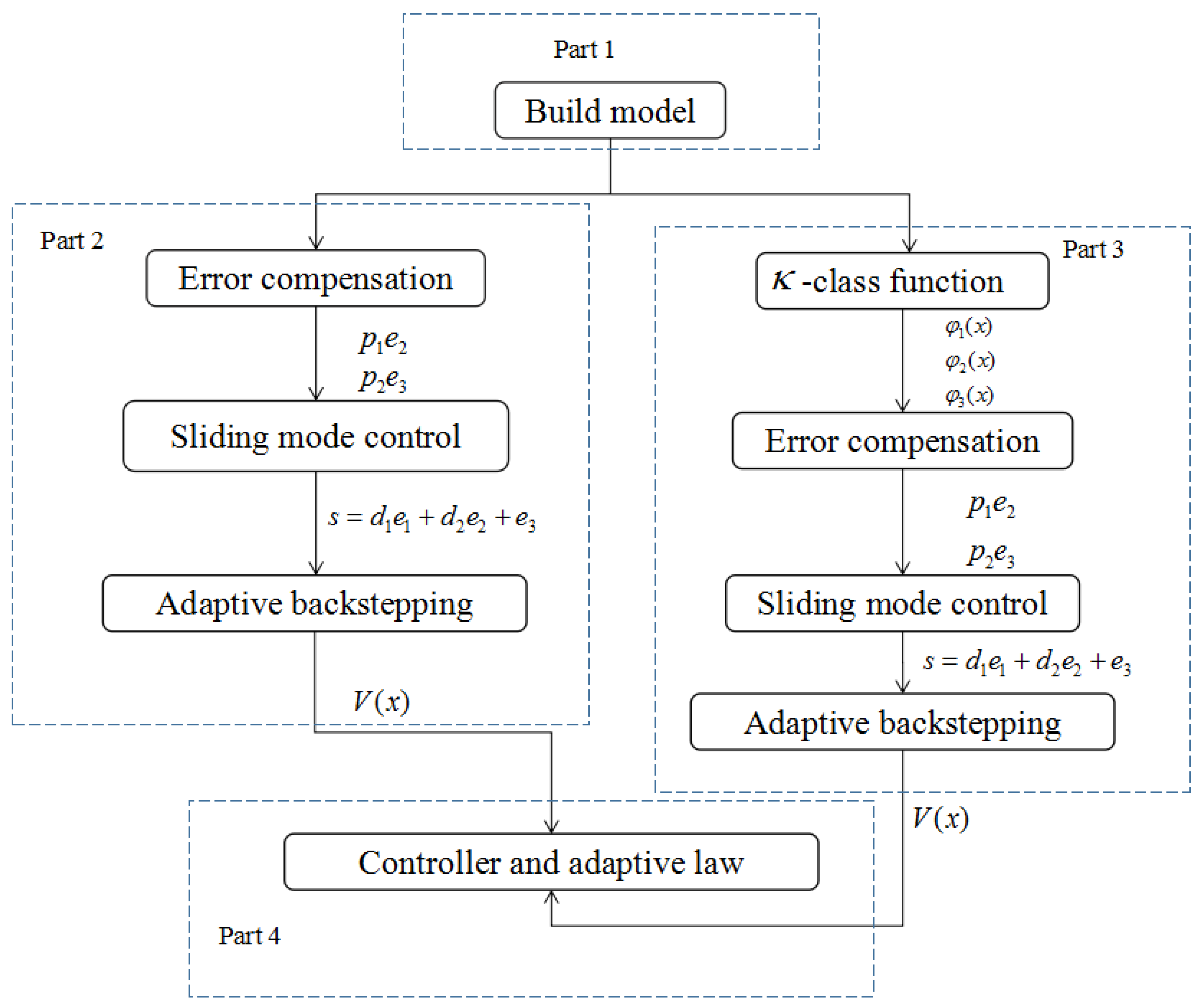
Our control object is designing an adaptive backstepping controller u to make the system stable. This paper researches the nonlinear controller and a parameter updating law for the single machine bus system with SVC. Using the improved ABEC method improves the external disturbances. To get a higher control accuracy for internal parameters perturbations, we put sliding mode control based on error compensation into the traditional adaptive backstepping method. Finally, the three methods are compared by simulation. The structure diagram of SVC system is shown in Figure 2.

3. Design of Adaptive Backstepping Controller Based on Error Compensation

The basic principle of backstepping is to decompose the system into subsystems of n which do not exceed the order of the system. First, we design a part of the Lyapunov function and virtual variables for each subsystem. Then, we can back to the whole system while each subsystem is stable. Finally a nonlinear controller is designed to stabilize the system. Because there is an error between theory and real engineering, this section will consider the influence of error. We will put error compensation into the traditional adaptive backstepping method. The following four steps are designed for backstepping controller.

Definition 1.

For system (2), we select $x_2^{*}$ and $x_3^{*}$ as the virtual stabilization functions. Then, we can obtain error variables $e_i$, i = 1,2,3, as shown by the following equations:

$$\begin{array}{ccc}\hfill e_1& =& x_1\hfill \\ \hfill e_2& =& x_2-x_2^{*}\hfill \\ \hfill e_3& =& x_3-x_3^{*}\hfill \end{array}$$

(3)

Step 1: Firstly, choose the virtual control of $x_2$ as $x_2^{*}$,

$$\begin{array}{c}\hfill x_2^{*}=-({\phi }_1(|e_1|)+c_1)e_1-p_1{e}_2\end{array}$$

(4)

where $c_1$ is a positive constant, ${\phi }_1(·)$ is a class-$\kappa$ function to be designed, and $p_1{e}_2$ is an error compensation to eliminate system shake problem. Then, based on Definition 1, getting

$$\begin{array}{c}\hfill \dot{e_1}=-({\phi }_1(|e_1|)+c_1)e_1+(1-p_1)e_2\end{array}$$

(5)

Choose the first storage Lyapunov function

$$\begin{array}{c}\hfill V_1=\frac{1}{2}{e}_1^2\end{array}$$

(6)

thus, the derivative of $V_1$ is

$$\begin{array}{c}\hfill \dot{V_1}=-({\phi }_1(|e_1|)+c_1)e_1^2+(1-p_1)e_1{e}_2\end{array}$$

(7)

Select ${\phi }_1(·)$ as ${\phi }_1(|e_1|)=\frac{1}{3}{\epsilon }_1{e}_1^2$, where ${\epsilon }_1$ is a positive constant. Absolutely, when $e_2=0$, there is $\dot{V_1}<0$, satisfying the stability condition.

Step 2: Choose a Lyaponov function

$$\begin{array}{c}\hfill V_2=V_1+\frac{1}{2}{e}_2^2\end{array}$$

(8)

we know,

$$\begin{array}{ccc}\hfill \dot{e_2}& =& \dot{x_2}-\dot{x_2^{*}}\hfill \\ & =& \theta x_2+a_0-k(x_3+y)sin(x_1+{\delta }_0)+{\epsilon }_1{e}_1^2{x}_2+c_1{x}_2+p_1\dot{e_2}\hfill \end{array}$$

(9)

then result,

$$\begin{array}{ccc}\hfill \dot{e_2}& =& \dot{x_2}-\dot{x_2^{*}}\hfill \\ & =& \frac{1}{1-p_1}[\theta x_2+a_0-k(x_3+y)sin(x_1+{\delta }_0)+c_1{x}_2+{\epsilon }_1{e}_1^2{x}_2]\hfill \end{array}$$

(10)

The derivative of $V_2$ is

$$\begin{array}{ccc}\hfill \dot{V_2}& =& \dot{V_1}+e_1{e}_2\hfill \\ & =& -({\phi }_1(|e_1|)+c_1)e_1^2+\frac{1}{1-p_1}[{(1-p_1)}^2{e}_1+\theta x_2+a_0-k(x_3+y)sin(x_1+{\delta }_0)+c_1{x}_2+{\epsilon }_1{e}_1^2{x}_2]\hfill \end{array}$$

(11)

Moreover, by Definition 1: $e_3=x_3-x_3^{*}$, choose virtual stabilization function:

$$\begin{array}{ccc}\hfill x_3^{*}& =& \frac{1}{ksin(x_1+{\delta }_0)}[{(1-p_1)}^2{e}_1+\widehat{\theta }{x}_2+a_0+c_1{x}_2+({\phi }_2(|e_2|)+c_2)e_2+p_2{e}_3+{\epsilon }_1{e}_1^2{x}_2]-y\hfill \end{array}$$

(12)

among them $c_2,p_2$ are constants, and ${\phi }_2(·)$ is a class-$\kappa$ function to be designed. Then selecting ${\phi }_2(·)$ as ${\phi }_2(|e_2|)=\frac{1}{3}{\epsilon }_2{e}_2^2$, where ${\epsilon }_2$ is a positive constant, $\widehat{\theta }$ is the estimate of $\theta$, $\tilde{\theta }$ is estimated error and $\tilde{\theta }=\theta -\widehat{\theta }$, thus,

$$\begin{array}{ccc}\hfill \dot{V_2}& =& -({\phi }_1(|e_1|)+c_1)e_1^2+\frac{e_2}{1-p_1}[\tilde{\theta }{x}_2-({\phi }_2(|e_2|)+c_2)e_2-p_2{e}_3-ksin(x_1+{\delta }_0)e_3]\hfill \end{array}$$

(13)

Step 3: For the whole system (2), select the new Lyapunov function

$$\begin{array}{c}\hfill V=V_2+\frac{1}{2}{e}_3^2+\frac{1}{2\rho }{\tilde{\theta }}^2\end{array}$$

(14)

where $\rho >0$ is given adaptive gain parameter, while

$$\begin{array}{ccc}\hfill \dot{e_3}& =& \dot{x_3}-\dot{x_3^{*}}\hfill \\ & =& \frac{ksin(x_1+{\delta }_0)}{ksin(x_1+{\delta }_0)+p_2}\{-\frac{1}{T}{x}_3+\frac{1}{T}u-\frac{1}{ksin(x_1+{\delta }_0)}[{(1-p_1)}^2{x}_2+\dot{\widehat{\theta }}{x}_2+2{\epsilon }_1{e}_1{x}_2^2\hfill \\ & +& \frac{1}{1-p_1}({\epsilon }_2{e}_2^2+c_2)({\epsilon }_1{e}_1^2{x}_2+c_1{x}_2)+(\widehat{\theta }+c_1+\frac{c_2}{1-p_1}+{\epsilon }_1{e}_1^2+\frac{{\epsilon }_2{e}_2^2}{1-p_1})(\theta x_2\hfill \\ & +& a_0-k(x_3+y)sin(x_1+{\delta }_0))]+\frac{cos(x_1+{\delta }_0)x_2}{ksi{n}^2(x_1+{\delta }_0)}[{(1-p_1)}^2{e}_1+\widehat{\theta }{x}_2\hfill \\ & +& a_0+{\epsilon }_1{e}_1^2{x}_2+c_1{x}_2+({\phi }_2(|e_2|)+c_2)e_2+p_2{e}_3]\}\hfill \end{array}$$

(15)

where $p_2{e}_3$ is error compensation term, it can compensate the influence of unknown error in the process of dynamic stability. Since $\theta =\widehat{\theta }+\tilde{\theta }$, the derivative of V is:

$$\begin{array}{ccc}\hfill \dot{V}& =& -({\phi }_1(|e_1|)+c_1)e_1^2-\frac{1}{1-p_1}({\phi }_2(|e_2|)+c_2)e_2^2+\frac{e_2}{1-p_1}\tilde{\theta }{x}_2-\frac{1}{\rho }\tilde{\theta }\dot{\widehat{\theta }}-\frac{e_3\tilde{\theta }{x}_2}{ksin(x_1+{\delta }_0)+p_2}(\widehat{\theta }+{\epsilon }_1{e}_1^2\hfill \\ & +& c_1+\frac{{\epsilon }_2{e}_2^2}{1-p_1}+\frac{c_2}{1-p_1})+\frac{ksin(x_1+{\delta }_0)e_3}{ksin(x_1+{\delta }_0)+p_2}\{-\frac{ksin(x_1+{\delta }_0)+p_2}{1-p_1}{e}_2+\frac{1}{T}u-\frac{1}{T}{x}_3-\frac{1}{ksin(x_1+{\delta }_0)}[{(1-p_1)}^2{x}_2\hfill \\ & +& \dot{\widehat{\theta }}{x}_2+2{\epsilon }_1{e}_1{x}_2^2+\frac{1}{1-p_1}({\epsilon }_2{e}_2^2+c_2)({\epsilon }_1{e}_1^2{x}_2+c_1{x}_2)+(\widehat{\theta }+c_1+\frac{c_2}{1-p_1}+{\epsilon }_1{e}_1^2+\frac{{\epsilon }_2{e}_2^2}{1-p_1})(\widehat{\theta }{x}_2\hfill \\ & +& a_0-k(x_3+y)sin(x_1+{\delta }_0))]+\frac{cos(x_1+{\delta }_0)x_2}{ksi{n}^2(x_1+{\delta }_0)}[{(1-p_1)}^2{e}_1+\widehat{\theta }{x}_2+a_0+{\epsilon }_1{e}_1^2{x}_2\hfill \\ & +& c_1{x}_2+({\phi }_2(|e_2|)+c_2)e_2+p_2{e}_3]\}\hfill \end{array}$$

(16)

Considering (17), get the parameters replacement law

$$\begin{array}{ccc}\hfill \dot{\widehat{\theta }}& =& \rho [\frac{e_2}{1-p_2}-\frac{e_3}{ksin(x_1+{\delta }_0)+p_2}(\widehat{\theta }+{\epsilon }_1{e}_1^2+c_1+\frac{{\epsilon }_2{e}_2^2}{1-p_1}+\frac{c_2}{1-p_1})]x_2\hfill \end{array}$$

(17)

Then

$$\begin{array}{ccc}\hfill \dot{V}& =& -({\phi }_1(|e_1|)+c_1)e_1^2-\frac{1}{1-p_1}({\phi }_2(|e_2|)+c_2)e_2^2-({\phi }_3(|e_3|)+c_3)e_3^2\hfill \end{array}$$

(18)

where ${\phi }_3(·)$ is a class-$\kappa$ function to be designed. Then we can select ${\phi }_3(|e_3|)=\frac{1}{3}{\epsilon }_3{e}_3^2$, and ${\epsilon }_3$ is a positive constant. If there exist new control parameters $p_i$ and constant $c_i$,$0<p_i,c_i<1$, it is clearly, getting $\dot{V}<0$ by (19).

Step 4: Finally, considering the control problem based on Section 2, an adaptive backstepping controller u can be got, as the following shown. The control law u and parameters replacement law $\widehat{\theta }$ based on adaptive backstepping controller of SVC system are follows:

$$\begin{array}{ccc}\hfill u& =& T\{\frac{ksin(x_1+{\delta }_0)+p_2}{1-p_1}{e}_2+\frac{1}{T}{x}_3+\frac{1}{ksin(x_1+{\delta }_0)}[{(1-p_1)}^2{x}_2+\dot{\widehat{\theta }}{x}_2+2{\epsilon }_1{e}_1{x}_2^2+\frac{1}{1-p_1}({\epsilon }_2{e}_2^2+c_2)({\epsilon }_1{e}_1^2{x}_2\hfill \\ & +& c_1{x}_2)+(\widehat{\theta }+c_1+\frac{c_2}{1-p_1}+{\epsilon }_1{e}_1^2+\frac{{\epsilon }_2{e}_2^2}{1-p_1})(\widehat{\theta }{x}_2+a_0-k(x_3+y)sin(x_1+{\delta }_0))]\hfill \\ & -& \frac{cos(x_1+{\delta }_0)x_2}{ksi{n}^2(x_1+{\delta }_0)}[{(1-p_1)}^2{e}_1+\widehat{\theta }{x}_2+a_0+{\epsilon }_1{e}_1^2{x}_2+c_1{x}_2+({\phi }_2(|e_2|)+c_2)e_2+p_2{e}_3]\hfill \\ & -& \frac{ksin(x_1+{\delta }_0)+p_2}{ksin(x_1+{\delta }_0)}({\phi }_3(|e_3|)+c_3)e_3\}\hfill \end{array}$$

(19)

The closed-loop system under the new coordinates $(e_1,e_2,e_3)$ is as follows:

$$\begin{array}{ccc}\hfill \dot{e_1}& =& -({\phi }_1(|e_1|)+c_1)e_1+(1-p_1)e_1{e}_2\hfill \\ \hfill \dot{e_2}& =& \frac{1}{1-p_1}[\tilde{\theta }{x}_2-{(1-p_1)}^2{e}_1-({\phi }_2(|e_2|)+c_2)e_2-p_2{e}_3-ksin(x_1+{\delta }_0)e_3]\hfill \\ \hfill \dot{e_3}& =& \frac{ksin(x_1+{\delta }_0)}{1-p_1}{e}_2-\frac{1}{ksin(x_1+{\delta }_0)+p_2}(\widehat{\theta }+{\epsilon }_1{e}_1^2+c_1+\frac{{\epsilon }_2{e}_2^2}{1-p_1}+\frac{c_2}{1-p_1})\tilde{\theta }{x}_2-({\phi }_3(|e_3|)+c_3)e_3\hfill \end{array}$$

(20)

Theorem 1.

When we consider the model of SVC system (1) under the influence of controller u (19) and parameters $\widehat{\theta }$ (17), the closed-loop system (20) is asymptotically stable nearby the origin.

Proof. 

By (25), we know $V(t)\le V(0)$. Namely, $e_1,e_2,x_1,x_2$ are bounded. Then we define $\mathsf{\Gamma }=-\dot{V},{\int }_0^t\mathsf{\Gamma }(\tau )d\tau =V(0)-V(t)$. Because V(0) is bounded, V(t) is also decreasing and bounded, we know that $\underset{t\to \infty }{lim}{\int }_0^t\mathsf{\Gamma }(\tau )d\tau <\infty$. In addition, $\dot{\mathsf{\Gamma }}$ is bounded, thus, $\underset{t\to \infty }{lim}\mathsf{\Gamma }=0$ is proved by Barbalat lemma. When $t\to \infty$, there are $e_1\to 0,e_2\to 0,x_1\to 0,x_2\to 0$. Based on the definitions of $x_1,x_2,x_3$ and $x_2^{*},x_3^{*}$, we know that $e_3\to 0$, $x_3$ is also bounded. ☐

Remark 2.

If $\delta =k\pi ,k=0,1,2,3\dots$, then $sin(x_1+{\delta }_0)=0$, the power system will be lost stability and there is no longer normal operation. Fortunately, in support of the normal conditions in the system $0<\delta <\pi$, $sin(x_1+{\delta }_0)\ne 0$ can be guaranteed.

Remark 3.

When the coefficient of error compensation $p_1,p_2=0$, the ABSMVCEC method changes into the traditional backstepping control method. In other words, the traditional backstepping method is a special case of Theorem 1.

Remark 4.

We take a class-κ function ${\phi }_i(·)$, where $i=1,2,\dots n$, during the process of recursive design of update law. By the function of ${\phi }_i(·)$ we can speed up the convergence rate in error. But error is decrease with the increase of time, $\dot{V}$ becomes the traditional adaptive backstepping gradually.

Remark 5.

In the improved adaptive backstepping method above, if ${\phi }_i(·)\equiv 0$, it equivalents to the traditional methods.

4. Design of Adaptive Backstepping Sliding Mode Variable Structure Controller Based on Error Compensation

To get a higher control accuracy for internal parameters perturbations, we put sliding mode variable structure control based on error compensation into the traditional adaptive backstepping method.

The ABSMVCEC method is the same as the chapters mentioned before, thus we start from step 3 to introduce the improved method.

Step 3: Choose the sliding mode surface $s=d_1{e}_1+d_2{e}_2+e_3=0$, $d_1$ and $d_2$ are constants respectively. The whole system Lyapunove function is given by

$$\begin{array}{c}\hfill V=V_2+\frac{1}{2}{s}^2+\frac{1}{2\rho }{\tilde{\theta }}^2\end{array}$$

(21)

while noting that $\dot{s}=d_1\dot{e_1}+d_2\dot{e_2}+\dot{e_3}$. The derivative of V is

$$\begin{array}{c}\hfill \dot{V}=\dot{V_2}+s\dot{s}-\frac{1}{\rho }\tilde{\theta }\dot{\widehat{\theta }}\end{array}$$

(22)

since $\theta =\widehat{\theta }+\tilde{\theta }$ and $e_3=s-d_1{e}_1-d_2{e}_2$, therefore,

$$\begin{array}{ccc}\hfill \dot{V}& =& -(-({\phi }_1(|e_1|)+c_1)-\frac{ksin(x_1+{\delta }_0)+p_2}{2(1-p_1)}{d}_1)e_1^2-[(\frac{1}{1-p_1}({\phi }_2(|e_2|)+c_2)-\frac{ksin(x_1+{\delta }_0)+p_2}{2(1-p_1)}{d}_1\hfill \\ & -& \frac{ksin(x_1+{\delta }_0)+p_2}{1-p_1}{d}_2]e_2^2-\frac{ksin(x_1+{\delta }_0)+p_2}{2(1-p_1)}{d}_1{(e_1-e_2)}^2+\frac{e_2}{1-p_1}\tilde{\theta }{x}_2-\frac{1}{\rho }\tilde{\theta }\dot{\widehat{\theta }}+\frac{d_{2}s}{1-p_1}\tilde{\theta }{x}_2\hfill \\ & -& \frac{s}{ksin(x_1+{\delta }_0)+p_2}(\widehat{\theta }+{\epsilon }_1{e}_1^2+c_1+\frac{{\epsilon }_2{e}_2^2}{1-p_1}+\frac{c_2}{1-p_1})\tilde{\theta }{x}_2+s\{-\frac{e_2}{1-p_1}{p}_2-\frac{ksin(x_1+{\delta }_0)}{1-p_1}{e}_2\hfill \\ & +& d_1{x}_2+\frac{d_2}{1-p_1}[\widehat{\theta }{x}_2+a_0-k(x_3+y)sin(x_1+{\delta }_0)+c_1{x}_2+{\epsilon }_1{e}_1^2{x}_2]\hfill \\ & +& \frac{ksin(x_1+{\delta }_0)}{ksin(x_1+{\delta }_0)+p_2}\{-\frac{1}{T}{x}_3+\frac{1}{T}u+\frac{cos(x_1+{\delta }_0)x_2}{ksi{n}^2(x_1+{\delta }_0)}[{(1-p_1)}^2{e}_1+\widehat{\theta }{x}_2+a_0\hfill \\ & +& {\epsilon }_1{e}_1^2{x}_2+c_1{x}_2+({\phi }_2(|e_2|)+c_2)e_2+p_2{e}_3]-\frac{1}{ksin(x_1+{\delta }_0)}[{(1-p_1)}^2{x}_2\hfill \\ & +& \dot{\widehat{\theta }}{x}_2+2{\epsilon }_1{e}_1{x}_2^2+\frac{1}{1-p_1}({\epsilon }_2{e}_2^2+c_2)({\epsilon }_1{e}_1^2{x}_2+c_1{x}_2)+(\widehat{\theta }+c_1+\frac{c_2}{1-p_1}+{\epsilon }_1{e}_1^2\hfill \\ & +& \frac{{\epsilon }_2{e}_2^2}{1-p_1})(\widehat{\theta }{x}_2+a_0-k(x_3+y)sin(x_1+{\delta }_0))]\}\}\hfill \end{array}$$

(23)

The parameter replacement law is that

$$\begin{array}{ccc}\hfill \dot{\widehat{\theta }}& =& \rho [\frac{e_2}{1-p_1}+\frac{d_{2}s}{1-p_1}-\frac{s}{ksin(x_1+{\delta }_0)+p_2}(\widehat{\theta }+{\epsilon }_1{e}_1^2+c_1+\frac{{\epsilon }_2{e}_2^2}{1-p_1}+\frac{c_2}{1-p_1})]x_2\hfill \end{array}$$

(24)

Then

$$\begin{array}{ccc}\hfill \dot{V}& =& -(-({\phi }_1(|e_1|)+c_1)-\frac{ksin(x_1+{\delta }_0)+p_2}{2(1-p_1)}{d}_1)e_1^2-[(\frac{1}{1-p_1}({\phi }_2(|e_2|)+c_2)-\frac{ksin(x_1+{\delta }_0)+p_2}{2(1-p_1)}{d}_1\hfill \\ & -& \frac{ksin(x_1+{\delta }_0)+p_2}{1-p_1}{d}_2]e_2^2-\frac{ksin(x_1+{\delta }_0)+p_2}{2(1-p_1)}{d}_1{(e_1-e_2)}^2-({\phi }_3(|e_3|)+\beta )s^2\hfill \end{array}$$

(25)

Select the same class-$\kappa$ function ${\phi }_1(·)$, ${\phi }_2(·)$ as ${\phi }_1(|e_1|)=\frac{1}{3}{\epsilon }_1{e}_1^2$, ${\phi }_2(|e_2|)=\frac{1}{3}{\epsilon }_2{e}_2^2$, select ${\phi }_3(·)$ as ${\phi }_3(|e_3|)=\frac{1}{3}{\epsilon }_3{e}_3^2$, where ${\epsilon }_1,{\epsilon }_2,{\epsilon }_3>0$.

Step 4: Obviously, $\dot{V}<0$ by (25), then an adaptive backstepping controller u can be got according to Section 2. We can choose the proper parameters $c_i,d_i,p_i,i=1,2$, which meet conditions

(1)

$({\phi }_1(|e_1|)+c_1)-\frac{ksin(x_1+{\delta }_0)+p_2}{2(1-p_1)}{d}_1\ge 0$

(2)

$\frac{1}{1-p_1}({\phi }_2(|e_2|)+c_2)-\frac{ksin(x_1+{\delta }_0)+p_2}{2(1-p_1)}{d}_1-\frac{ksin(x_1+{\delta }_0)+p_2}{1-p_1}{d}_2\ge 0$

(3)

$\frac{ksin(x_1+{\delta }_0)+p_2}{2(1-p_1)}{d}_1\ge 0$

We know, $\beta >0$ is a positive parameter of the sliding mode, and the other parameter variables should be given according to control requirements.

The control law u based on ABSMVCEC method is as follows:

$$\begin{array}{ccc}\hfill u& =& T\{[\frac{ksin(x_1+{\delta }_0)+p_2}{ksin(x_1+{\delta }_0)}[\frac{ksin(x_1+{\delta }_0)+p_2}{1-p_1}{e}_2-d_1{x}_2-\frac{d_2}{1-p_1}[\widehat{\theta }{x}_2+a_0-k(x_3+y)sin(x_1+{\delta }_0)+{\epsilon }_1{e}_1^2{x}_2\hfill \\ & +& c_1{x}_2]]+\frac{1}{T}{x}_3-\frac{cos(x_1+{\delta }_0)x_2}{ksi{n}^2(x_1+{\delta }_0)}[{(1-p_1)}^2{e}_1+\widehat{\theta }{x}_2+a_0+{\epsilon }_1{e}_1^2{x}_2+c_1{x}_2+({\phi }_2(|e_2|)+c_2)e_2+p_2{e}_3]\hfill \\ & +& \frac{1}{ksin(x_1+{\delta }_0)}[{(1-p_1)}^2{x}_2+\dot{\widehat{\theta }}{x}_2+2{\epsilon }_1{e}_1{x}_2^2+\frac{1}{1-p_1}({\epsilon }_2{e}_2^2+c_2)({\epsilon }_1{e}_1^2{x}_2+c_1{x}_2)+(\widehat{\theta }+c_1+\frac{c_2}{1-p_1}\hfill \\ & +& {\epsilon }_1{e}_1^2+\frac{{\epsilon }_2{e}_2^2}{1-p_1})(\widehat{\theta }{x}_2+a_0-k(x_3+y)sin(x_1+{\delta }_0))]-\frac{ksin(x_1+{\delta }_0)+p_2}{ksin(x_1+{\delta }_0)}({\phi }_3(|e_3|)+\beta )s\}\hfill \end{array}$$

(26)

The closed-loop system under the new coordinates $(e_1,e_2,e_3)$ are

$$\begin{array}{ccc}\hfill \dot{e_1}& =& -({\phi }_1(|e_1|)+c_1)e_1+(1-p_1)e_1{e}_2\hfill \\ \hfill \dot{e_2}& =& \frac{1}{1-p_1}[\tilde{\theta }{x}_2-{(1-p_1)}^2{e}_1-({\phi }_2(|e_2|)+c_2)e_2-p_2{e}_3-ksin(x_1+{\delta }_0)e_3]\hfill \\ \hfill \dot{e_3}& =& \frac{ksin(x_1+{\delta }_0)+p_2}{1-p_1}{e}_2-d_1{x}_2-\frac{d_2}{1-p_1}[\widehat{\theta }{x}_2+a_0-k(x_3+y)sin(x_1+{\delta }_0)+{\epsilon }_1{e}_1^2{x}_2+c_1{x}_2]\hfill \\ & -& \frac{1}{ksin(x_1+{\delta }_0)+p_2}(\widehat{\theta }+{\epsilon }_1{e}_1^2+c_1+\frac{{\epsilon }_2{e}_2^2}{1-p_1}+\frac{c_2}{1-p_1})\tilde{\theta }{x}_2-({\phi }_3(|e_3|)+\beta )s\hfill \end{array}$$

(27)

Theorem 2.

When we consider mode for the valve control system (1) with its equivalent from (2), the closed-loop error system (27) is asymptotically stable nearby the origin under the influence of the control law u (26).

Proof. 

By (25), we know $V(t)\le V(0)$. Namely, $e_1,e_2,x_1,x_2$ are bounded. Then we define $\mathsf{\Gamma }=-\dot{V},{\int }_0^t\mathsf{\Gamma }(\tau )d\tau =V(0)-V(t)$. Because V(0) is bounded, V(t) is also decreasing and bounded, we know that $\underset{t\to \infty }{lim}{\int }_0^t\mathsf{\Gamma }(\tau )d\tau <\infty$. In addition, $\dot{\mathsf{\Gamma }}$ is bounded, thus, $\underset{t\to \infty }{lim}\mathsf{\Gamma }=0$ is proved by Barbalat lemma. When $t\to \infty$, there are $e_1\to 0,e_2\to 0,x_1\to 0,x_2\to 0$. Based on the definitions of $x_1,x_2,x_3$ and $x_2^{*},x_3^{*}$, we know that $e_3\to 0$, $x_3$ is also bounded. ☐

Remark 6.

We add the parameter ${\epsilon }_i,i=1,2,3$ in the design process. We could select the smaller parameter ${\epsilon }_i$ when the error is larger, thus it makes the controller gain does not increase a lot. In order to improve the transient performance advantage, we could select the bigger ${\epsilon }_i$ when the error is smaller. That is to say, the corresponding speed of the system can be increased or decreased by adjusting the gain parameter ${\epsilon }_i$.

Remark 7.

When the parameters $p_1,p_2=0,d_1,d_2=0,{\epsilon }_1=0,{\epsilon }_2=0,{\epsilon }_3=0$, the ABSMVCEC method becomes the traditional backstepping control. In other words, the traditional backstepping sliding mode method is a special case of Theorem 2.

5. Simulation

In order to verify the effectiveness of the improved method, we have carried on the simulation to the system. These are system parameters which are chosen from [17]: $c_i(i=1,2,3)$ is positive constant, taken $c_1=2.5;c_2=2;c_3=2;$ $p_i(i=1,2)$ is a positive error constant, taken $p_1=0.85;p_2=0.45;$ $\rho$ is adaptive gain parameter, taken $\rho =1;$ T is the inertial time constant, taken $T=0.02;$ V is infinite bus voltage, taken $V=1$; E is transient electric potential, $E=0.05;$ H is moment of inertia, $H=20;$ w is speed of the generator rotor, $y_{svc}$ is the susceptance of the overall system, $\delta$ is the angle of the generator rotor, and $w_0,y_0,{\theta }_0$ is the work point when the system is stable, taken $w_0=314;y_0=0.814;{\theta }_0=57$.

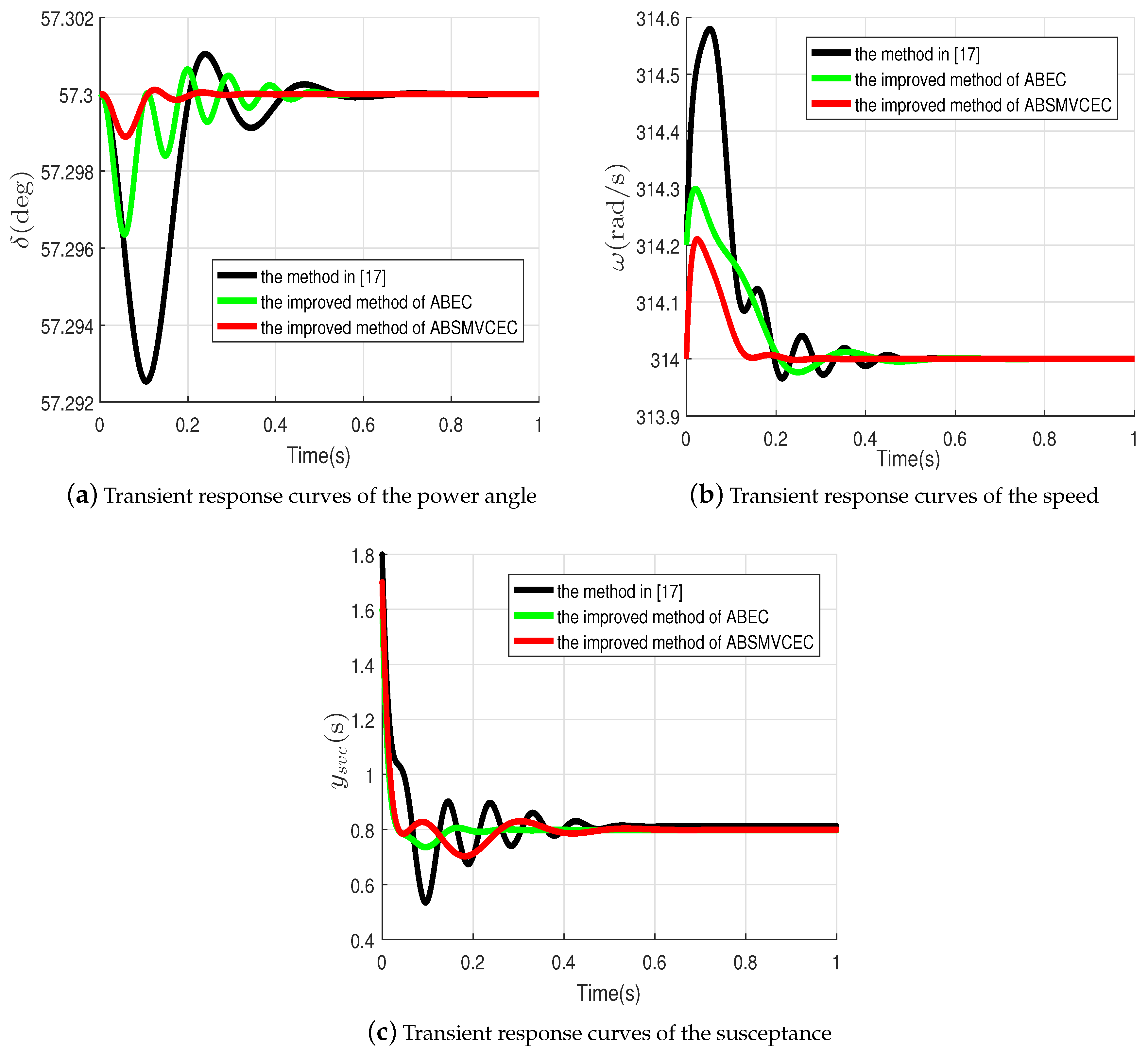
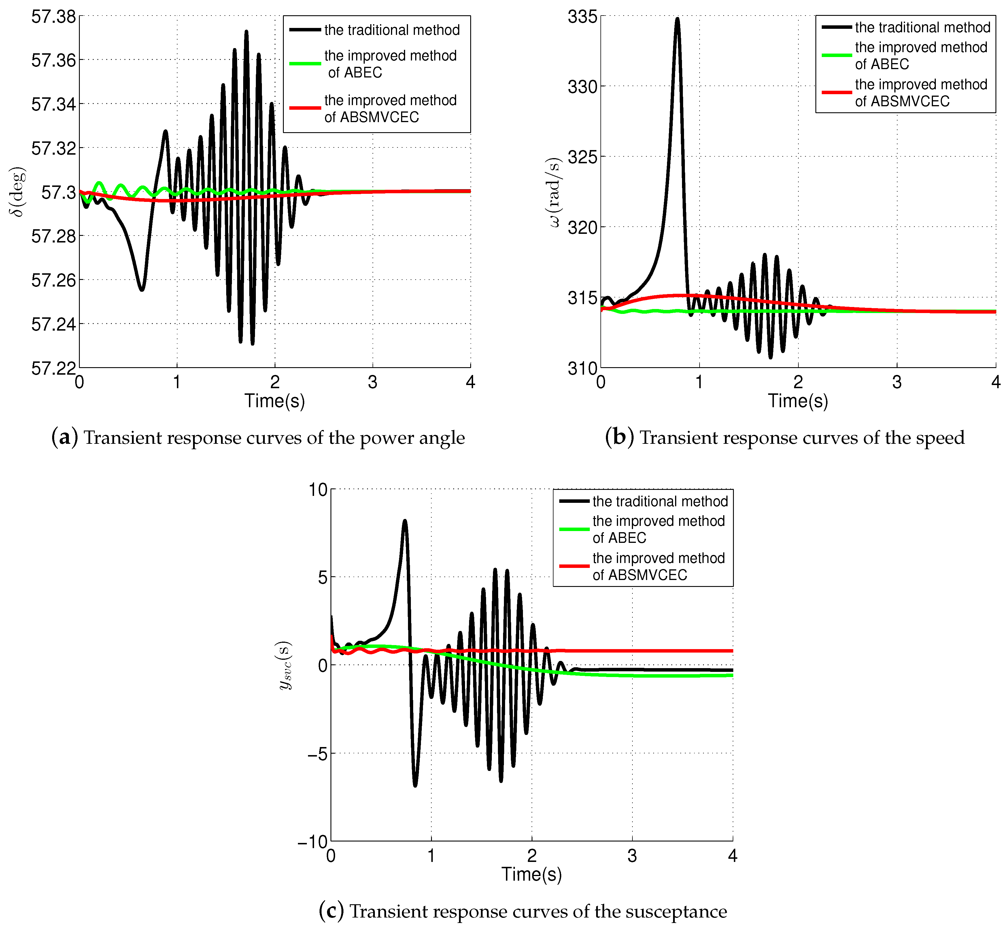
As shown in Figure 3 and Figure 4, the black line represents the traditional adaptive backstepping method, the green line represents the ABEC method, and the red line represents the ABSMVCEC method.

As shown in Figure 3a, setting the initial value of the power angle to 57.3, we can see the power angle ${\delta }_0$ is 57.3 when the system is stable from Figure 3a. That is to say $x_1$ gradually tends to 0, thus the error gradually tends to 0, and it makes the system stable. We can see the improved ABSMVCEC method makes transient power angle performance better compared with the method of adaptive backstepping in [17] and the improved ABEC method from Figure 3a. In addition, the improved method of ABSMVCEC has faster convergence rate and smaller amplitude of vibration compared with the other two methods. In addition, we can see from Figure 4a that the effect of the power angle $\delta$ is also the same under large perturbations. When there is a large perturbation, the traditional method fluctuates greatly, but the improved method can resist the perturbation very well.

As shown in Figure 3b, we set the initial value of the speed of the generator rotor to 314, and we can see the operating point of the power system ($w_0$) is gradually tends to 314, that is to say $x_2$ gradually tends to 0, thus error gradually tends to 0, the system gradually stable. It is clearly to see that three controllers settle down to their steady state values. However, the third method can make the system stable more quickly, meanwhile, the transient stability is smaller and smoother than above two methods. In a word, the third method shows a faster convergence speed and a better transient performance. In addition, we can see from Figure 4b that the effect of the speed $\omega$ is also the same under large perturbations. When there is a large perturbation, the traditional method fluctuates greatly, but the improved method can resist the perturbation very well.

As shown in Figure 3c, the susceptance $y_{svc}$ tends to 0.8, stabile basically. In addition, we can see the three methods all can get the system stable. It is obviously that the ABSMVCEC method has a faster convergence speed and brings a better steady state. Also, we can see from Figure 4c that the effect of the susceptance $y_{svc}$ is also the same under large perturbations. When there is a large perturbation, the traditional method fluctuates greatly, but the improved method can resist the perturbation very well.

6. Conclusions

This paper investigates the nonlinear controller for SVC system with the ABSMVCEC method. From the result of simulations, we can see that the two new methods all have better influences on the nonlinear power system; in particular, the ABSMVCEC method is more effective in improving the transient stability. In order to avoid one-sided pursuit of transient response speed and make the controller gain too heavy for implementation, this paper designs parameters ${\epsilon }_i$, $i=1,2,3$, to adjust the contradiction.

References

- Benidris, M.; Elsaiah, S.; Sulaeman, S.; Mitra, J. Transient Stability of Distributed Generators in the Presence of Energy Storage Devices. In Proceedings of the 44th IEEE North American Power Symposium, Champaign, IL, USA, 9–11 September 2012. [Google Scholar]
- Caciotta, M.; Leccese, F.; Trifiro, A. From power quality to perceived power quality. In Proceedings of the IASTED International Conference on Energy and Power Systems, Chiang Mai, Thailand, 29–31 March 2006; pp. 94–102. [Google Scholar]
- De Araujo, V.V.; Simas Filho, E.F.; Oliveira, A.; de Oliveira, W.L.A.; Esteves, L.T.C. Integrated circuit for real-time poly-phase power quality monitoring. Microelectron. J. 2018, 79, 57–63. [Google Scholar] [CrossRef]
- Kundur, P. Power System Stability and Control; Et Power Electronics; McGraw-Hill Education: New York, NY, USA, 2007; Volume 7, pp. 100–103. [Google Scholar]
- Su, J.; Chen, C. Study on SVC control for power system with nonlinear loads. Autom. Electri. Power Syst. 2002, 26, 12–15. [Google Scholar]
- Li, S.; Su, Z. Static state feedback control for saddle-node bifurcation in a simple power system. In Proceedings of the International Conference on Power Electronics and Intelligent Transportation System, Shenzhen, China, 19–20 December 2010; pp. 158–160. [Google Scholar]
- Hwang, Y.H.; Park, K.K.; Yang, H.W. Robust adaptive backstepping control for efficiency optimization of induction motors with uncertainties. In Proceedings of the ieee International Symposium on Industrial Electronics, Cambridge, UK, 30 June–2 July 2008; pp. 878–883. [Google Scholar]
- Okano, K.; Hagino, K. Adaptive control design approximating solution of Hamilton-Jacobi-Bellman equation for nonlinear strict-feedback system with uncertainties. In Proceedings of the Annual Conference on Sice Conference, Tokyo, Japan, 20–22 August 2008; pp. 204–208. [Google Scholar]
- Modi, P.K.; Singh, S.P.; Sharma, J.D. Fuzzy neural network based voltage stability evaluation of power systems with SVC. Appl. Soft Comput. 2008, 8, 657–665. [Google Scholar] [CrossRef]
- Dimirovski, G.; Yuan, W.; Wen, L. Adaptive Back-Stepping Design of TCSC Robust Nonlinear Control for Power Systems. Intell. Autom. Soft Comput. 2006, 12, 75–87. [Google Scholar] [CrossRef]
- Shang, A.L.; Wang, Z. Adaptive backstepping second order sliding mode control of non-linear systems. Int. J. Model. Identif. Control 2013, 19, 195–201. [Google Scholar] [CrossRef]
- Shi, C.X.; Yang, G.H.; Li, X.J. Robust adaptive backstepping control for hierarchical multi-agent systems with signed weights and system uncertainties. IET Control Theory Appl. 2017, 11, 2743–2752. [Google Scholar] [CrossRef]
- Mitra, A.; Mukherjee, M.; Naik, K. Enhancement of power system transient stability using a novel adaptive backstepping control law. In Proceedings of the Third International Conference on Computer, Communication, Control and Information Technology, West-Bengal, India, 7–8 February 2015; pp. 1–5. [Google Scholar]
- Manosa, V.; Ikhouane, F.; Rodellar, J. Control of uncertain non-linear systems via adaptive backstepping. J. Sound Vib. 2005, 280, 657–680. [Google Scholar]
- Wang, H.M.; Huang, T.L.; Tsai, C.M. Power system stabilizer design using adaptive backstepping controller. In Proceedings of the Fifth International Conference on Power Electronics and Drive Systems, Singapore, 17–20 November 2003. [Google Scholar]
- Benayache, R.; Chrifialaoui, L.; Bussy, P. Adaptive backstepping sliding mode control for hydraulic system without overparametrisation. Int. J. Model. Identif. Control 2012, 16, 60–69. [Google Scholar] [CrossRef]
- Sun, L.-Y. Based on the Backstepping Method of Power System Nonlinear Robust Adaptive Control Design; Northeastern University: Boston, MA, USA, 2009; pp. 50–56. [Google Scholar]
- Zhang, T.; Dong, C. Compound control system design based on adaptive backstepping theory. J. Beijing Univ. Aeronaut. Astronaut. 2013, 39, 902–906. [Google Scholar]
- Mao, J.; Sun, Y.-K.; Wu, G.-Q.; Liu, X.-F. A variable structure robust control method in SVC application for performance improvement. In Proceedings of the 2007 Chinese Control Conference, Harbin, China, 7–11 August 2006; pp. 67–70. [Google Scholar]
- Hagras, A.; Zaid, S.; Ekousy, A.A. Performance comparison of shunt active power filter for interval type-2 fuzzy and adaptive backstepping controllers. Int. J. Model. Identif. Control 2014, 21, 270–287. [Google Scholar] [CrossRef]
- Salma, K.; Nouha, B.; Souhir, S.; Larbi, C.-A.; MBA, K. Transient stability enhancement and voltage regulation in SMIB power system using SVC with PI controller. In Proceedings of the International Conference on Systems and Control, Wuhan, China, 7–9 May 2017; pp. 115–120. [Google Scholar]
- Yimin, L.; Yang, Y.; Li, L. Adaptive Backstepping Fuzzy Control Based on Type-2 Fuzzy System. J. Appl. Math. 2012, 2012, 295–305. [Google Scholar]
- Lin, F.J.; Shen, P.H.; Hsu, S.P. Adaptive backstepping sliding mode control for linear induction motor drive. Proc. Electr. Power Appl. 2002, 149, 184–194. [Google Scholar] [CrossRef]
- Yu, H.; Wang, J.; Deng, B. Adaptive backstepping sliding mode control for chaos synchronization of two coupled neurons in the external electrical stimulation. Commun. Nonlinear Sci. Numer. Simul. 2012, 17, 1344–1354. [Google Scholar] [CrossRef]
- Song, Z.; Sun, K. Adaptive backstepping sliding mode control with fuzzy monitoring strategy for a kind of mechanical system. ISA Trans. 2014, 53, 125–133. [Google Scholar] [CrossRef] [PubMed]
- Zhao, D.; Zou, T.; Li, S. Adaptive backstepping sliding mode control for leader-follower multi-agent systems. Control Theory Appl. IET 2012, 6, 1109–1117. [Google Scholar] [CrossRef]
- Gong, X.; Hou, Z.C.; Zhao, C.J. Adaptive Backstepping Sliding Mode Trajectory Tracking Control for a Quad-rotor. Int. J. Autom. Comput. 2012, 9, 555–560. [Google Scholar] [CrossRef]
- Dong, L.; Tang, W.C. Adaptive backstepping sliding mode control of flexible ball screw drives with time-varying parametric uncertainties and disturbances. ISA Trans. 2014, 53, 110–116. [Google Scholar] [CrossRef] [PubMed]
- Ma, L.; Schilling, K.; Schmid, C. Adaptive Backstepping Sliding Mode Control with Gaussian Networks for a Class of Nonlinear Systems with Mismatched Uncertainties. In Proceedings of the IEEE 2005 and 2005 European Control Conference on Decision and Control, Seville, Spain, 12–15 December 2005; pp. 5504–5509. [Google Scholar]
Figure 1.
Single machine infinite bus system with SVC.
Figure 2.
The structure diagram of SVC system.
Figure 3.
(a–c) are simulation results for the system (1) in small perturbations.
Figure 4.
(a–c) are simulation results for the system (1) in large perturbations.
© 2018 by the authors. Licensee MDPI, Basel, Switzerland. This article is an open access article distributed under the terms and conditions of the Creative Commons Attribution (CC BY) license (http://creativecommons.org/licenses/by/4.0/).
Share and Cite
MDPI and ACS Style
Su, Q.; Dong, F.; Shen, X. Improved Adaptive Backstepping Sliding Mode Control of Static Var Compensator. Energies 2018, 11, 2750. https://doi.org/10.3390/en11102750
AMA Style
Su Q, Dong F, Shen X. Improved Adaptive Backstepping Sliding Mode Control of Static Var Compensator. Energies. 2018; 11(10):2750. https://doi.org/10.3390/en11102750
Chicago/Turabian StyleSu, Qingyu, Fei Dong, and Xueqiang Shen. 2018. "Improved Adaptive Backstepping Sliding Mode Control of Static Var Compensator" Energies 11, no. 10: 2750. https://doi.org/10.3390/en11102750
Note that from the first issue of 2016, this journal uses article numbers instead of page numbers. See further details here.