Analysis of Accuracy Determination of the Seasonal Heat Demand in Buildings Based on Short Measurement Periods


1
Faculty of Energy and Environmental Engineering, The Silesian University of Technology, Konarskiego 20, 44-100 Gliwice, Poland
2
Faculty of Civil Engineering, The Silesian University of Technology, Akademicka 5, 44-100 Gliwice, Poland
*
Author to whom correspondence should be addressed.
Energies 2018, 11(10), 2734; https://doi.org/10.3390/en11102734
Submission received: 26 September 2018
/
Revised: 2 October 2018
/
Accepted: 9 October 2018
/
Published: 12 October 2018
Abstract
:In this paper, we present a multi-variant analysis of the determination of the accuracy of the seasonal heat demand in buildings. The research was based on the linear regression method for data obtained during short periods of measurement. The analyses were carried out using computer simulation, and the numerical models of the multifamily building and school building were used for the simulation. The simulations were performed using the TRNSYS, ESP-r, and CONTAM programs. The multi-zone models of the buildings were validated based on the measurement data. The impact of the building’s parameters (airtightness, insulation, and occupancy schedule) on the determination of the accuracy of the seasonal heat demand was analyzed. The analyses allowed guidelines to be developed for determining the seasonal energy consumption for heating and ventilation based on short periods of heat demand measurements and to determine the optimal duration of the measurement period.
1. Introduction
The directive regarding the energy performance of buildings has introduced the obligation to carry out an energy performance review for new buildings or buildings undergoing thermomodernization, whether being sold or rented [1]. The seasonal heat consumption in buildings (as a strategic element of energy policy) is often predicted using dynamic models that take into account the geometry of the building, its thermal properties, and the existing heating, cooling, ventilation, and air conditioning (HVAC) installations. Modeling appropriate algorithms for the regulation and control of HVAC devices allows for optimization of the energy consumption [2,3,4]. Dynamic methods are accurate but require very detailed data, as well as a large amount of work.
The seasonal heat consumption is the element of the energy characteristic of a building which determines the energy status of that building. In this case, the methods of forecasting seasonal heat consumption should be simple and fast; therefore, static models are used. The energy characteristics, the main component of which is the energy consumption for heating and ventilation in the standard heating season, can be determined by means of a calculation method or by measuring the amount of energy consumed in the actual building. The energy signature method (ES) which represents a static model can be used, based on a linear regression. According to the EN 15603:2008 standard [5] the ES method can be used to monitor the energy consumption in buildings and, additionally, to determine the energy performance of a building. The purpose of linear regression is to find a suitable model and to identify the best-fit regression coefficients, based on the given data, in order to make the estimation error as small as possible. Regression analysis is one of the most commonly used methods to determine the expected value. The standard adopts the following assumptions: Energy consumption for heating purposes is correlated with climatic data within a reasonable period of time, the internal temperature is constant, the main parameter influencing energy consumption is the outside temperature, internal gains are stable, and solar gains are small. The graphical interpretation of the basic ES model is the dependence of the heating power on the outside temperature. For cases of significant solar gains, the standard recommends the use of an adjusted energy signature method: H-m. This is a dependence of the apparent heat loss coefficient of the building H from the meteorological variable m, which is the ratio of solar radiation to the difference between the internal and external temperature. The standard does not specify the minimum duration of the measurements, but it notes that the period should be long enough–several years. If data from a period of less than three years is used to determine the energy performance, the energy consumption must refer to the standard climatic conditions of the building’s location.
The standard states that the averaging period of the data can range from one hour to one week. The integration period depends on the type of building and the conditions occurring therein [6,7]. Castillo et al. [6] studied how it is possible to use the integration period of data averaging (1 to 20 days) with a linear regression-based method. The survey was carried out in a used office room located on the north side of a fully monitored office building, in order to determine the overall heat transfer coefficient UA (W/K). The analysis used hourly recorded survey data from a period of 26 months that was averaged daily. The regression equation refers to the static state, but the applied dynamic integrated approach allowed for the inclusion of the dynamic characteristics of the system concerned in the balance sheet in the established state. Using the heat measurement data supplied by the heating agent for the room, it was noted that the spread in the UA estimates increased when the integration period was over ten days. By taking into account the accumulation of heat in the bulkheads, the degree of airtightness of the heat exchanged with the corridor and the adjacent rooms, as well as the occupancy scheme and the estimated solar gains, the accuracy that was achieved was below 10% for the seven-day integration period of the measurement data. Belussi and Danza [7] noted that the weekly integration period for the estimation of the seasonal heat consumption for heating purposes was sufficient, while daily averaging allowed them to grasp the malfunctioning of the installation. Similar conclusions were obtained from the analysis of simulation results for the heat demand of the multi-family building [8].
Regression-based methods are easier for practical use than methods that use neural networks or simulation methods, as noted in the literature [6,9]. In many of the works, regression methods were used to predict the energy consumption in buildings: A simple linear regression or a multi-criterion regression. Studies have been performed in both small test buildings, as well as in single rooms and large multifamily buildings, or even office buildings, to predict the energy consumption for heating and cooling or to determine the overall heat transfer coefficient of the buildings. Simulation data were used from measurements or from energy bills over a long period of time: From one year to three years.
In Italy, the energy signature method is used in the pre-energy audit to detect problems in the use of energy in the building [7]. The design (DES) and real (RES) energy signatures are then compared. This method was tested on an apartment in a multi-family building, using measurements over the period of one year. The slopes of the straight lines of the RES and DES were comparable but were shifted, which attested to the fact that the coefficient of heat loss was the same, but that the object required modernization to reduce the energy consumption. In turn, in another study [10], the analysis of the real energy consumption of the residential buildings and its comparison with the calculated energy performance was carried out through the energy signature method, by relating the annual delivered energy to the heating degree-days for each analyzed year.
In Sweden, with the energy signature method, the overall heat loss coefficient has been set for more than 100 multi-family buildings based on the monthly energy consumption figures from several years [11]. Further analyses for nine recently built multifamily buildings in Stockholm using the ES method have been described in an article by Sjorgen [12] in which a lumped model was used. Based on the three-year energy consumption data using the linear regression method, the sensitivity of the overall heat loss coefficient of the building was investigated for internal gains and solar and human radiation. Values estimated from October to march on the basis of monthly data were almost insensitive to the coefficient of heat gain, solar radiation, and the input period–one year or more. It should be noted that in both works the analysis was limited to the period from October to March, because during this period the solar heat gains were small and could be neglected. In the article by Vesterberg [13], the linear regression method was used to establish parameters for simulation models (buildings’ transmission losses above ground and ground heat loss) in two monitored multi-family buildings equipped with a ventilation system exhaust, with and without heat recovery. Two different measurement data periods were used, examining the variability of individual parameters according to the difference between the internal and external temperature. A good high value of fit (R2 = 0.96) was obtained. Data from December to February was used, with a period in which there were negligible solar heat gains.
In cases where significant solar radiation occurred during the measurement period, the corrected linear regression model must be applied. This model was proposed in an article by Vesterberg [14], in order to estimate the overall heat loss coefficient of two multi-family buildings, based on measurements over a period of two years. A good consistency was obtained between the results and the simulations that were carried out (<4%). The developed method has widened the possibility of applying linear regression to cases where solar radiation during the heating season is substantial. Another model–IRLS model (iteratively reweighted least squares)–was proposed in the literature [15] for the prediction of the energy consumption of the building, taking into account the following three variables affecting heat consumption: The building’s global heat loss coefficient, south equivalent surface, and the difference between the internal temperature and the solar temperature. The model validation was based on measurements carried out in 17 multi-family buildings. A good correlation was obtained between the values attained from the simulation and the projected values on the basis of the model (R2 = 0.97440). An 11-story building was selected as a case study. The best conformity of the IRLS model, with a measurement of 12%, was achieved by taking into account the heat gains and behavior of the users; without considering these elements, the difference was 35%.
Analysis using a multiple regression method was carried out to predict the energy consumption, which depends on many different parameters. This method is mainly used to determine the building’s parameters early in the design phase. It is an alternative to simulation methods using neural networks as it is known to be less time-consuming and more straightforward. When used, it can indicate which factors contribute to reducing the energy consumption. Research using the multiple regression method, utilizing data derived from the simulation, have been described in the literature [16,17,18]. In the literature [18], the shape of the building and the coefficients of the partitions were optimized for energy consumption. For most cases, the discrepancy obtained from the regression model differed from the simulation results by less than 5%. It has also been investigated [17], how the various factors of the thermal balance of a building affect the level of correlation, in terms of energy, for the heating and cooling of commercial buildings. The structure of the external partitions and occupancy scheme are of the greatest importance. In France, polynomial regression models were used to predict the monthly energy consumption of single-family buildings in temperate climates [19]. A strong relationship between building design and energy consumption has been observed. With a large amount of data, this multiple-regression method gives accurate results–good compatibility of results obtained using the model–with the results from the simulation (up to 5.2%). In China, an energy consumption analysis for office buildings in five climatic zones was conducted using multiple regression models [16]. In the warmer climate, a better correlation of the annual energy consumption with the design parameters studied was achieved. The difference in the predicted and simulated energy consumption was less than 10%.
Multiple regression models were also used to predict the energy consumption in existing office buildings and utilities on the basis of energy bills or measurements performed over a minimum period of one year [20,21,22]. In the banking sector in Spain, energy consumption has been studied according to building construction and climate type [20]. In England [21], based on the measured values of the outside temperature and humidity over the whole year, electricity and gas consumption in supermarkets has been forecast for subsequent years. External air humidity has been found to have little effect on energy consumption. In Singapore, based on a one-year energy bill, using multiple linear regression, the total energy consumption in six office buildings was defined [22]. It has been shown that even in a tropical region, the energy consumption of most buildings depends on the dry bulb temperature and can be anticipated with a confidence level of 90%, only taking into account this variable, when humidity and total solar radiation are omitted.
The work described above did not examine the impact of the time period, from which the data was taken to build the regression model, on the accuracy of the estimated energy consumption.
In the case of buildings with a permanently measured heat preparation system, the consumption values throughout the heating season are available. In contrast, in the case of measurements in non-measured buildings, where measuring devices that are installed only for the measuring period must be used, it is important that the measuring period should be as short as possible due to cost and the nuisance for the users. On the other hand, the aim is to achieve the highest possible accuracy of the determination of seasonal heat consumption on the basis of the measurements. For this reason, this article has analyzed the applicability of the energy signature method based on linear regression to designate the seasonal heat demand for heating and natural ventilation in two types of buildings: Residential and public utility, on the basis of the heat consumption measured in a short period. Three short measuring periods were analyzed and the shortest that was possible to apply, in which an acceptable accuracy of results can be achieved, was indicated.
2. Methods
Studies on multi-variant analysis accuracy, linear regression method, and seasonal heat demand in a building were carried out, based on short-term data of the heating demand.
The analysis was conducted using computer simulations on a residential multi-family building model and a school, see Figure 1. The term “measurement period” has been used in this article to determine the time interval on the basis of which the seasonal heat demand was determined. The impact of the building’s parameters on the archived accuracy was also analyzed.
2.1. Research Site
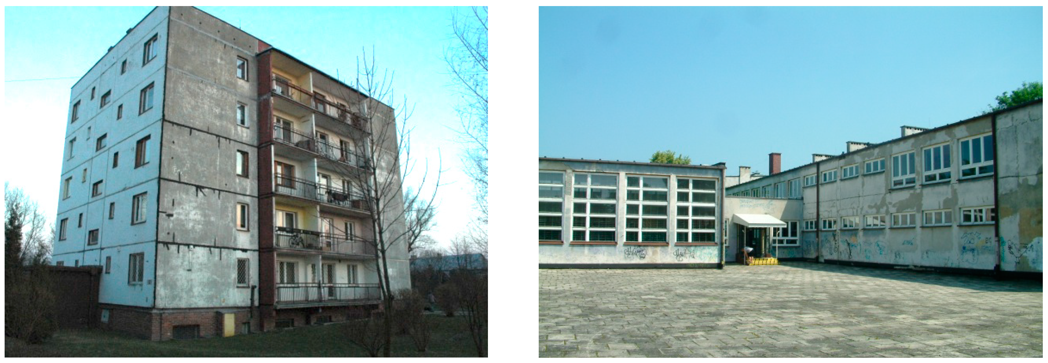
A multi-family freestanding residential five-story building with a basement was selected, made using large slab technology, put into operation in the mid-1980’s, see Figure 1. This building represents a typical multi-family building in Poland. The external walls are made of concrete and are insulated with mineral wool. The roof is ventilated, with a mineral wool insulating layer. Some of the windows in the building have been replaced with new ones, which meet the current requirements for insulation. The old and new windows differ in their sealing factor, see Table 1. On each floor, there are four flats (two with an area of 50.5 m2, one with an area of 60.5 m2, and one with an area of 73.5 m2). The heated building area is 1350 m2. The values of the heat transfer coefficients of each of the partitions have been summarized in Table 1. The building’s venting system is based on natural gravitational ventilation, executed through individual ventilation channels. The building is equipped with a central water heating system; the installation is powered by the municipal heating network. A total of 62 people reside in the building, according to the information about the residents.
The school building (primary school) selected for testing was built using pre-fabricated technology in the 1960s, see Figure 1. It is a two-story building without a basement, and the total heated area is 1406 m2. The building consists of two connected parts: A two-story main building, comprising of classrooms, office, toilets, kitchen, and cloakrooms, and a one-story gym building. All the windows and doors have been replaced with new ones (wooden or PVC windows)–the replacement work took place in several stages, so the windows are characterized by different airtightness factors, as shown in Table 1. The building is equipped with a gravity ventilation system and a water heating system with radiators. A solid fuel (coke) boiler is the source of heat. At weekends, the school is not heated. The school is used from Monday to Friday from 7 a.m. to 5 p.m. or 7 p.m. Classes are from 8 a.m. to 3 p.m. There are 137 students, 14 teachers, and 11 staff.
2.2. Models and Assumptions for the Simulation
Measurements of the energy consumption, internal temperature, and airtightness were carried out in both buildings, in order to get the input to the numerical models and carry out their validation. The time periods during February, March, and April were selected in to make the measurements. Such an approach allowed observation of both the cold and the transition periods of the heating season. An all-season measurement was not possible due to lack of access to flats (i.e., no consent from the buildings’ administrators for the long-term measurement).
Data loggers that ran on battery power were used to measure the temperature. The measurement range of the data loggers was −30 °C to 80 °C. The accuracy of the temperature measurement was ±0.5 °C in the range from 20 °C to 30 °C, and it could vary between 0.5–1.8 °C in the remaining range. The airtightness test was performed according to the ISO9972:2015 standard [23] and the fan pressure method used the Minneapolis Blower Door Model 4 (measuring range of air volume: 19–7200 m3/h with an uncertainty of ±4%; uncertainty of pressure difference measurement was ±1% of the reading’s value or 0.15 Pa). As a result of the measurements, the characteristics of airtightness of the test areas of the buildings that were recalculated from the infiltration coefficient were defined.
The internal temperature measurements in the residential building were studied in four selected flats; in two places on the staircase and in two places in the basement between February and April of 2011. In the prevailing period, the measured values of the dwelling’s temperature ranged from 20 °C to 24 °C. In the stairwell, there were values from 12 °C to 18.5 °C, and in the basement premises from 12 °C to 15.5 °C. In addition, energy consumption data were obtained for heating purposes throughout the heating season 2010/2011 (from October to early May): The heating power, delivered to the building for the purposes of the central heating system, was registered by the heat meter placed in the building. Airtightness tests were carried out in two flats with different types of windows (old/new).
In the school building, the temperature measurements were performed in February and March 2011 in ten rooms. In the school, the two-month period included two weeks of the winter holidays (1–13th of February). During the measuring period, data loggers recorded a temperature range of 10 to 25 °C. At the same time, the daily consumption of coke was also listed. Airtightness tests were conducted in two classrooms with different types of windows (PVC/wood).
During the measurements, the climatic data using the local weather station was recorded.
The analyses were performed by numerical simulation with the use of the integrated energy modeling tools TRNSYS [24] and ESP-r [25], which permitted integrated calculations of the transfer of mass and energy inside the buildings, taking into account the heating and air-conditioning systems, the sources of heat, and the control strategy. The buildings were described in the programs as macro-scale models, represented as a series of idealized zones with the constant parameters of the air within the limits of the entire zone. The models created in the programs possessed a well-imaged reality, which has been confirmed in many publications, including the authors of this article [26,27,28,29,30,31]. Due to the similar room properties (temperature, usage), some modifications have been made by combining several rooms into a single zone. This resulted in a residential building model that consisted of 26 zones and a model of the school building that consisted of five zones. The internal partitions were taken into account in the zones, which have an effect on the accumulation of heat. The construction of the walls and windows were modeled according to the actual state of the buildings.
The thermal models of the buildings included the following heat fluxes: Heat penetration through the external walls and roof, heat permeating through the internal partitions–walls, floors, resulting from solar radiation, transferred together with the air infiltration into the building, and emitted by the occupants, equipment, and lights. The output from the simulation was the heat demand for the entire building.
All of the simulation calculations were performed with a time step of 1 h. The ideal control for heating was assumed.
2.3. Models’ Validation and Calibration
The preliminary calculations were performed and the results of the simulation were compared with the results of the measurements. Validation was performed for the daily heat demand for the entirety of the buildings. The outdoor conditions were in accordance with the meteorological data from the local weather station. The model was then tuned to match the real object. In the subsequent tests, the following parameters were changed: Solar transmittance for windows, internal heat gains, and air infiltration (various airtightness factors for windows in accordance with the pressure tests).
2.3.1. The Residential Building
Validation was performed for the period from the 1st to the 28th of February. The calculations were based on the following assumptions:
- The indoor air temperature was adopted from the measurements. Flats zone–21.7 °C was used as a weighted average temperature in the flats; staircase and cellar–unheated, but additional heat gains were assumed from the heating and hot water pipes (which were poorly insulated) at the level of 8 W/m2.
- The air flow infiltrating into the zones–and the additional calculations of the ventilation air flows in the building were performed with the use of the CONTAM program [32]–the air change rate variable was in a 1-h time step. All the identified air flow paths, both the air infiltrating through the cracks in the windows and doors as well as the inter-zone air flows, were represented in the multi-zone numerical model that was built for the building; the air infiltration coefficients were determined from the airtightness measurements and the results were then imported into the TRNSYS program.
- To determine the internal heat gains, random surveys were carried out to verify the number of occupants, equipment, and the building use; constant heat gains were assumed in the simulations: 3.2–3.7 W/m2, depending on the type of flat.
- The efficiency of the heating system was assumed to be 0.83 based on the diagnosis of the heat source in the building and based on Polish law [33].
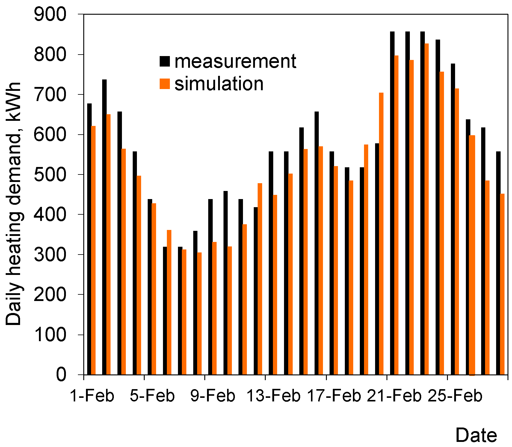
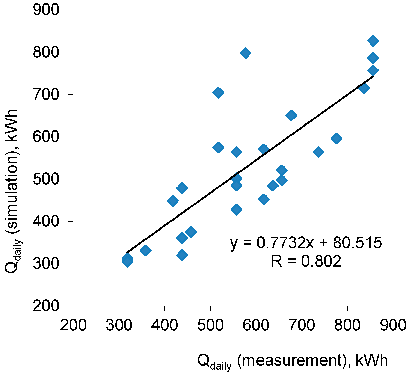
Figure 2 shows a comparison of the daily heat demand obtained from the measurements and simulation from February. The differences were from −22% to 30%. However, for a period of 20 days, the differences did not exceed the range of −15 to 15%. The correlation of the daily heat demand in the analyzed period has been shown in Figure 3. A good correlation was obtained, with a correlation coefficient R = 0.80.
2.3.2. The School Building
Validation was performed for the period from 14th February to 24th March. The holiday period was rejected because this period is characterized by atypical internal heat gains. The calculations were based on the following assumptions:
- The indoor air temperature in the zones in the heating season was adopted from the measurements (with a 1-h time step). The air temperature for the zones was determined as a weighted average of the measured temperature in particular rooms (the area was the weight).
- The air flow infiltrating into the zones–additional calculations of ventilation air flows in the building were performed with the use of the CONTAM program [32], similar to the residential building; the results were imported into the ESP-r program.
- A uniform heat gains schedule was adopted from Monday to Friday: Classes lasted from 8 a.m. to 3 p.m.; at the school there were 120 pupils, ten teachers, and eight service staff; after 1 p.m., the number of students at school decreased to 70; the number of lights was small, with a utilization factor of 0.2 to 0.4; outside of the lesson hours at the school, only the staff were present (up to 5 p.m.); computers were used from 8 a.m. to 3 p.m. in the computer rooms (utilization factor was 0.4). The school was not used on the weekends. Heat gains from lighting and the number of pieces of equipment were adopted in accordance with the building inventory. The amount of heat gain for one person and the heat gains from the equipment were adopted according to ASHRAE [34].
The real daily consumption of coke was converted into heat demand with the following assumptions: The caloric value of coke is 25 MJ/kg, the efficiency of the heating system was 0.55 according to Polish law [33]–taken as a constant, averaged for the entire validated period (based on the installation and boiler inspection).
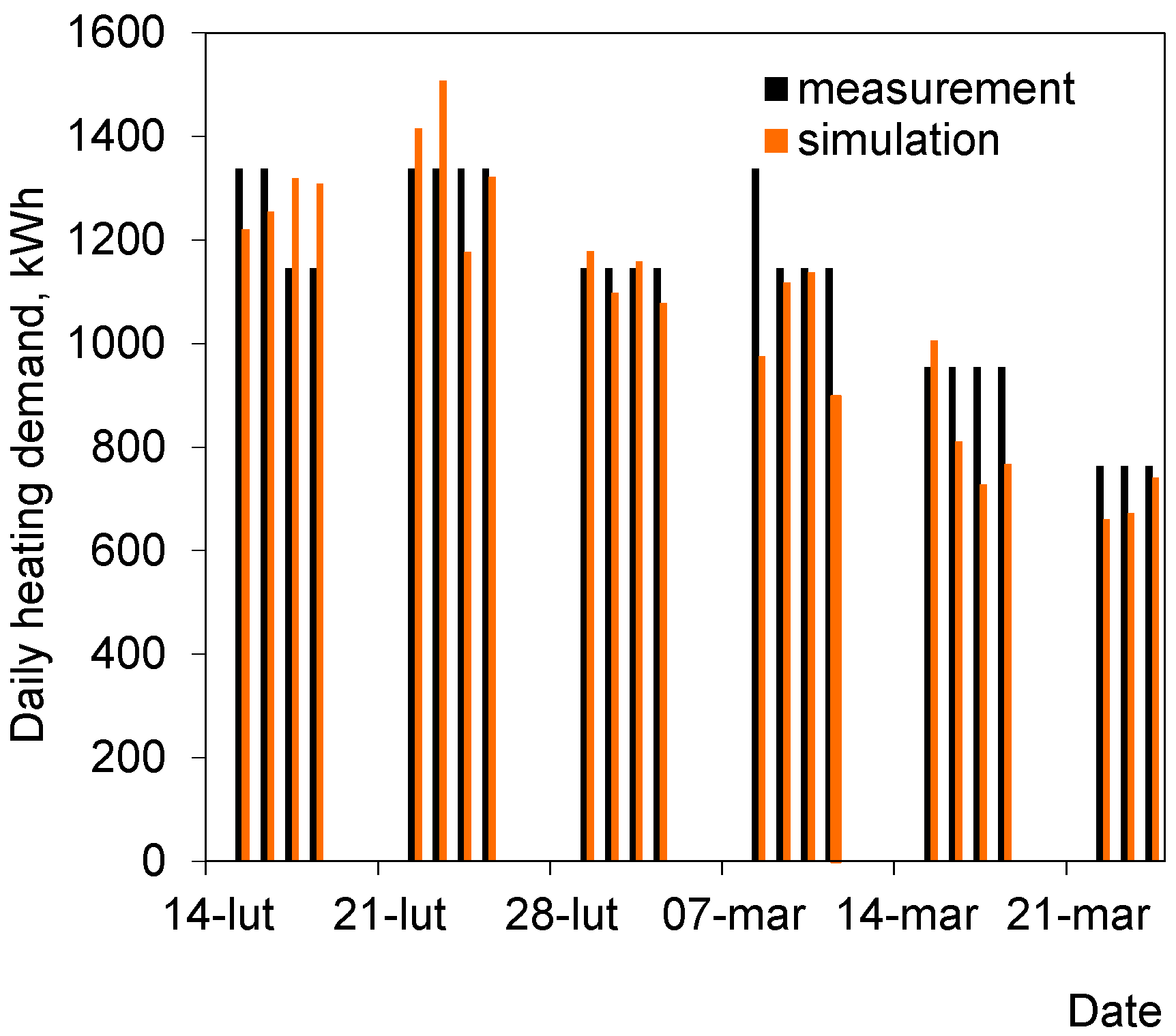
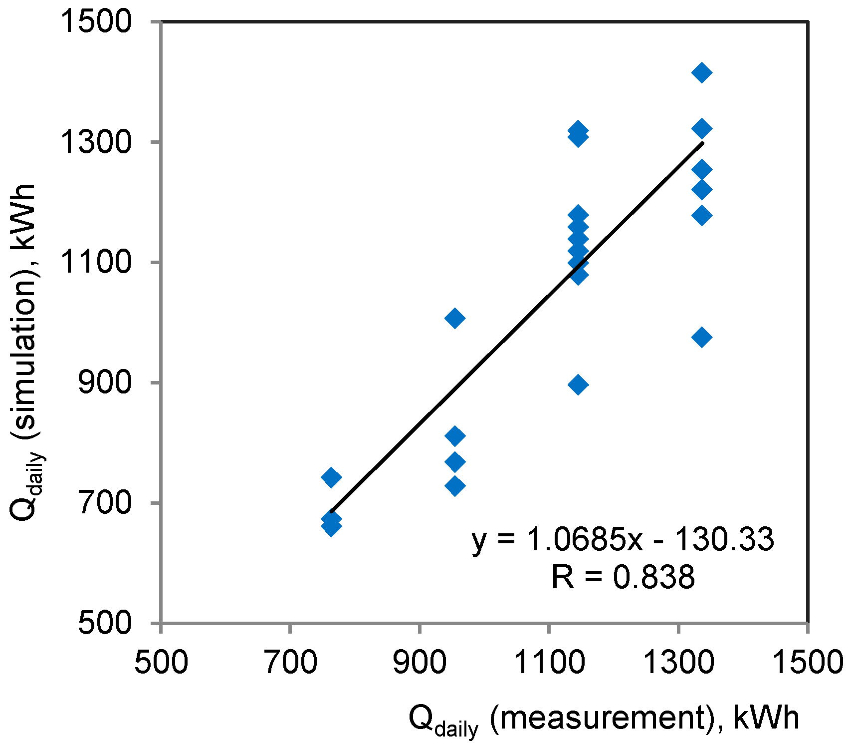
Figure 4 presents a comparison of the daily heat demand obtained from the measurements and simulation for the whole building. The differences ranged from −15% to 44%. The biggest differences were obtained on Mondays, after the boiler has been turned off over the weekend. The efficiency of the boiler on these days could have been significantly different from the assumed average. Excluding Mondays, the difference was within −15–27%, but for more than 60% of the time, the error did not exceed ± 10%. The correlation of the daily heat demand in the analyzed period, excluding Mondays, has been presented in Figure 5. A good correlation was obtained, and the correlation coefficient was R = 0.84.
These prepared (calibrated and validated) models then became the basis for further analyses. For the next all-season analyses, a schedule of the indoor temperature was introduced for each zone in the school model, with weekdays and weekends separated. The schedule was created on the basis of measurement data from February to March. The weighted average indoor temperature during class hours from 7 a.m. to 3 p.m. was 20 °C, and the rest of the time, including weekends, it was 19 °C and 16 °C.
2.4. Calculation Procedure
The energy signature method with linear regression was used to determine the energy consumption based on the empirical correlation with the outside temperature and then used to calculate the energy consumption during the heating or cooling season. This method assumed a constant internal temperature value, and the external air temperature was the parameter which affected the energy consumption the most. The analysis carried out in this study included the variability of the internal temperature value, which was to be taken into account as well as the internal heat gain. The method described in the EN 15603:2008 standard [5] was modified, making the heat demand conditional on the difference between the internal and external air temperature.
The purpose of the analysis was to draw up guidelines for the determination of the seasonal heat consumption for heating and ventilation during the heating season on the basis of short heat demand measurements. Simultaneously the optimum duration of the measuring period and estimation of the inaccuracy of the seasonal heat consumption, based on short measurements, was determined.
The analysis was performed for the averaged data on the individual days. Due to the thermal capacity of the building and the variability of the daily internal gains, there was no correlation between the power delivered to the heating and the thermal needs of the building at each hour–a time shift occurred.
Analyses were conducted for the heating season from October to April using typical Polish climatic data (Site Katowice [35]). The climate can be described as a temperate climate with relatively cold winters and warm summers.
Analyses were performed using the following steps:
- The hourly heat demand values of the building averaged to the mean daily value were calculated using computer simulation.
- The mean daily differences between the internal and external air temperature were calculated (timean-temean).
- The mean seasonal difference between the internal and external air temperature was calculated (dTmean,s).
- The seasonal demand for heat was calculated based on dependence–defined linear regressions in short time periods: Monthly, fortnightly, and weekly, moving the calculation period by one day starting from October 1st. Thus, there were 183 periods of 30 days, 199 periods of 14 days, and 206 periods of 7 days, each with a different value for the mean outside temperature. The analysis was performed using a Microsoft Excel worksheet by setting a value of the mean seasonal heat demand based on each short period. The values of the x-array were the differences between the mean values of the internal and external daily air temperature (timean-temean), and the values of the y-array was the mean daily heating power, Pmean. The mean seasonal difference between the internal and external temperature was assumed (dTmean,s) for the value for which the linear function value was calculated. Multiplying the value of the mean seasonal heating capacity for 24 h and the number of heating days (Lseason = 212 days), a seasonal heat demand was obtained on the basis of each short measuring period.
- The results from the periods for which the correlation coefficient R, between the power Pmean and the temperature difference (timean-temean), was less than 0.6 were rejected. The assumption of an accepted method for the energy signature is a good dependence of the measuring period of the power delivered to the building with the change in the outside temperature, or the difference between the internal and external temperature. According to the literature [36,37,38], a strong correlation is found when the correlation coefficient R is larger than 0.6–0.7.
- Calculated on the basis of a short period of seasonal value, the heat demand was compared to the value of the seasonal demand obtained through simulation. For each calculated period, the percentage differences (deviations), between the value of heat demand during the heating season (calculated by simulation) and the value of heat demand determined on the basis of the short period analyzed (measuring period), are stated.
The parameters used in the regression calculations are summarized in Table 2.
3. Results
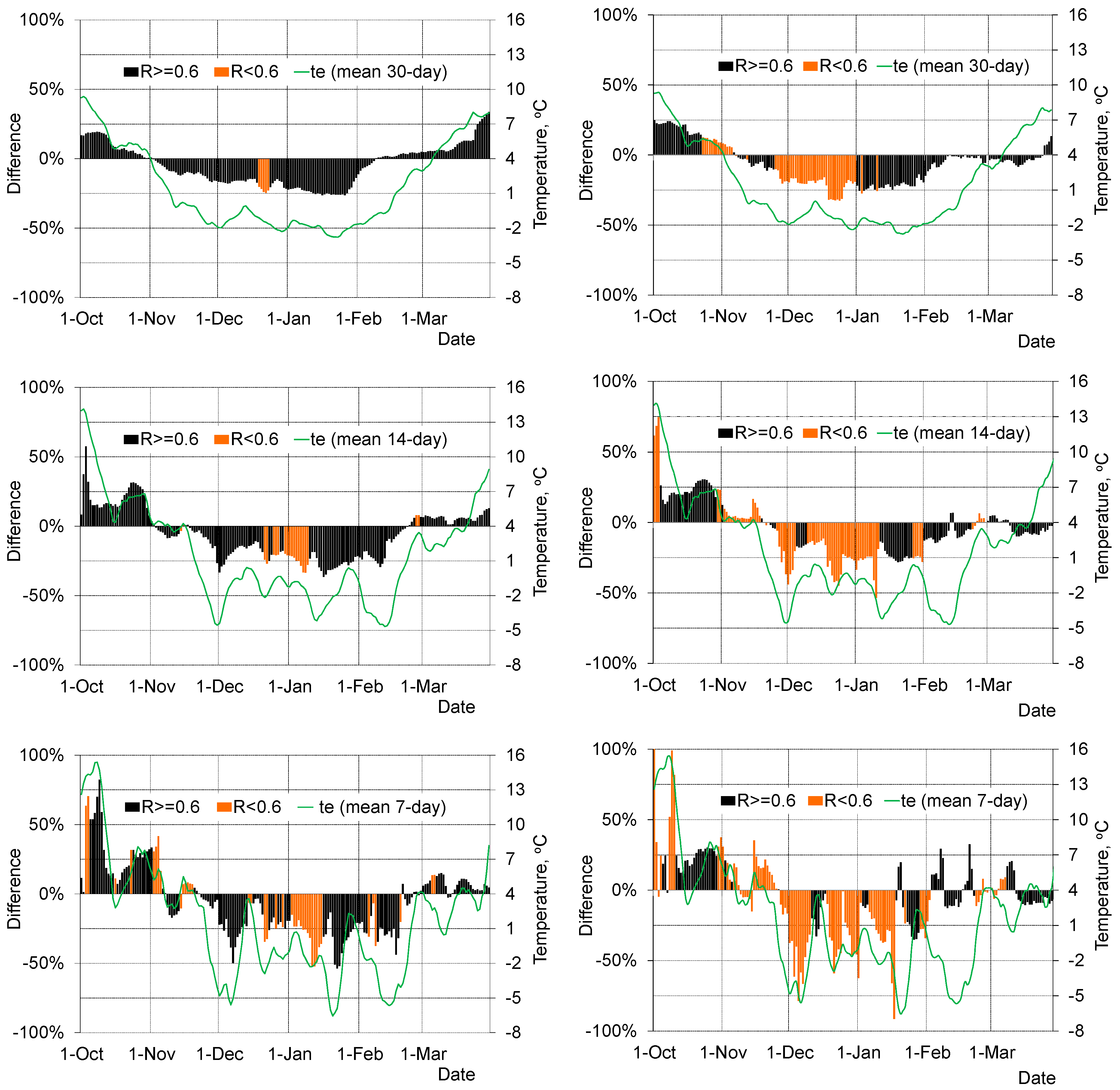
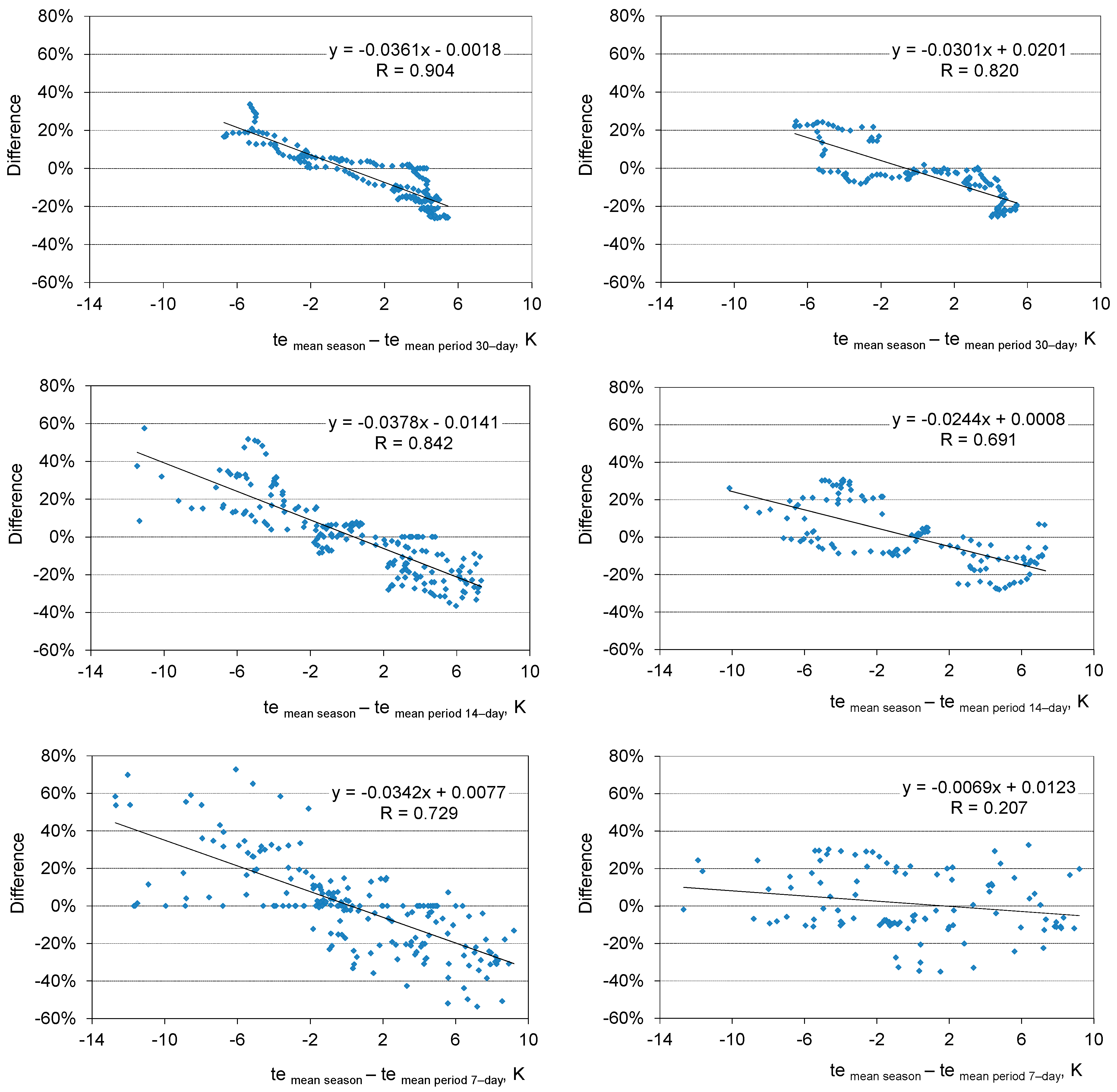
Table 3 presents the correlation of the mean daily heating power and the mean daily indoor and outdoor temperature difference for the whole heating season. Seasonal heat demand has also been presented. In both cases a strong correlation between heating power and the daily temperature difference was obtained: Residential building–0.93, school building–0.84. Seasonal heat demand, obtained by the regression method (according to the equations given in Table 3) for data from the whole season, was identical to that calculated in the simulation program. The results of the calculations based on the data from shorter periods were the worst. Figure 6 has shown the differences in the seasonal heat demand determined by mean daily heat demand from the 30-day, 14-day, and 7-day periods, in addition to the seasonal heat demand that was calculated by simulation. For periods in which the correlation coefficient was greater than 0.6, the correlation of the heat demand difference and the temperature difference (mean temperature: 2.66 °C and mean short period temperature: temean period) was evaluated, see Figure 7.
In the residential building, for the 30-day periods, only a few periods with a correlation coefficient of R < 0.6 were observed; there were five periods beginning on 19 December. There were 21 (11%) 14-day periods when the correlation coefficient was below 0.6, and in the case of the 7-day periods, it could be observed in 48 such periods (23%). The percentage differences in the seasonal heat demand determined in a short 30-day measurement range were from −30% to 30% (in relation to the seasonal heat demand from the simulation). For the 14-day periods, the differences were larger and ranged from −35% to 55% at temperature differences (temean season-temean period) in the range from 11 K to 7.5 K. The way in which it was possible to assume the heat demand values calculated from the seven-day periods were characterized by the largest differences from −60% to 80% at temperature differences from −13 K to 9 K.
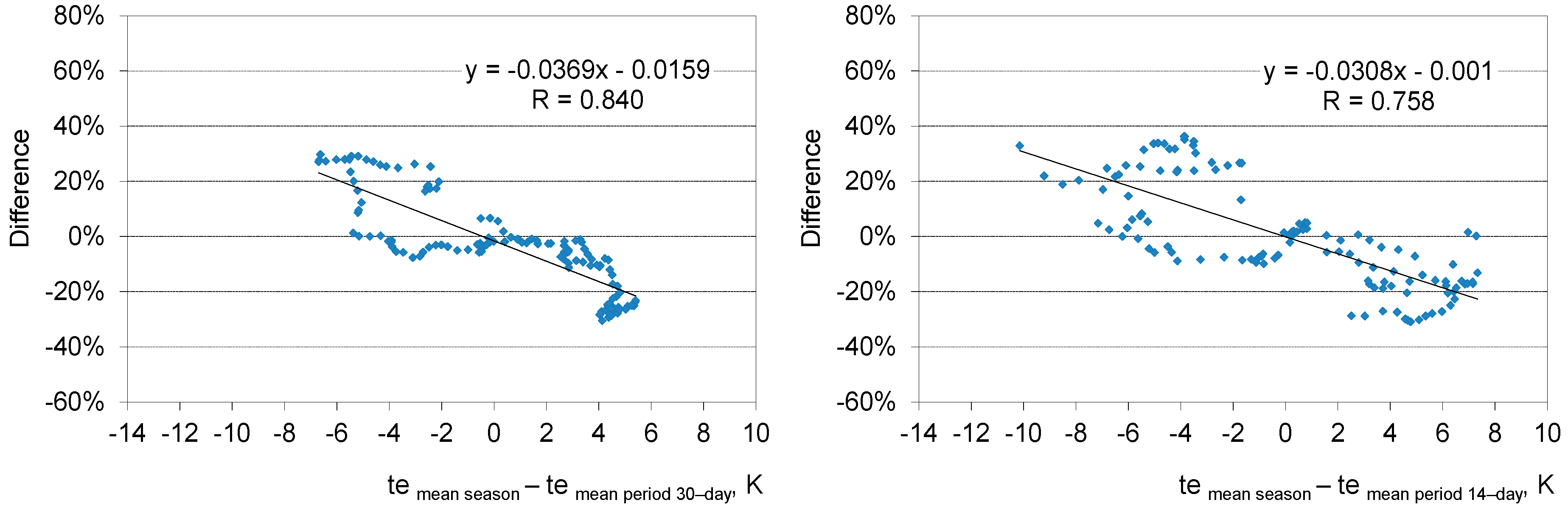
In the case of the school building, the 30-day periods with a correlation coefficient of R < 0.6 were as much as 55 (30%), and these were the periods between October and November and between the end of November and the beginning of January. There were 79 14-day periods for which the correlation coefficient was low, and these were mainly periods in November, December, and the first half of January. Among the seven-day measurement periods, the most periods with R < 0.6–103 (50%) should be rejected. For the rest of the periods (R > 0.6), for figures of the correlation of the seasonal heat demand percent differences and the temperature difference (the mean temperature of the heating season minus the mean temperature of the short period), it could be observed that: The percentage differences for the 30-day periods were −25% to 25% for temperatures differences in the range of −7 to 5 K; for the 14-day measurement periods the differences increased in relation to the calculation from the monthly periods and ranged from −28% to 30%, while for the seven-day periods they ranged from −35% to 33% at temperature differences from −13 K to 9 K.
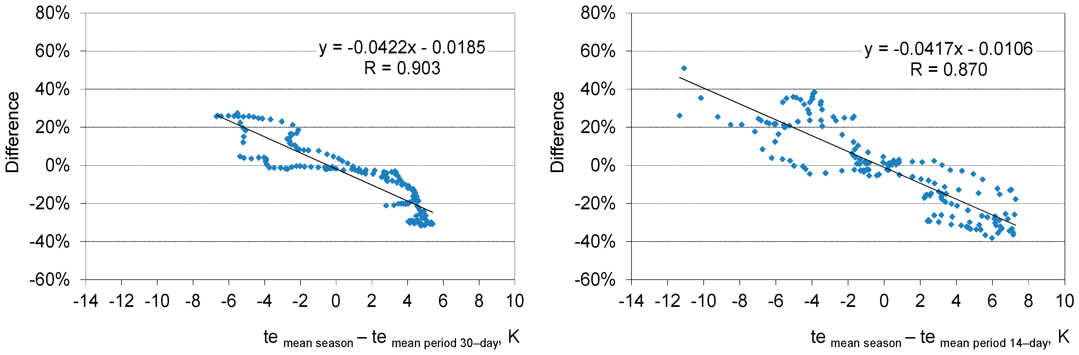
The shorter the measurement period, the weaker the correlation was between the errors obtained and the temperature difference (temean season-temean period). In the case of both buildings, the deviations did not exceed ±10% if the mean temperature of the 30-day short period did not differ by more than ±2.0 K from the mean temperature of the season. In turn, for the 14-day period, this temperature difference had to be in the range of −1.5 to 2.5 K.
In the next step, the influences of heat gains, ventilation intensity, and insulation of the building’s external partitions on the selection of the measurement period were checked. Because the analyses showed that the calculations based on the seven-day data were burdened with a large error, in the next analyses only the 30-day and the 14-day periods were considered.
3.1. The Less Airtight Building
The window’s airtightness factors were increased approximately twice. In the case of the residential building, for all windows, the airtightness factor was increased by up to 0.8 m3/mhPa0.67, and for the school building by up to 0.4 m3/mhPa0.67. In less airtight buildings, the heat demand for air infiltration increases. Therefore, the seasonal heat demand for the residential building increased to 508.6 GJ, and to 716.3 GJ for the school building.
Figure 8 shows the relationship between the percentage difference of seasonal heat demand and the temperature difference (the mean temperature of the heating season and the mean temperature of the short 30- or 14-day analyzed periods. In the case of the less airtight residential building (larger heat demand for ventilation), almost all short 30- and 14-day measurement periods were satisfactory for the calculation. Only in the case of five and six periods, respectively, was the correlation between the mean daily heat demand and the mean daily temperature difference (timean-temean) less than 0.6. However, it was noticed, that for the same range of temperature difference (temean season-temean period), the deviations in heat demand were a few percentage points higher for a less airtight building. Therefore, for the temperature difference from −4 K to 2.5 K, the differences in heat demand ranged from −10% to 12% for the 30-day periods and from −10% to 18% for the 14-day periods.
In the less airtight school, 41 (22%) monthly periods and 66 (33%) two-week periods were rejected (R < 0.6), i.e., lower by eight percentage points for monthly periods and seven percentage points for 14-day periods in comparison to the standard model. The ranges of the percentage differences in the seasonal heat demand determined from the short periods moved “down” by two percentage points for the 30-day periods and one percentage point for the 14-day periods. The differences for the monthly periods ranged from −27% (+2 points) to 23% (−2 points) at the same temperature differences (−7–5 K), and for the 14-day periods from −29% (+1 points) to 29% (−1 points) at the same temperature differences (−10–7 K) as in the case of the building with a higher airtightness.
For this building variant, the correlation between the heat demand difference and the temperature difference (temean season-temean period) was at a similar level as in the case of the more airtight building.
From the graphs, see Figure 8, it can be seen that the errors did not exceed ±10% if the difference between the mean temperature of the season and the mean temperature of a short 30-day period did not exceed the range of −2 to 4 K, and the 14-day period did not exceed the range of −1.5 to 2.5 K. This relation was observed both for the residential and the school building. As can be seen, the temperature difference range in which the deviation was ± 10% doubled in the case of the monthly periods. In the case of the 14-day periods, it remained the same as in the case of a more airtight building.
3.2. The Building with Well Insulated External Walls
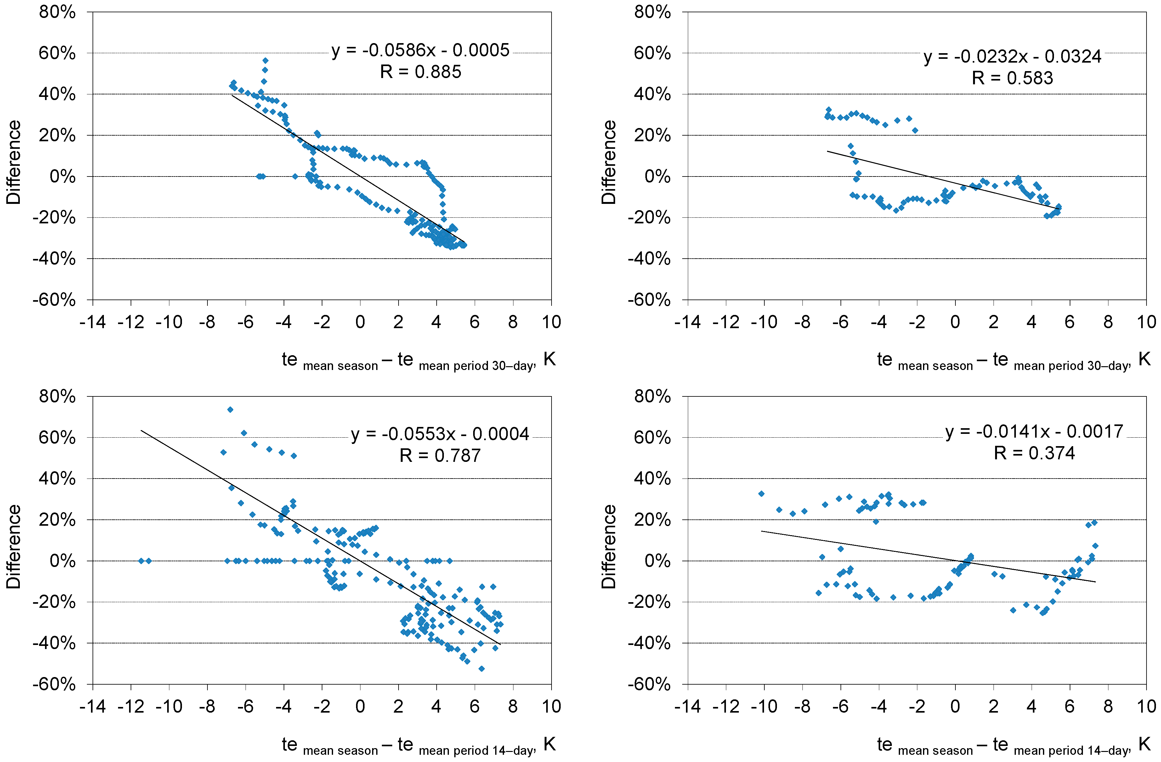
The external partitions of the buildings have been changed (additional insulating layers) so that the heat transfer coefficients were in accordance with the current Polish standards (Uwall = 0.30 W/m2K, Uroof = 0.25 W/m2K). In this case, the heat demand was less dependent on the external climate (less heat loss through the external partitions), and the total heat demand decreased in comparison to the standard buildings: Reduced to 209.8 GJ in the case of the residential building and to 432.4 GJ in the case of the school.
Figure 9 has shown the correlation between the percentage difference of the seasonal heat demand and the temperature difference between the mean temperature of the heating season and the mean temperature of the 30- or 14-day short period.
In the case of the well-insulated residential building, the heat demand differences over the whole season were in the range of −30% to 60% for the 30-day periods, the largest differences occurred during the transitional periods of the season. Therefore, for the temperature difference (temean season-temean period) from −4 K to 2.5 K the heat demand deviations were in the range from −20% to 20% for the 30-day periods and from −40% to 40% in the case of the 14-day periods.
It is also worth noting that the number of rejected periods (R < 0.6) was similar to the case of the less well-insulated building: Two and 25 periods were rejected for the 30-day and the 14-day periods, respectively.
In the case of the well-insulated school building, 115 (59%) of the monthly periods and 106 (53%) of the two-week periods were rejected (R < 0.6); much more than in the case of the standard building. The monthly periods, all from mid-October to mid-January were rejected. The 14-day periods, all from mid-October to mid-January and part of February and April were also rejected. For this variant, worse correlation coefficients between the heat demand difference and the temperature difference (temean season- temean period) were also obtained: For the monthly periods R = 0.58, and for the two-week periods R = 0.37. The ranges of the percentage differences in the seasonal heat demand, determined on the basis of these periods, moved upwards. The differences for the monthly periods ranged from −19% (−6 points) to 32% (+6 points) for the same temperature differences (7–5 K), and for the two-week periods from −25% (−3 points) to 33% (+3 points), the same as in the case of the less well insulated building, with the temperature difference (−10–7 K).
For the school building, the differences in heat demand did not exceed ±10% for the temperature difference (temean season-temean period) in the range 0–4 K for the monthly periods and in the range 0–3 K for the 14-day periods (with very poor correlation). In the case of the residential building, the differences in heat demand of ±10%, could only be obtained in the temperature difference range 0–0.5 K for both of the 30- and 14-day periods.
3.3. Usage of the Building
It can be seen that in the case of the public building, the number of rejected periods, with a weak correlation (R < 0.6) between the mean daily heat demand and the mean daily temperature difference (timean-temean), was higher than in the residential building. This may have been affected by the way the public building was used, i.e., only from Monday to Friday. To verify this thesis, additional calculations were made using the model of the school building, introducing the same usage schedule from Monday to Sunday.
It can be seen that the coefficients of the correlation between the heat demand differences and the temperature differences (temean season-temean period) significantly increased compared to the standard model, see Figure 10. In the analyzed case, only 13 monthly periods (7%, only in December) and 33 two-week periods (17%, mainly the end of December and at the beginning of January) were rejected (R < 0.6), which was significantly less than in the case of the standard use schedule.
In the case of the public buildings, due to the specificity of their use (only five days a week), the number of “good” measurement periods decreased. The relationship between the calculated heat demand from the short periods and the difference between the mean temperature of the heating season and the mean temperature of the short analyzed period also decreased, in comparison with buildings used all week in a similar way.
3.4. School Building with Large Internal Heat Gains
Internal heat gains in the model increased by an average of 55%. It was assumed that all pupils and teachers stayed at the school during the lesson hours. Outside of these hours, only the staff were in the school (until 7 p.m.). Lighting was used at a large level (utilization factor 0.5–0.8). The utilization factor for the computers was 0.7 between 8 a.m. and 3 p.m. in the computer rooms.
The large internal heat gains covered a significant part of the heat demand, which was why its seasonal value dropped to 571.7 GJ, compared to the standard building.
In the analyzed case of the building, 47 monthly periods and 78 two-week periods were rejected (R < 0.6), which was slightly less than in the case of the building with smaller heat gains. For this variant, the better coefficients of correlation meant that the daily heat demand and the mean daily temperature difference (timean-temean) were obtained, see Figure 11: R = 0.84 for the monthly periods, and R = 0.76 for the two-week periods. However, the obtained percentage differences in the seasonal heat demand determined on the basis of these periods were higher. The differences for the monthly periods increased “up” and “down” by an average of five percentage points and ranged from −31% to 30% at the same temperature differences (−7–5 K), and for the two-week periods from −31% (+3 points) to 36% (+6 points), which was the same for the case of the building with lower internal gains in the temperature differences (−10–7 K).
The differences in the heat demand did not exceed ± 10% for the calculations based on the monthly periods with a temperature difference of −2.0 to 2.5 K and for the 14-day periods with a temperature difference of −1.5–2.5 K. This was very much the same as for the building with smaller internal heat gains.
4. Conclusions
The following conclusions resulted from the conducted analyses regarding the calculation of the energy consumption for heating and ventilation based on short measurement periods using the energy signature method:
- The calculations that were based on the short measurement periods were burdened with the uncertainty of the estimation of the seasonal heat demand–presented as the difference between the seasonal heat demand and the seasonal heat demand determined from the short measurements; without an adjustment of the uncertainty value, the differences were ± 30% for the monthly measurement period, ± 40% for the two-week period, and ± 60% for the weekly period.
- A much smaller uncertainty could be obtained by rejecting the measurements for the transition periods of the heating season (October, March, and April).
- With the shortening of the measurement period, the correlation between the heat power and the difference in the internal and external daily temperature decreased, which necessitated the rejection of a significant number of the short periods; in the case of the public building, the number of “bad” seven-day measurement periods was as high as 50%;
- The number of “bad” measurement periods in the public buildings increased due to their specificity of use (only five days a week). For this reason, the errors in the calculated heat demand also increased compared to the buildings with the same internal heat gains during the whole week.
- The uncertainty in estimating the seasonal heat demand was, in most cases, strongly correlated with the difference between the mean temperature of the heating season and the mean temperature of the short period; as the temperature difference increased, the uncertainty of the estimation increased, and the uncertainty increased in the warmer periods of the season as well as when the measurement period was shortened.
- In public buildings, there was no correlation between the deviation of the calculated heat demand from the weekly periods and the difference between the mean temperature of the heating season and the mean temperature of the short periods; Therefore, measurements should be taken over longer periods.
- For the better-insulated building, the uncertainty of estimating the heat demand increased in relation to the building with less insulation on the external partitions; the number of “good” measurement periods was also reduced.
- For a more airtight building, the uncertainty of estimating the heat demand increased in relation to the building with less airtight windows.
- For the public buildings, an increase in the internal heat gains resulted in a small (around five percentage points) increase in the uncertainty of estimating the seasonal heat demand.
To sum up: The seven-day measurement period was insufficient to determine the seasonal heat demand, especially in public buildings that were not used during weekends.
The method presented requires modification by the introduction of correction factors. The results of preliminary analyses (that have not been presented in this article) carried out so far for two levels of thermal insulation in buildings and two types of climates have shown that the preparation of the correction factors will require a lot of work–carrying out a series of analyses for different climates and buildings; this work will be published in the future. The determination of the energy consumption for heating and ventilation will also be verified on the basis of the measurements.
Author Contributions
J.F.-G. and D.B. prepared and calibrated the simulation models, performed the simulations, and analyzed the results, A.S. contributed to the literature search and study design. The manuscript was improved and revised by K.G. All of the authors contributed to the paper writing.
Acknowledgments
The work was performed within the framework of research task No. 4: “The development of thermal diagnostics of buildings” within the Strategic Research Project funded by the National Center for Research and Development: “Integrated system for reducing energy consumption in the maintenance of buildings” and Statutory works BK-282/RIE1/2017, BK-249/RIE1/2018 and BK-207/RB-5/2018 funded by the Ministry of Science and Higher Education.
Conflicts of Interest
The authors declare no conflict of interest.
References
- EU Commission and Parliament. Directive 2010/31/EU of the European Parliament and the Council of the European Union of the 19 May 2010 on the Energy Performance of Buildings; Official Journal of the European Communities, European Parliament, the Council of the European Union: Brussels, Belgium, 2010; pp. 13–35. [Google Scholar]
- Afram, A.; Janabi-Sharifi, F. Review of modeling methods for HVAC systems. Appl. Therm. Eng. 2014, 67, 507–519. [Google Scholar] [CrossRef]
- Afram, A.; Janabi-Sharifi, F. Gray-box modeling and validation of residential HVAC system for control system design. Appl. Energy 2015, 137, 134–150. [Google Scholar] [CrossRef]
- Satyavada, H.; Baldi, S. An integrated control-oriented modelling for HVAC performance benchmarking. J. Build. Eng. 2016, 6, 262–273. [Google Scholar] [CrossRef] [Green Version]
- EU Standard EN 15603:2008 Energy Performance of Buildings—Overall Energy Use and Definition of Energy Ratings; European Committee for Standardization: Brussels, Belgium, 2008.
- Castillo, L.; Enriquez, R.; Jiménez, M.J.; Heras, M.R. Dynamic integrated method based on regression and averages, applied to estimate the thermal parameters of a room in an occupied office building in Madrid. Energy Build. 2014, 81, 337–362. [Google Scholar] [CrossRef]
- Belussi, L.; Danza, L. Method for the prediction of malfunctions of buildings through real energy consumption analysis: Holistic and multidisciplinary approach of Energy Signature. Energy Build. 2012, 55, 715–720. [Google Scholar] [CrossRef]
- Bartosz, D. The prediction of seasonal heat demand in residential buildings based on short-term calculations. Rynek Energii 2011, 96, 97–103. (In Polish) [Google Scholar]
- Freire, R.Z.; Oliveira, G.H.C.; Mendes, N. Development of regression equations for predictive energy and hygrothermal performance of buildings. Energy Build. 2008, 40, 810–820. [Google Scholar] [CrossRef]
- Ballarini, I.; Corrado, V. A new methodology for assessing the energy consumption of building stocks. Energies 2017, 10, 1102. [Google Scholar] [CrossRef]
- Sjogren, J.-U.; Andersson, S.; Olofsson, T. An approach to evaluate the energy performance of buildings based on incomplete monthly data. Energy Build. 2007, 39, 945–953. [Google Scholar] [CrossRef]
- Sjogren, J.-U.; Andersson, S.; Olofsson, T. Sensitivity of the total heat loss coefficient determined by the energy signature approach to different time periods and gained energy. Energy Build. 2009, 41, 801–808. [Google Scholar] [CrossRef]
- Vesterberg, J.; Andersson, S.; Olofsson, T. Robustness of a regression approach, aimed for calibration of whole building energy simulation tools. Energy Build. 2014, 81, 430–434. [Google Scholar] [CrossRef]
- Vesterberg, J.; Andersson, S.; Olofsson, T. A single-variate building energy signature approach for periods with substantial solar gain. Energy Build. 2016, 122, 185–191. [Google Scholar] [CrossRef]
- Catalina, T.; Iordache, V.; Caracaleanu, B. Multiple regression model for fast prediction of the heating energy demand. Energy Build. 2013, 57, 302–312. [Google Scholar] [CrossRef]
- Lam, J.C.; Wan, K.K.W.; Liu, D.; Tsang, C.L. Multiple regression models for energy use in air-conditioned office buildings in different climates. Energy Convers. Manag. 2010, 51, 2692–2697. [Google Scholar] [CrossRef]
- Amiri, S.S.; Mottahedi, M.; Asadi, S. Using multiple regression analysis to develop energy consumption indicators for commercial buildings in the U.S. Energy Build. 2015, 109, 209–216. [Google Scholar] [CrossRef]
- Asadi, S.; Amiri, S.S.; Mottahedi, M. On the development of multi-linear regression analysis to assess energy consumption in the early stages of building design. Energy Build. 2014, 85, 246–255. [Google Scholar] [CrossRef]
- Catalina, T.; Virgin, J.; Blanco, E. Development and validation of regression models to predict monthly heating demand for residential buildings. Energy Build. 2008, 40, 1825–1832. [Google Scholar] [CrossRef]
- Aranda, A.; Ferreira, G.; Mainar-Toledo, M.D.; Scarpellini, S.; Sastresa, E.L. Multiple regression models to predict the annual energy consumption in the Spanish banking sector. Energy Build. 2012, 49, 380–387. [Google Scholar] [CrossRef]
- Braun, M.R.; Altan, H.; Beck, S.B.M. Using regression analysis to predict the future energy consumption of a supermarket in the UK. Appl. Energy 2014, 130, 305–313. [Google Scholar] [CrossRef]
- Dong, B.; Lee, S.E.; Sapar, M.H. A holistic utility bill analysis method for baselining whole commercial building energy consumption in Singapore. Energy Build. 2005, 37, 167–174. [Google Scholar] [CrossRef]
- ISO Standard ISO 9972:2015 Thermal Performance of Buildings–Determination of Air Permeability of Buildings–Fan Pressurization Method; International Organization for Standardization: Geneva, Switzerland, 2015.
- Klein, S.A.; Beckman, W.A.; Mitchell, J.W.; Duffie, J.A.; Duffie, N.A.; Freeman, T.L.; Mitchell, J.C.; et al. TRNSYS 17 A Transient System Simulation Program; U. of W.-M. Solar Energy Laboratory: Madison, WI, USA, 2010. [Google Scholar]
- University of Strathclyde Energy Systems Research Unit. The ESP-r System for Building Energy Simulation; User Guide Version 10 Series; ESRU Manual U02/1; University of Strathclyde Energy Systems Research Unit: Glasgow, UK, 2002. [Google Scholar]
- Strachan, P.A.; Kokogiannakis, G.; Macdonald, I.A. History and development of validation with the ESP-r simulation program. Build. Environ. 2008, 43, 601–609. [Google Scholar] [CrossRef] [Green Version]
- Baranowski, A.; Ferdyn-Grygierek, J. Heat demand and air exchange in a multifamily building–simulation with elements of validation. Build. Serv. Eng. Res. Technol. 2009, 30, 227–240. [Google Scholar] [CrossRef]
- Judkoff, R.; Balcomb, J.D.; Subbarao, K.; Hancock, C.E.; Barker, G. Side-by-Side Thermal Tests of Modular Offices: A Validation Study of the STEM Method; NREL Technical Report NREL/TP-550-23940; National Renewable Energy Laboratory: Golden, CO, USA, 2000.
- Judkoff, R.; Balcomb, J.D.; Subbarao, K.; Hancock, C.E.; Barker, G. Barker, Building in a Test Tube: Validation of the STEM Method; NREL Technical Report NREL/TP-550-29805; National Renewable Energy Laboratory: Golden, CO, USA, 2001.
- Calise, F.; Figaj, R.D.; Vanoli, L. Energy and economic analysis of energy savings measures in a swimming pool centre by means of dynamic simulations. Energies 2018, 11, 2182. [Google Scholar] [CrossRef]
- Ogando, A.; Cid, N.; Fernández, M. Energy modelling and automated calibrations of ancient building simulations: A case study of a school in the northwest of Spain. Energies 2017, 10, 807. [Google Scholar] [CrossRef]
- Walton, W.G.N.; Dols, S. CONTAM 2.4 User Guide and Program Documentation; National Institute of Standards and Technology: Gaithersburg, MD, USA, 2005.
- Polish Ministry of Infrastructure. Regulation of the Minister of Infrastructure of 27 February 2015 on the Methodology for Calculating the Energy Performance of a Building or Part of a Building and Energy Performance Certificates; Journal of Laws of the Republic of Poland, Item. 376; Polish Ministry of Infrastructure: Warsaw, Poland, 2015. (In Polish)
- American Society of Heating, Refrigerating and Air Conditioning Engineers. ASHRAE Handbook, Fundamentals, SI ed.; American Society of Heating, Refrigerating and Air Conditioning Engineers: Atlanta, GA, USA, 1997. [Google Scholar]
- Typical Meteorological and Statistical Climatic Data for Energy Calculations of Buildings. Available online: https://www.miir.gov.pl/strony/zadania/budownictwo/charakterystyka-energetyczna-budynkow/dane-do-obliczen-energetycznych-budynkow-1/ (accessed on 1 June 2018).
- Jackson, S.L. Research Methods, A Modular Approach; Thomson Wadsworth: Belmond, CA, USA, 2008. [Google Scholar]
- Evans, J.D. Straightforward Statistics for the Behavioral Sciences; Brooks/Cole Publishing: Pacific Grove, CA, USA, 1996. [Google Scholar]
- Wang, M.; Wright, J.; Brownlee, A.; Buswell, R. A comparison of approaches to stepwise regression on variables sensitivities in building simulation and analysis. Energy Build. 2016, 127, 313–326. [Google Scholar] [CrossRef] [Green Version]
Figure 1.
Views of the buildings that were chosen to be researched: A multifamily residential building (on the left) and a school building (on the right).
Figure 1.
Views of the buildings that were chosen to be researched: A multifamily residential building (on the left) and a school building (on the right).

Figure 2.
Measured and simulated daily heat demand in the residential building.

Figure 3.
Correlation of the measured and simulated daily heat demand in the validated period for the residential building.
Figure 3.
Correlation of the measured and simulated daily heat demand in the validated period for the residential building.

Figure 4.
Measured and simulated daily heat demand in the school building.

Figure 5.
Correlation of measured and calculated daily heat demand in the validated period (excluding Mondays) for the school building.
Figure 5.
Correlation of measured and calculated daily heat demand in the validated period (excluding Mondays) for the school building.

Figure 6.
Differences in seasonal heat demand obtained from simulation and from short measurement periods for the residential building (on the left) and for the school building (on the right).
Figure 6.
Differences in seasonal heat demand obtained from simulation and from short measurement periods for the residential building (on the left) and for the school building (on the right).

Figure 7.
Correlation between the seasonal heat demand difference and external temperature difference (mean for the season and mean for each short period) for the residential building (on the left) and for the school building (on the right); only for periods with R ≥ 0.6, see Figure 6.
Figure 7.
Correlation between the seasonal heat demand difference and external temperature difference (mean for the season and mean for each short period) for the residential building (on the left) and for the school building (on the right); only for periods with R ≥ 0.6, see Figure 6.

Figure 8.
Correlation between the seasonal heat demand difference and external temperature difference (mean for the season and mean for each short period) for the less airtight residential building (on the left) and for the less airtight school building (on the right); only for periods with R ≥ 0.6.

Figure 9.
Correlation between the seasonal heat demand difference and external temperature difference (mean for the season and mean for each short period) for the better insulated residential building (on the left) and for the better insulated school building (on the right); only for periods with R ≥ 0.6.

Figure 10.
Correlation between seasonal heat demand difference in the school building, used all week, and the external temperature difference (mean for the season and mean for each short period) for the 30-day measured periods (on the left) and for the 14-day measured periods (on the right); only for periods with R ≥ 0.6.

Figure 11.
Correlation between the seasonal heat demand difference in the school building with large internal heat gains and the external temperature difference (mean for the season and mean for each short period) for the 30-day measured periods (on the left) and for the 14-day measured periods (on the right); only for periods with R ≥ 0.6.


Table 1.
Values of heat transfer coefficient of partitions in the studied buildings, including aging effects and thermal bridges.
Table 1.
Values of heat transfer coefficient of partitions in the studied buildings, including aging effects and thermal bridges.
| Partition | Heat Transfer Coefficient U, W/m2K | |
|---|---|---|
| Residential Building | School Building | |
| External wall | 0.62 | 1.27 |
| Roof | 0.41 | 0.69 |
| Floor to unheated cellar | 1.50 | - |
| Ground floor | 1.90 | 0.92 |
| Windows | 1.5 */2.6 ** | 1.5 |
| Airtightness factor for windows a, m3/mhPa0.67 | ||
| 0.20 *; 0.45 ** | 0.24; 0.21 | |
* new windows (PVC). ** old windows (wooden).
Table 2.
Parameters used in the regression calculations.
| Parameter | Symbol | Unit |
|---|---|---|
| Mean daily indoor and outdoor temperature difference | (timean-temean) | K |
| Mean daily heating power | Pmean | kW |
| Mean seasonal indoor and outdoor temperature difference | dTmean,s | K |
| Length of the heating season | 24 × Lseason | h |
Table 3.
Seasonal results and correlation of mean daily heat demand and mean daily internal and external temperature difference for the residential building (on the left) and school building (on the right).
Table 3.
Seasonal results and correlation of mean daily heat demand and mean daily internal and external temperature difference for the residential building (on the left) and school building (on the right).
| Residential Building | School Building | ||
|---|---|---|---|
| temean,s | 2.66 °C | temean,s | 2.66 °C |
| dTmean,s | 19.04 °C | dTmean,s | 15.96 °C |
| Pmean,s | 16.95 kW | Pmean,s | 34.4 kW |
| Qseason | 310.5 GJ | Qseason | 630.3 GJ |
 |  | ||
© 2018 by the authors. Licensee MDPI, Basel, Switzerland. This article is an open access article distributed under the terms and conditions of the Creative Commons Attribution (CC BY) license (http://creativecommons.org/licenses/by/4.0/).
Share and Cite
MDPI and ACS Style
Ferdyn-Grygierek, J.; Bartosz, D.; Specjał, A.; Grygierek, K. Analysis of Accuracy Determination of the Seasonal Heat Demand in Buildings Based on Short Measurement Periods. Energies 2018, 11, 2734. https://doi.org/10.3390/en11102734
AMA Style
Ferdyn-Grygierek J, Bartosz D, Specjał A, Grygierek K. Analysis of Accuracy Determination of the Seasonal Heat Demand in Buildings Based on Short Measurement Periods. Energies. 2018; 11(10):2734. https://doi.org/10.3390/en11102734
Chicago/Turabian StyleFerdyn-Grygierek, Joanna, Dorota Bartosz, Aleksandra Specjał, and Krzysztof Grygierek. 2018. "Analysis of Accuracy Determination of the Seasonal Heat Demand in Buildings Based on Short Measurement Periods" Energies 11, no. 10: 2734. https://doi.org/10.3390/en11102734
Note that from the first issue of 2016, this journal uses article numbers instead of page numbers. See further details here.