A Hybrid Ant Colony and Cuckoo Search Algorithm for Route Optimization of Heating Engineering
by
 , , ,
, , ,
Yang Zhang
1,2 ,
,
Huihui Zhao
2,
Yuming Cao
1,*,
Qinhuo Liu
2,* ,
,
Zhanfeng Shen
2,
Jian Wang
3 and
Minggang Hu
1 1
North China Power Engineering Co., Ltd. of China Power Engineering Consulting Group, Beijing 100120, China
2
State Key Laboratory of Remote Sensing Science, Institute of Remote Sensing and Digital Earth, Chinese Academy of Sciences, Beijing 100101, China
3
School of Geomatics and Urban Spatial Informatics, Beijing University of Civil Engineering and Architecture, Beijing 100044, China
*
Authors to whom correspondence should be addressed.
Energies 2018, 11(10), 2675; https://doi.org/10.3390/en11102675
Submission received: 19 September 2018
/
Revised: 27 September 2018
/
Accepted: 3 October 2018
/
Published: 8 October 2018
Abstract
:The development of remote sensing and intelligent algorithms create an opportunity to include ad hoc technology in the heating route design area. In this paper, classification maps and heating route planning regulations are introduced to create the fitness function. Modifications of ant colony optimization and the cuckoo search algorithm, as well as a hybridization of the two algorithms, are proposed to solve the specific Zhuozhou–Fangshan heating route design. Compared to the fitness function value of the manual route (234.300), the best route selected by modified ant colony optimization (ACO) was 232.343, and the elapsed time for one solution was approximately 1.93 ms. Meanwhile, the best route selected by modified Cuckoo Search (CS) was 244.247, and the elapsed time for one solution was approximately 0.794 ms. The modified ant colony optimization algorithm can find the route with smaller fitness function value, while the modified cuckoo search algorithm can find the route overlapped to the manual selected route better. The modified cuckoo search algorithm runs more quickly but easily sticks into the premature convergence. Additionally, the best route selected by the hybrid ant colony and cuckoo search algorithm is the same as the modified ant colony optimization algorithm (232.343), but with higher efficiency and better stability.
1. Introduction
With the acceleration of urbanization, heating engineering has become a common municipal infrastructure in modern cities, especially in the northern part of China. Central-heating facilities can significantly amplify the scale effect and protect the environment. Because the heating route often crosses the city and the engineering is mainly carried out underground, the heat routing decision-making process becomes more complicated. The job has been based on manual design until now.
The travelling salesman problem (TSP) is a kind of route optimization problem where a salesperson has to visit a list of cities exactly once and then return to the departure city, with the aim of minimizing the total travelled distance or the overall cost of the trip [1]. Regarding the heating engineering route selection problem, there are several similarities compared with the TSP. For example, the visited cities should also be passed only once, and the aim is also to find the minimum of the fitness function. However, the optimum heating route does not traverse all cities, and the specific start point and end point of the route are usually different; furthermore, the route must follow several regulations rather than be selected randomly. Therefore, we referenced the intelligent algorithms suitable for the TSP and devoted them to improving and proposing an effective algorithm to settle our heating engineering route selection problem.
Generally, intelligent algorithms can be classified into three types [2]: evolutionary algorithms (EAs) [3,4], trajectory-based algorithms [5,6], and swarm-intelligence (SI)-based algorithms [7,8]. SI-based algorithms often inspired by nature, especially biological systems. Through mimicking a population of simple agents or boids, the noncentralized control individual act should lead to the emergence of “intelligent” global behavior. SI-based algorithms can select the optimum solution by iterations of a number of generations. At each generation, the solutions are normally constructed based on historical information gained from previous generations [9]. Examples of SI-based algorithms include ant colony optimization (ACO) [10], particle swarm optimization (PSO) [11], artificial bee colony (ABC) [12], firefly algorithm (FA) [13], cuckoo search approach(CSA) [14], and intelligent water drops (IWD) [15]. There have been several research achievements using SI-based algorithms to address the TSP. In this study, we chose ACO and CSA as our research object, as both of them are well developed, high-performance algorithms that complement each other well.
ACO was developed by Dorigo in 1991 inspired by the behavior of ants seeking for food [10]. In the natural world, ants of some species (initially) wander randomly, and upon finding food return to their colony while laying down pheromone trails. The other ants are more likely to follow the trail with higher pheromones and release their own pheromones along their trails. Meanwhile, the pheromone trail evaporates over time, thus reducing its attractive strength. The more time it takes for an ant to travel down the path and back again, the more time the pheromones have to evaporate. That is, the pheromone between two nodes may be reinforced and evaporated simultaneously. The positive feedback eventually leads to many ants following a single path, and the optimum path is selected.
ACO was originally used for discrete optimization problems, and it specializes in solving the TSP. Although ACO was proposed a relatively long time ago, it is still widely used. Various studies have developed and improved the algorithm, such as the elitist ant system [16,17], the rank-based ant system (ASrank) [18], the max–min ant system (MMAS) [19,20], and the ant colony system (ACS) [21]. All of them are based on the modification of the ACO algorithm by adjusting the parameters or changing the search strategy. Most of the extension algorithms have been tested on the TSP, which confirms the central role of this problem in ACO research. There have also been some improvements to the parameters in recent years. Yu et al. [22] proposed ACO with a new “ant-weight strategy” pheromone updating rule; based on experimental results, they found that the proposed algorithm was effective for the capacitated vehicle routing problem (CVRP), which was a generalized TSP. Tuba et al. [23] proposed a new type of ACO and implemented it for the TSP. The method was based on pheromone trail correction and can avoid search stagnation. The correction calculation was based on the properties of the best-found solution so far. Meanwhile, there are some studies devoted to hybrid ACO with other intelligent algorithms to increase efficiency. Chen and Chien presented the genetically simulated annealing ant colony system with PSO techniques for solving the TSP [24]. Deng et al. [25] proposed a novel two-stage hybrid algorithm called the GA-PSO-ACO algorithm that combined the evolutionary ideas of the genetic algorithms, PSO and ACO. Mahi [26] proposed a new hybrid method to optimize parameters using PSO. In addition, the 3-opt heuristic method was added to the proposed method to improve local solutions. Zhang coupled ACO with path relinking method to solve the TSP [27]. Kaabachi implied the decision support system to highlight the performance of ACO [28]. Wei introduced the minimum spanning tree and proposed an evolutionary ACO algorithm [29].
CSA was developed by Yang and Deb [14] in 2009 inspired by the brood parasitism behavior of cuckoos. Cuckoos lay eggs in the host’s nest by Lévy flights and carefully matches its eggs to the host’s eggs. If the host recognizes the cuckoo’s eggs in its nest, it will either throw the eggs out or simply desert its nest and make a new one elsewhere. The surviving eggs hatch and the birds grow up, and the cycle of the next generation starts. The best nest is selected after a number of generations have been produced. CSA is a relatively new algorithm that has rapidly developed since it was proposed. It is effective in solving continuous optimization problems [30,31]. However, there have also been several attempts to modify and apply the algorithm to the discrete TSP. Generally, the modification can be categorized into two classes. One is the adjustment of the parameters, and the other is hybridization with other intelligence algorithms [32]. For the first method, Uroš Mlakar et al. [33] proposed a hybrid self-adaptive CS algorithm (HSA-CS) with which the search space was explored using three exploration search strategies, i.e., random long-distance search strategy, stochastic moderate-distance search strategy and stochastic short-distance search strategy. Saelim et al. [34] proposed crossover and random replacement for generating new solutions in place of Lévy flight, and the switching parameter pa was treated as being adaptive. The proposed algorithm was used to solve seven TSPs, and outperformed the original CS. Ouaarab et al. [35] proposed the random-key cuckoo search (RKCS) algorithm for solving the TSP. RKCS can switch between the continuous and combinatorial search space, which enable cuckoo search to provide a good search mechanism with a fine balance between intensification and diversification. Additionally, Ouaarab et al. [36] improved and developed the CSA by rebuilding three types of cuckoos. The new category of the cuckoo made it possible to perform more efficiently with fewer iterations. For the second method, Abu-Srhan et al. [37] combined CS with GA to avoid the local minima problem and to benefit from the advantages of both types of algorithms. A 2-opt operation was added to the algorithm to improve the results. Teymourian et al. [38] enhanced the IWD and CS algorithms for solving the CVRP. The authors approached the CVRP with four state-of-the-art algorithms: an improved intelligent water drops (IIWD) algorithm; an advanced cuckoo search (ACS) algorithm; and two hybrid algorithms coupling these methods, called a local search hybrid algorithm (LSHA) and a post-optimization hybrid algorithm (POHA). LSHA and POHA took advantage of the merits of ACS and IIWD, and can effectively handle CVRP, where in most cases, LSHA outperformed other three algorithms in the literature. Besides, CS has been hybrided with improved shuffled frog leaping algorithm [39], global harmony search algorithm [40], simulated annealing algorithm [41], FA [42] and so on.
As mentioned above, there have been various studies on ACO and CS aimed at solving the TSP. However, studies for optimizing the heating route in reality are rare. The ACO algorithm is constructive to global search, whereas the CS algorithm is capable to localized search. Therefore, a hybrid algorithm that combines the two ideas may result in a two-stage procedure that can surpass each of them individually. In this paper, we modified the ACO and CS algorithms, and proposed a hybrid ant colony and cuckoo search (HACCS) algorithm to combine the advantages of both algorithms. The HACCS was then applied to the Zhuozhou–Fangshan (ZF) heating engineering project.
This study is organized as follows. Section 2 introduces the study area and the study context, and the principle of heating route selection is provided as well. Data organization and management methods are supplied for subsequent applications. Section 3 provides the fundamentals and improvements of ACO and CSA algorithms, as well as the hybrid HACCS algorithm. Section 4 shows the operation results of the modified ACO, the modified CS and the HACCS algorithms. The results are compared with the real route that was selected manually. Finally, Section 5 discusses the findings and draws the concluding remarks. Several future research directions of interest are outlined.
2. Materials and Methods
2.1. Study Area
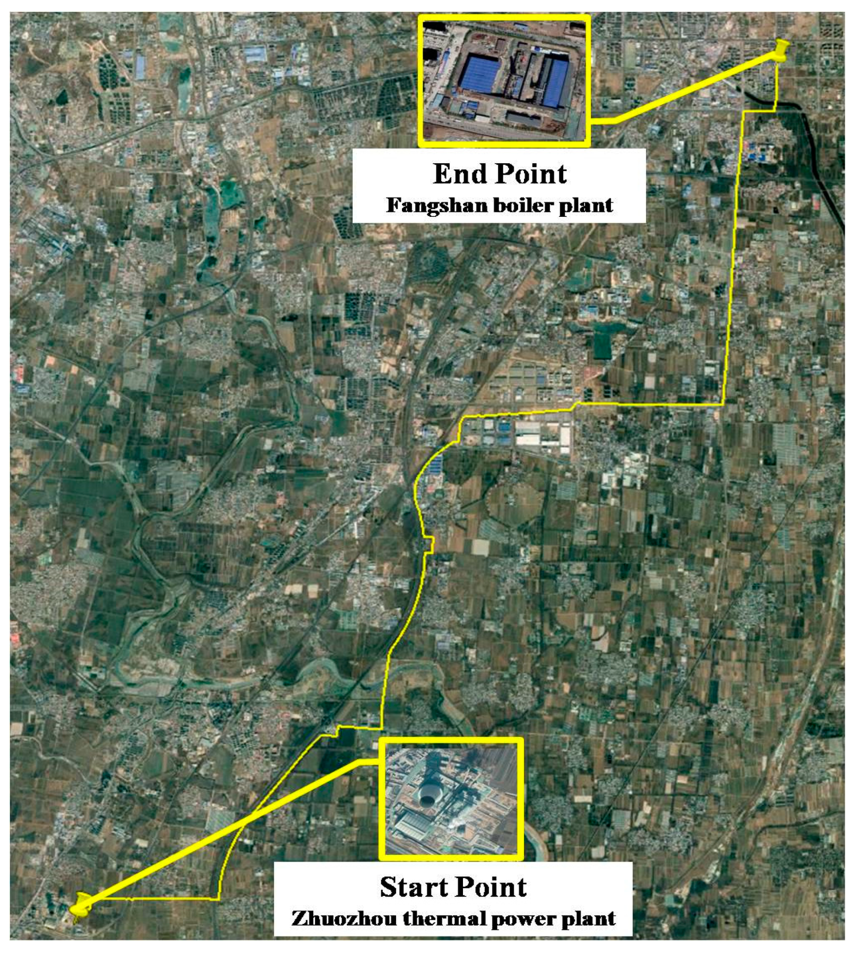
The ZF heating engineering project is important according to the 13th five-year plan for China energy development. The project is beneficial to Jing-Jin-Ji collaborative development and can significantly optimize the energy structure of Beijing. The total heating coverage of the project is approximately 35 million square meters. After the implementation of the project, the coal consumption of heating, CO2 emissions, carbon emissions, SO2 emissions, and NOx emissions can be reduced by 425,000 tons, 623,000 tons, 17 tons, 34 tons, and 102 tons per year, respectively. Thus, it plays an important role in the improvement of the regional urban environment and the residents’ quality of life.
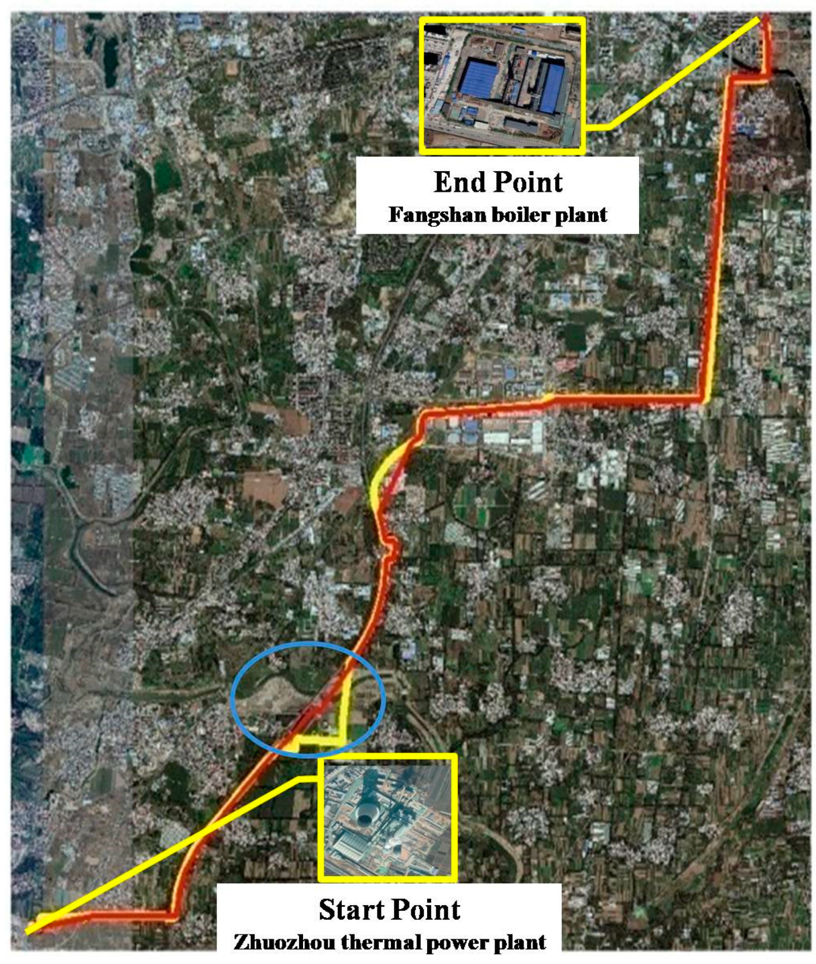
The ZF heating engineering project starts from the Zhuozhou thermal power plant in Hebei province and ends at the Fangshan boiler plant in Beijing. The locations of the start point and the end point are shown in Figure 1. From the image acquired from Google Earth, we can generally find that the landcover type of the study area are mainly high-grade highway (HGH), highway under construction (HUC), vegetation, water, and buildings.
2.2. The Principle of the Heating Route Selection
In this study, we focused on the route selection for the preliminary design phase, as the detailed route design for the construction phase required more sensitive data, such as the other pipe network distribution of the study area, which were difficult to acquire. So our primary task was to provide the general direction and critical nodes of an alternative optimum route for further refinement.
Heating route decision-making should follow several principles. We selected the regulations from the design code for the city heating network (CJJ 34-2010) [43]. The regulations related to our study are listed as follows:
- (1)
- Heating pipes through nonbuilt areas should be laid along the highway.
- (2)
- Heating pipes along the urban road should be parallel to the center line of the road and lay outside of the roadway. The same pipe should be laid only on one side of the street.
- (3)
- Heating pipes across the river, railway and road should perpendicularly intersect with each other. Under special circumstances, the intersection angle between the pipeline and railway or subway should not be less than 60°; the intersection angle between the pipeline and river or road should not be less than 45°.
There are regulations for the geological conditions: the selection of a heating pipe network is suitable to avoid unfavorable areas (i.e., soft soil areas, earthquake fault zones, landslide danger zones, and high underground water level areas). The minimum horizontal clearance and the minimum vertical clearance between the heating pipe and other pipes are also indicated in the design code.
In addition to regulations raised by the design code for the city heating network, the proprietor also treats cost as a significant consideration. The cost can be divided into two parts: one is related to the length of the route, and the other is related to the land use patterns. Obviously, the longer the route, the higher the cost. Regarding the land use patterns, if the construction occupies farm land or urban land or lands that have been used for other purposes, the occupancy fee and relocation fee should be considered in the total cost. Crossing water may be inevitable under some circumstances, it is a special case because shield technology may bring high cost. Generally, the cost per meter can be ranked as follows: cross water, cross building, cross vegetation, along HGH, along HUC. We treat the fitness function as the sum weight of all the pixels the route covers. The route with the minimum value of the fitness function should be the optimum route. Thus, the route selection can be transferred into a search for the minimum value of the fitness function as shown in Equation (1).
where p is the pixels the route covered. One can trace the corresponding row and column numbers of p in the binary images. IB is the building binary image where the building pixels are set to 1 while other pixels are set to 0. IV, IW, IHGH, and IHUC represent the binary images of vegetation, water, HGH, and HUC, respectively. wb, wv, ww, whgh, and whuc represent the weights of building, vegetation, water, HGH, and HUC, respectively. For example, if the location of p is a building pixel, then the IBp is 1, and IVp, IWp, IHGHp, and IHUCp are 0, so only the wb has an effect on the fitness function f.
ACO and CS are introduced to solve our route optimization problem. It is crucial to transfer the specific unresolved issues to the natural phenomena proposed by the algorithms. According to the regulations mentioned above, the heating route is preferred along the road. Therefore, it is a good idea to transfer the continuous image to discrete segments by breaking the roads into a number of segments at the intersections. The two endpoints of every segment are treated as the elementary entities (nodes). For example, in the ACO algorithm, the nodes can be compared to the cities; in the CS algorithm, the nodes can be compared to the location of eggs. Thus, we can derive a distance matrix from the node distribution as shown in Equation (2).
where i and j are the nodes in the study area. The distance matrix has characteristics as follows:
- (1)
- The distance of the same node equals 0, i.e., if i = j, di,j = 0;
- (2)
- The distance from node i to node j equals the distance from node j to node i, i.e., di,j = dj,i;
- (3)
- The distance between node i and node j can be calculated by the pixel number and the weight of the pixels. The formula can be expressed as Equation (3):
The equation illustrates the calculation method of the distance matrix. Suppose the start point is node i, and the end point is node j, where i and j belong to the same road, the distance between i and j is the sum weight of the pixels that the real curving segment covered. When the road is HGH, the distance can be calculated as (a) in Equation (3). When the road is the HUC, the distance can be calculated as (b) in Equation (3). Otherwise, if i and j belong to different roads, then the distance between i and j is the sum weight of pixels that the linear segment from i to j covered, as shown in (c) in Equation (3).
2.3. Data Organization and Management
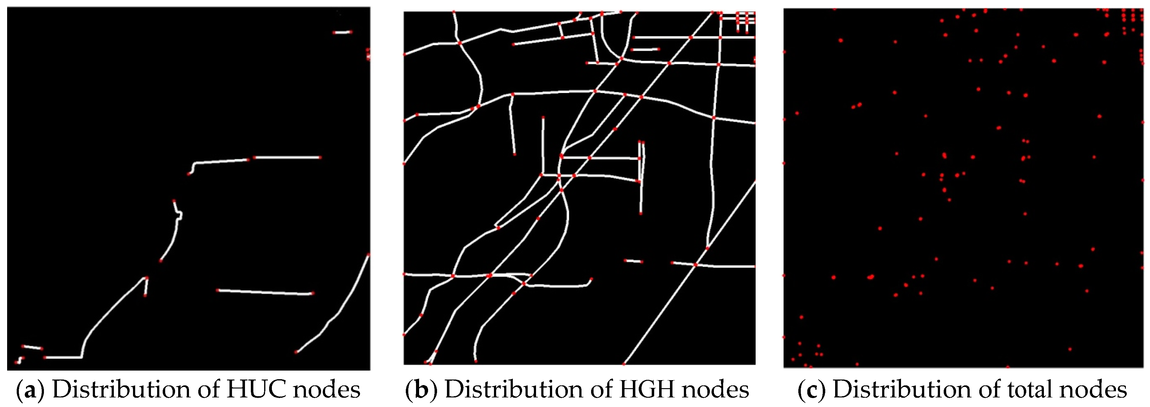
To execute intelligent route optimization, several data sets were collected and processed. The classification data were the essential data for our algorithms. We extracted 5 classification maps from the Google Earth image. Figure 2 shows the HGH, HUC, vegetation, water, and building binary images. Statistics show that there are 35 highways, 10 country roads, 128 building groups, 15 rivers or lakes, and the rest of the areas are regarded as vegetation.
According to the principle of heating route selection, the routes along the HUC or HGH have priority. Furthermore, because the cost of laying the heating line along the HUC is lower than along the HGH, the HUC has preference. Regarding vegetation, buildings and water, the occupancy fee and relocation fee may decrease successively. We assigned weights of different classifications by Delphi method. The weights of the land cover types were set to 0.0477, 0.0953, 0.190, 0.286, and 0.381 for HUC, HGH, vegetation, building groups, and water, respectively. In other words, we assigned 0.0477 to the HUC pixels in the HUC binary image, 0.0953 to the HGH pixels in the HGH binary image, 0.190 to the vegetation pixels in the vegetation binary image, 0.286 to the building pixels in the building binary image, and 0.381 to the water pixels in the water binary image. Therefore, the problem of this study was converted into searching for the minimum value of the sum weight of the pixels the route covered.
We extracted the two endpoints or intersections of the HUC and the HGH as nodes. From Figure 2, we found that there was no intersection in the HUC. However, there were several intersections among different HGH. Hence, we divided the HGH into segments by intersections. There were a total of 115 road segments (230 nodes). Based on the weights we assigned for the pixels, we calculated the distance between every two nodes. Thus, a 230 × 230 distance matrix was obtained. The distribution of the nodes in the study area is shown in Figure 3.
Referenced to [2,28], the optimum range of the variable (nodes) number should be no more than 75 for ACO and between 15 and 40 for CS. As it is unlikely that points far from the centre line will be chosen between the start point and the end point, we eliminated points outside of the 8 km buffer (Figure 4a). Meanwhile, the nodes at the intersections can be merged into one. As shown in Figure 4b, the 4 blue points at the intersection can be merged into one red point. Thus, the number of nodes was ultimately decreased to 35. It should be noted that the corresponding distance matrix and the covered pixels of the segments need to be updated simultaneously.
3. The Principle of the Intelligent Algorithms
3.1. Modified Ant Colony Optimization Algorithm
The ACO algorithm simulates the optimization of ant foraging behavior. It was originally used to solve the TSP. The TSP can be described as an oriented graph with N cities (nodes) (4):
where N = {1, 2, 3 … n}, A = {(i, j)|i, j ∈ N}. The distance between two cities can be expressed as (dij)n×n, while the fitness function can be expressed as Equation (5):
where w is an arrangement of the N cities. It is worth noting that the last city coincides with the first city, which means that the ant should return to the start point.
Regarding our specific heating route optimization problem, the efficient route was only confined to the segments from the start point to the end point. For example, as shown in Figure 5, there were 9 nodes in the graph, suppose the start point was 1, and the end point was 6. If the route one ant visited was 1 → 2 → 3 → 4 → 5 → 6 → 7 → 8 → 9 → 1, we only updated the pheromones from 1 to 6, i.e., τ12, τ23, τ34, τ45, τ56.
The value of the fitness function for one ant was the sum weight of the pixels from the start point to the end point. The cities visited after the end point were ignored. Also, taking Figure 5 as an example, the cost can be expressed as Equation (6):
where sij is the cost of the segment from i to j. If i and j belong to the same road, sij is the sum weight of the pixels covered by the real curving road. Otherwise, sij refers to the sum weight of pixels in the covered linear segment from i to j.
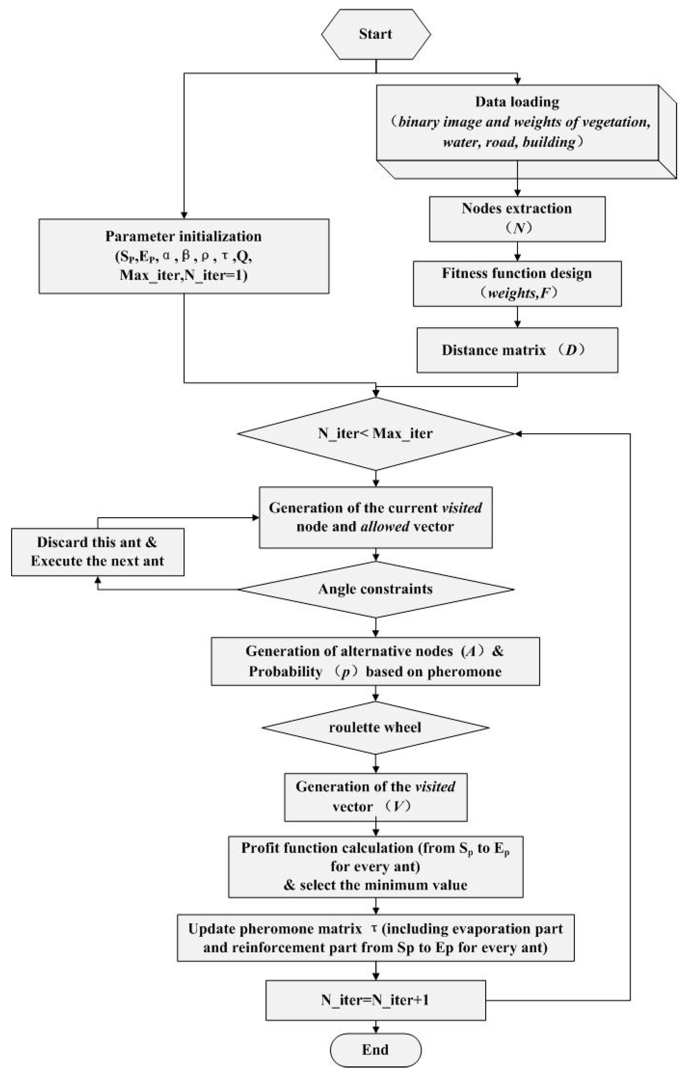
The modified procedure is shown as follows:
(1) Route Construction
Besides the predefined parameters of the original ACO algorithms, we also need to initialize the start point (SP), end point (EP), nodes (N), binary image of HUC (imgC), binary image of HGH (imgH), binary image of building (imgB), binary image of vegetation (imgV), binary image of water (imgW), and weights of every land cover type (w). Then, the distance matrix can be generated by Equation (3).
Every ant randomly selects a city and stores the visited cities in sequence into a vector named visited. The unvisited cities are also stored in a vector named allowed. The ant selects the next city to arrive at according to roulette wheels. The random probability is calculated following Equation (7).
where i and j are the start point and the end point of the segment.
is the intensity of the pheromone between i and j at time t. allowedk stores the yet unvisited cities. α and β are two constants, that can be described as the weighted values of pheromone and visibility, respectively. is the visibility of the segment, which can be expressed as the reciprocal of the distance between i and j as shown in Equation (8):
If j belongs to allowedk, is calculated by (a) in Equation (7), else, is set to 0 as (b) in Equation (7).
Different from the original ACO for TSP, the first element of the visited vector was the fixed start point for all ants, and the random generation of the visited vector was from the second point, and the valid points were from the first point (start point) to the end point (not necessarily visited all the 35 points).
In the original ACO, the nodes can be connected randomly, with the only constraint being that the nodes cannot be repeated in one route. However, in the heating route optimization problem, the route should also follow the constraints that the intersection angle between two adjacent segments should be no less than 90°, and there should not be crossovers among the segments. Therefore, when generating the visited vector, a stricter node-selection strategy should be conducted, and the pseudocode is listed as follows (Figure 6):
where Nallowed is the number of the residual nodes still unvisited. is one of the points from the allowed vector, while and are the current point and the previous point.
After this procedure, a subset of the allowed vector was derived in which all the candidate points conformed to the heating routing regulations. Therefore, the next point was chosen from the subset instead of the previous allowed vector. Inevitably, there was a condition that there were no available points for the next visited node before the ant reached the end point. If this happened, the ant was declared to be lost and was flagged to no longer participate in the updating and fitness function calculation.
(2) Pheromone Updating
The pheromone can be initialized as a constant for all the segments, as shown in Equation (9):
When all ants reach the end point, the path’s pheromone intensity should be updated, and the update is divided into two steps: one is the evaporation, and the other is the reinforcement. The formulation is shown in Equation (10):
where m is the number of ants (solutions), 0 < ρ <= 1 is the evaporation rate of the pheromones, is the pheromone released by the kth ant from path i to j. That is, the first part of the formula is the evaporation of the pheromone, while the second part is the reinforcement of the pheromone. It is worth noting that the pheromone updating was only focused on the segments between the start point and the end point.
(3) Iteration Stopping
There are two conditions for iteration stopping, one is the number of iterations reaching the value the user defined, and the other is all the ants following the same route (stagnant state).
The flowchart of the modified ACO is shown in Figure 7.
3.2. Modified Cuckoo Search Approach
The CS is inspired by the reproduction strategy of cuckoos. The algorithm uses three idealized rules:
- (1)
- Each cuckoo lays one egg at a time and dumps it in a random nest;
- (2)
- A fraction of the nests containing the best eggs, or solutions, will carry over to the next generation;
- (3)
- The number of nests is fixed and there is a probability that a host will discover an alien egg. If this occurs, the host can either discard the egg or build a new nest in a new location.
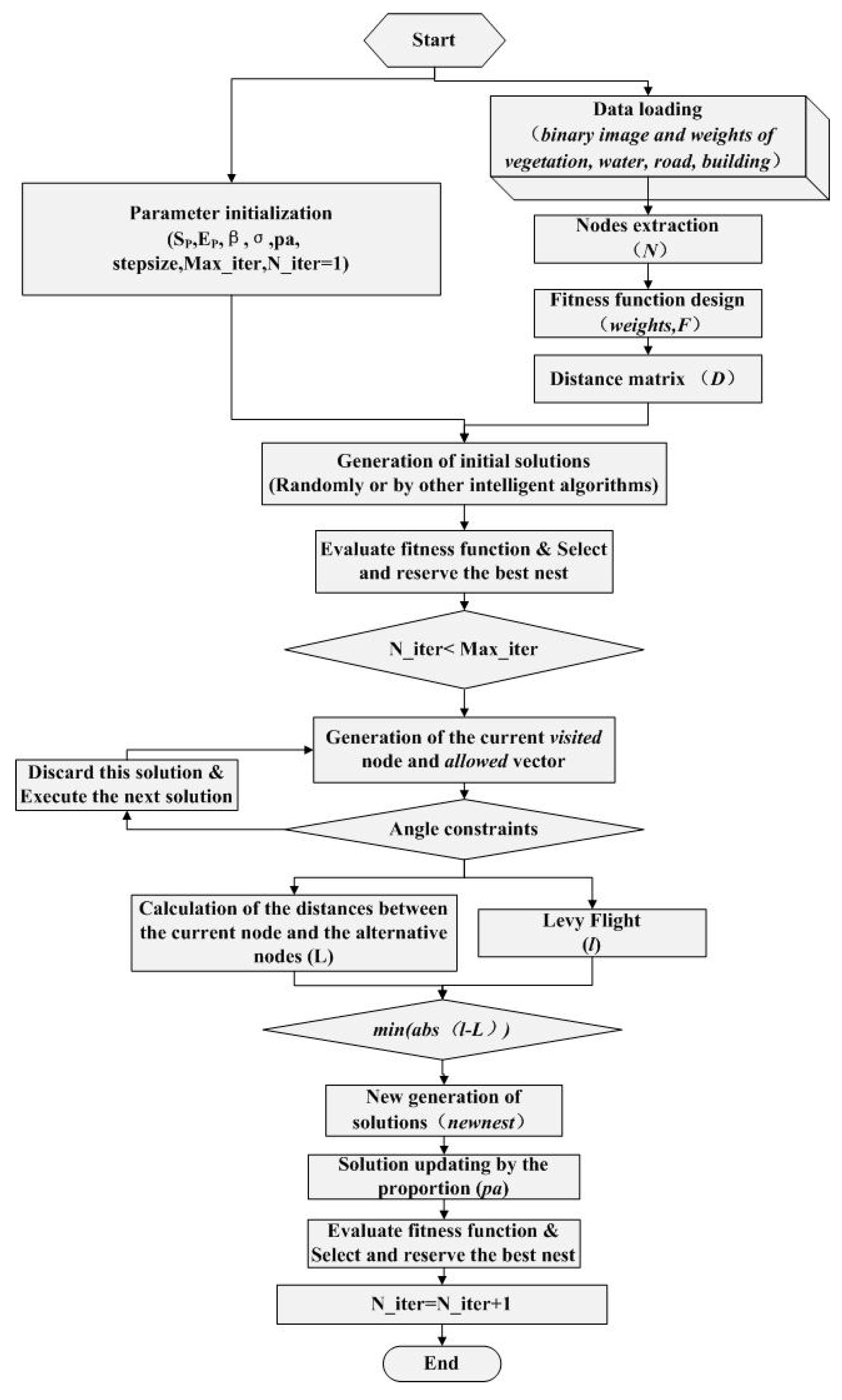
Because the original CS algorithm was designed to solving the continuous problems, there should be several modifications to suit the algorithm to the heating route selection problem. The modified procedure is shown as follows:
(1) Initialization
In this study, we set the dimension of the solution matrix as 5 × 35. The initial solutions can be given randomly or by other optimization algorithm, such as the modified ACO. The initial solutions should also follow the angle constraints like the modified ACO did.
Similar to the modified ACO, the start point (SP), end point (EP), nodes (N), binary image of HUC (imgC), binary image of HGH (imgH), binary image of building (imgB), binary image of vegetation (imgV), binary image of water (imgW), and the weights of every land cover type (w)were initialized. Then, the distance matrix can be generated by Equation (3).
Based on the initial solutions and the distance matrix, the best solution can be chosen and saved by comparing the value of the fitness function. Afterwards, the iterations were conducted and the new solutions by Lévy flights can be generated. The solution generation and updating were also confined from the start point to the end point.
(2) Updating the nests by Lévy flights
Lévy flight was executed when generating a new solution, and the updating formulation is expressed as Equation (11):
where and represent the nests or the egg locations at time t and time t + 1. represents the entry-wise operator. Because the search path hops randomly by Lévy flight, an adjustment called α was introduced according to the size of the problem, and α > 0. The formulation of the Lévy flight can be shown in Equation (12):
where β is often set as 1.5. The parameters ν and μ are the random numbers following a normal distribution, as shown in Equation (13):
where and can be calculated by Equation (14):
The Γ function can be expressed as Equation (15):
Regarding the specific heat routing problem, the nodes were discretely distributed. The distance by random Lévy flight maybe not exactly match the available nodes. Furthermore, the angle constraint should be considered as well. Referencing the modified ACO algorithm, we determined the alternative nodes by the pseudocode in Figure 6. Then, the distances between the current node and the alternative nodes were calculated, the one closest to the Lévy flight distance was selected, and the specific node was chosen as the next visited one. There was also a condition that no eligible point existed for the next generation. If this happened, the solution was declared invalid. After all the solutions were updated, the best solution of this generation was selected and saved by comparing the value of the fitness function.
(3) Updating the Nests if the Hosts Find the Eggs
A random matrix that with the same size as the nest matrix was generated and compared with the constant pa. Elements larger than pa should be updated by a random stepsize on condition that the angle constraint was satisfied.
(4) Iteration Stopping
There are two conditions for stopping iterations, one is the number of iterations reaching the value the user defined, and the other is all the solutions follow the same route (stagnant state).
The flowchart of the modified CS is shown in Figure 8.
3.3. Hybrid Ant Colony & Cuckoo Search (HACCS) Algorithm
From the studies mentioned above, we can conclude that the ACO algorithm is good at exploring promising areas of the TSP solution space. However, it is not skillful in fine-tuning as the CS algorithm. Meanwhile, the performance of the CS algorithm might be improved given good initial solutions. Therefore, in this study, we coupled the modified ACO algorithm with the modified CS algorithm, named HACCS algorithm. The HACCS combines the merits of ACO in exploring solution space and CS in refining solutions.
The HACCS algorithm includes two modules: the ACO module and the CS module. The ACO module was executed first to find the promising solution areas (global exploration) and transfer the 5 best solutions to the CS module as the initial solutions. Then, the CS module was used to find the better local optima (local exploitation). The flowchart is shown in Figure 9.
4. Results
In reality, the planning of the project was began in 2012, and the construction of the project was from 2017 to 2018. The decision making was a time consuming task required repeated negotiations with the planning department. Figure 10 shows the final route that was selected manually. The fitness function values of the manually selected route was 234.300.
To quantitatively evaluate the algorithms, we compared the results by the modified ACO, the modified CS, and HACCS with the same number of iteration. The results were compared with the route selected manually. Computer codes were developed in MATLAB for the algorithms.
4.1. Route Analysis by Modified ACO Algorithm
As there were a total of 35 nodes for the route search, we set 34 ants (solutions) for the route search, which meant that the size of the visited matrix was 34 × 35. The start point was set as the 1st node (column number: 41, row number: 1457), while the end point was set as the 29th node (column number: 1411, row number: 31). The pheromone index (α) was predefined as 1.0, the heuristic index (β) was 5.0, the evaporation index (ρ) was 0.5, and the initial pheromone value (τ) was 1.0 for all segments. To reinforce the pheromones, a 100 times (Q) magnification to the visibility of the segment (η) was added to the pheromone of the corresponding segment.
We set the number of iterations as 1000 for the modified ACO algorithm and repeated 20 times to verify its stability. The final fitness function values after 1000 iterations with 20 repetitions are shown in Figure 11. The average value was 240.620, while the best performer was 232.343. Compared to the fitness function values of the manually selected route (234.300), the modified ACO derived a decent solution. However, the stability was not good: among the 20 repetitions, there were 8 times the fitness function values were still high after 1000 iterations.
The detailed fitness function value distribution is shown in Figure 12. From the 3D diagram, we can find the convergence of the modified ACO algorithm was good. There was an 80% chance that the modified ACO algorithm can achieve the minimum value after no more than 400 iterations.
The best route is shown in Figure 13. The yellow line shows the manual route, the red line is the best route selected by the modified ACO. We found that the best route selected by the modified ACO preferred straight line instead of the right-angle as the manual route did. The reason may be the weights we predefined was not exactly conformed to reality. As to the our knowledge, the hypotenuse of a right triangle is less than the sum of its two sides. However, if the cost (weight multiplies length) of the two sides is less than the cost of the hypotenuse, then it is more inclined to choose the two sides of the right triangle, as the manual route did.
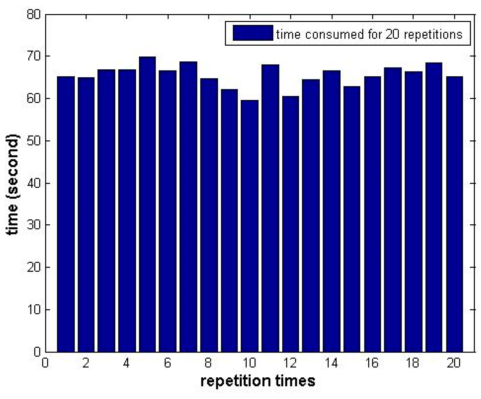
The elapsed time of 20 repetitions is shown in Figure 14. The average elapsed time was 65.46 s. Considering the 1000 iterations and 34 solutions for every run, the time consumed for one solution was approximately 1.93 ms.
4.2. Route Analysis by Modified CS Algorithm
Given the initial solutions, the modified CS can be executed individually. Here, we randomly generated 5 nests (solutions) for the route search as the initial solutions, so the size of the solution matrix was 5 × 35. The start point was set as the 1st node (column number: 41, row number: 1457), while the end point was set as the 29th node (column number: 1411, row number: 31). Only three parameters were predefined for CS: α (0.01), β (1.5) and pa (0.25).
We also set the number of iterations as 1000 for the modified CS algorithm and repeated 20 times to verify its stability. The final fitness function values after 1000 iterations with 20 repetitions are shown in Figure 15. The average value was 282.000 while the best performer was 244.247. Similar to the modified ACO, the stability of the modified CS was not quite well. Among the 20 repetitions, there were 15 times that the fitness function values were quite high after 1000 iterations.
Compared to the fitness function values of the modified ACO (232.343) and the manually selected route (234.300), the best performance (244.247) of the modified CS was not as good as the modified ACO. However, it was closer to the manually selected route. As shown in Figure 16, the yellow line shows the manual route, the red line is the best route of the modified CS. Both of them overlapped well except for the blue circle area. The reason could also be the weights we set was not exactly conformed to reality. If not considering the weights of the pixels, the straight lines are shortest between two points.
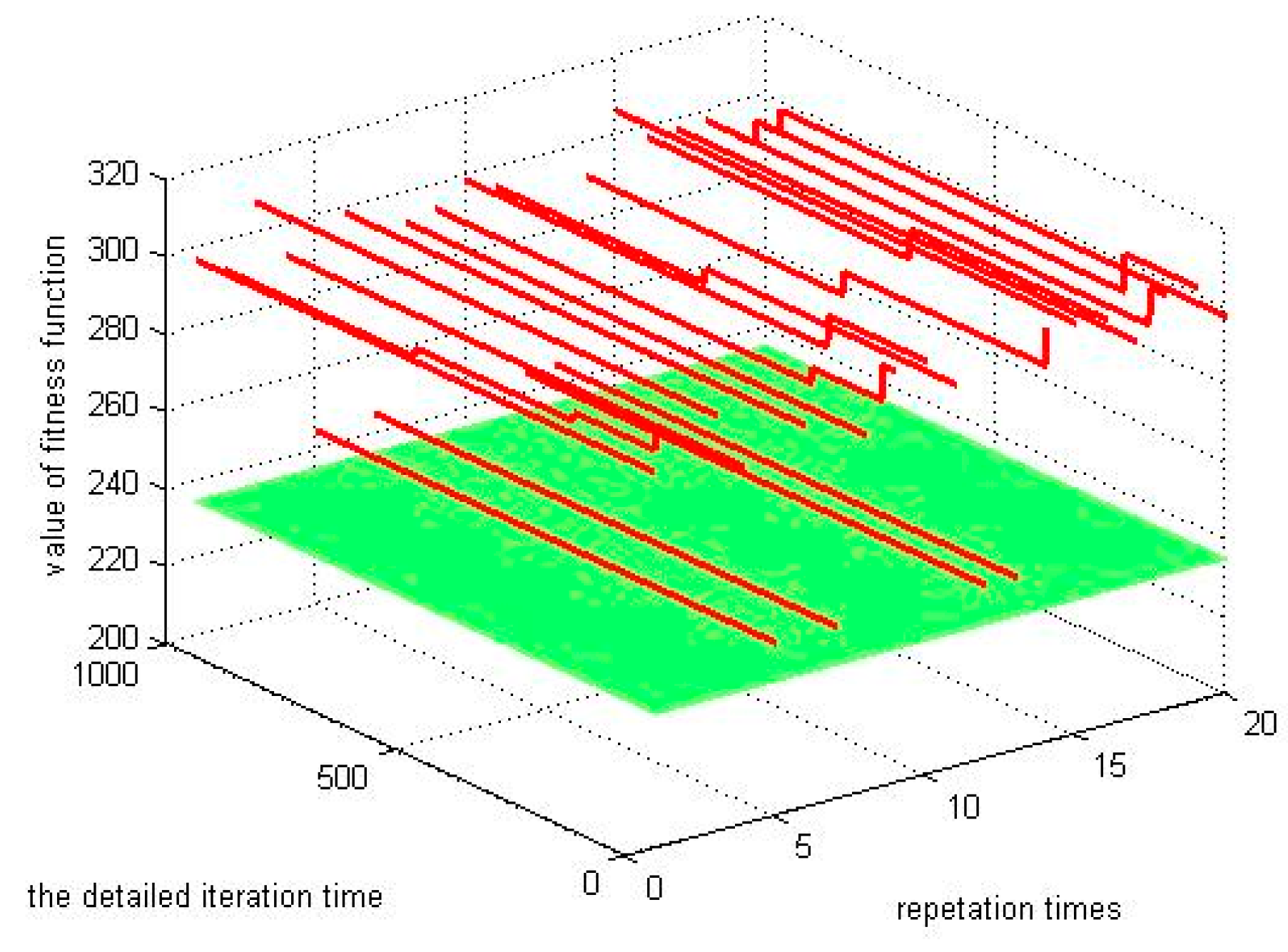
The detailed fitness function value distribution is shown in Figure 17. From the 3D diagram, we found that the convergence of the modified CS algorithm was not as good as the modified ACO. Although there was a 100% chance that the modified CS algorithm can achieve the minimum value after no more than 400 iterations, the final fitness value was still much higher than the manual selected route. This situation also confirmed the advantage of the CS in a local search, but not as well in a global search.
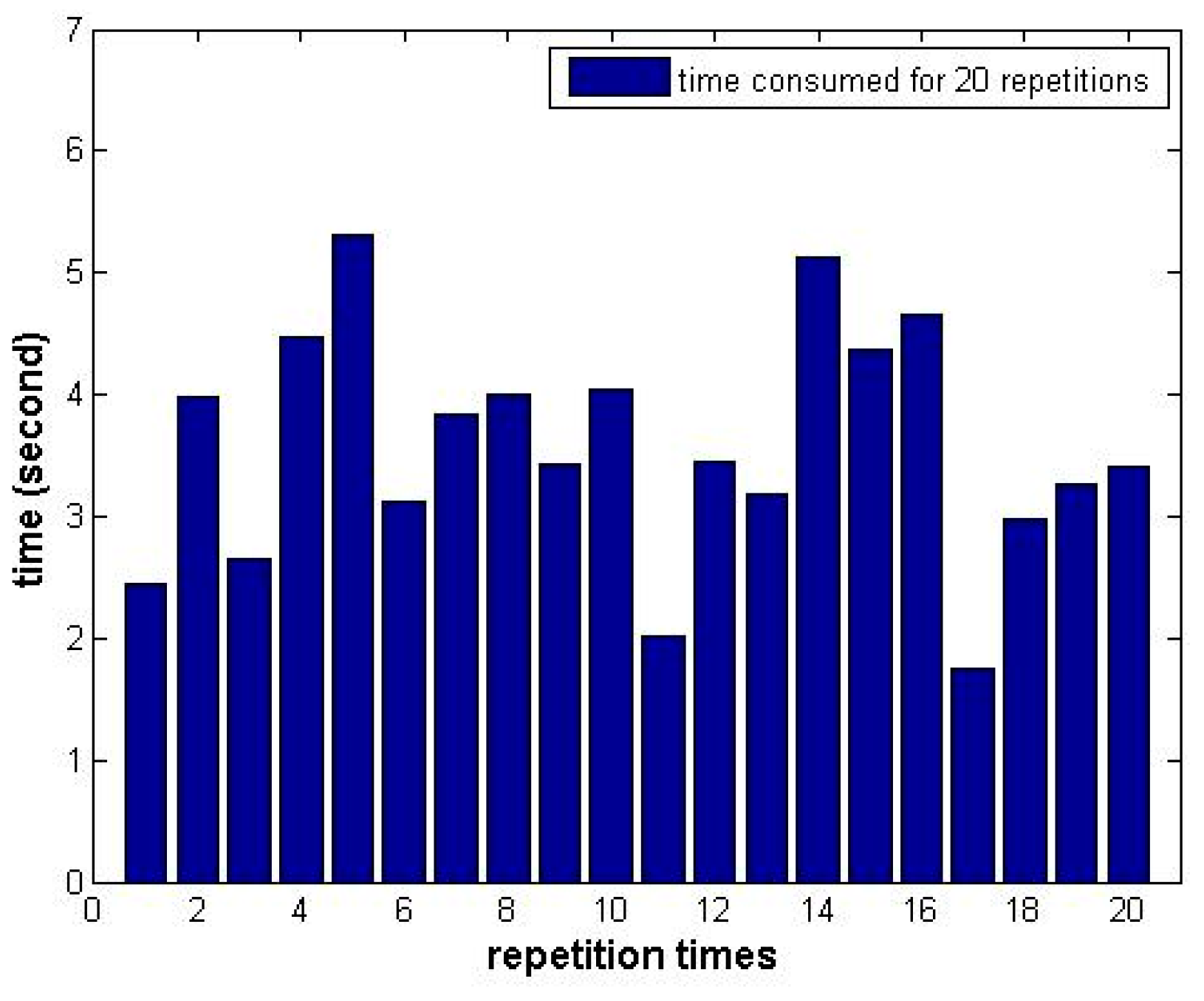
The elapsed time of 20 repetitions is shown in Figure 18. The average elapsed time was 3.97 s. Considering the 1000 iterations and 5 solutions for every run, the time consumed for one solution was approximately 0.794 ms, which was much more quickly than the modified ACO.
4.3. Route Analysis by HACCS Algorithm
Based on the work described in Section 4.1 and Section 4.2, we concluded that the modified ACO can escape from local optima relatively well but consumed more time. Meanwhile, the modified CS ran more quickly but easily stuck into the premature convergence. In this study, we proposed the hybrid algorithm(HACCS) that coupled the ACO and CS algorithms. HACCS was consisted of the modified ACO module and the modified CS module. To improve efficiency, we set the number of iterations as 400 and the repetition times as 20 for the ACO module and the CS module, according to the convergence study mentioned above.
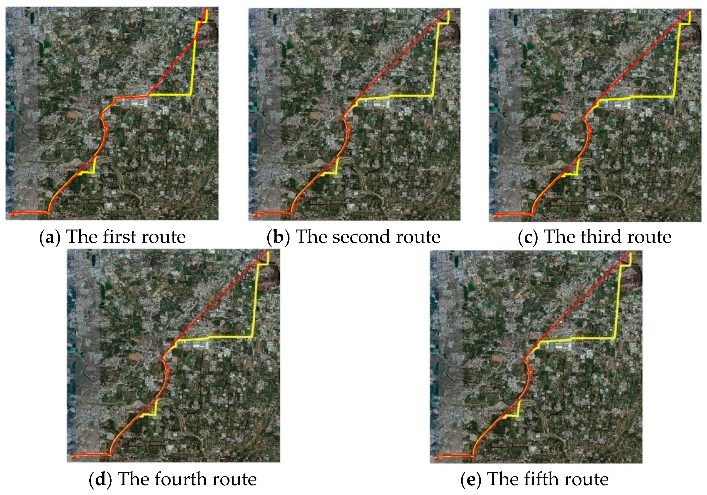
The 5 best routes by the ACO module are shown in Figure 19. The fitness function values were 232.343, 232.782, 232.782, 232.782, 232.877, respectively. Then, they were transferred to the CS module as the initial solutions. With the help of the optimized initial solutions, the performance of the modified CS would be improved.
Figure 20 shows the best route by the modified CS module. It is also the final best route by the HACCS. The red line was the best route by the HACCS, while the yellow line was the manual selected route. We found that the best route by HACCS was the same as the best route by the modified ACO.
The final fitness function values are shown in Figure 21. Because the initial solutions were optimized, the value of the algorithm was stable and maintained 232.343 for 20 repetitions.
Because the elapsed time for one solution was approximately 1.93 ms by the modified ACO, the time consumed for one solution was approximately 0.794 ms by the modified CS, considering the 400 iterations as well as the 34 solutions for ACO module and 5 solutions for CS module, the total time consumed for the HACCS was approximately 27.836 s, which was more quickly than the modified ACO (65.46 s).
5. Discussion
This study referenced state-of-the-art SI-based intelligent algorithms, specifically the ACO and CS algorithms. With the modifications of each algorithm and the hybrid strategy, we presented the modified ACO, the modified CS, as well as the HACCS algorithms to solve the heating route optimization problem. The proposed algorithms were applied to the ZF heating engineering project.
To verify the modified ACO and modified CS algorithms, we set the number of iterations as 1000 and the repetition times as 20. Comparing to the fitness function value of the manual route (234.300), the best route selected by modified ACO was 232.343, the average value was 240.620 for 20 repetitions, and the elapsed time for one solution was approximately 1.93 ms. There was an 80% chance that the modified ACO algorithm can achieve the minimum value after no more than 400 iterations. Meanwhile, the best route selected by modified CS was 244.247, the average value was 282.000 for 20 repetitions, and the elapsed time for one solution was approximately 0.794 ms. There was a 100% chance that the modified CS algorithm can achieve the minimum value after no more than 400 iterations. We concluded that the modified ACO can find the route with smaller fitness function value, while the modified CS can find the route overlapped to the manual selected route better. The modified CS ran more quickly but easily stuck into the premature convergence. According to the convergence study mentioned above, the HACCS was executed with a 400 iteration and 20 repetition for the ACO module and the CS module. The top five best routes by the ACO module was transferred to the CS module as the optimized initial solutions. The best route selected by the HACCS was the same as the modified ACO algorithm (232.343), but with higher efficiency and better stability.
In this study, we devoted to provide the general direction of an alternative optimum route for the preliminary design phase. With the help of our algorithms, we can give a quantitative assessment for the alternative routes. The features and innovations of this study lie in the following:
(1) The modification of the original ACO and CS algorithms to solve the heating route optimization problem.
By introducing high resolution remote sensing image and heating route selection principle, we extracted the critical discrete nodes, established the distance matrix and the fitness function. Additionally, the updating strategy was improved.
(2) The presentation of the HACCS algorithm.
By coupling of the ACO and CS algorithm, the advantage of the ACO in global search and the strength of the CS in fine-tuning can be fully displayed.
(3) The application of the HACCS for solving the route selection problem in reality
We proposed and applied the HACCS algorithm into the ZF heating route engineering project. The comparison and analysis showed that it is a feasible and effective way to solve practical route selection problems.
There are several improvements that we can focus on in the future. One is the improvement of the operational efficiency. By introducing parallel computing technology, the computing scale can be enlarged, and the computation time can be significantly shortened. The other is the 3D detailed route optimization with the support of the secondary data, such as other pipeline distribution maps, geological profiles, and the delicate DEM and DSM. Furthermore, with the help of 3D GIS technology, the interaction of the route and the users can be realized. Finally, we expect that the HACCS algorithm can be applied to route selection problems in broader engineering problems.
Author Contributions
Conceptualization, Y.Z., H.Z. and J.W.; Data curation, Y.Z. and M.H.; Methodology, Y.Z. and H.Z.; Software, Y.Z.; Supervision, Y.C., Q.L. and Z.S.; Writing—original draft, Y.Z.; Writing—review & editing, Y.Z., H.Z., Y.C., Q.L., Z.S. and J.W.
Funding
This research was funded by the National Key Research and Development Program, grant number 2018YFA0605503, and the Young Scientists Fund of the National Natural Science Foundation of China, grant number 41801257.
Acknowledgments
We gratefully acknowledge the anonymous reviewers for their insightful comments on the manuscript. The authors wish to thank Dorigo M et al. and Xin-She Yang et al. for providing the original program for ant colony optimization and cuckoo search. The authors wish to thank Tao Chen et al. from Beijing gas and heating engineering design institute for providing valuable suggestions on heating route planning regulations. The authors wish to thank Lei Zhang, and Kuisheng Yang from North China Power Engineering Co., Ltd. of China Power Engineering Consulting Group for the introduction of ZF heating engineering project.
Conflicts of Interest
The authors declare no conflicts of interest.
Abbreviations
| ACO | Ant Colony Optimization |
| ACS | Ant Colony System |
| ABC | Artificial Bee Colony |
| ASrank | Rank-based Ant System |
| CVRP | Capacitated Vehicle Routing Problem |
| CSA | Cuckoo Search Approach |
| DCS | Discrete Cuckoo Search |
| EAs | Evolutionary Algorithms |
| FA | Firefly Algorithm |
| GA | Genetic Algorithms |
| HACCS | Hybrid Ant Colony and Cuckoo Search |
| HGH | High-Grade Highway |
| HSA-CS | Hybrid Self-Adaptive CS |
| HUC | Highway Under Construction |
| IIWD | Improved Intelligent Water Drops |
| IWD | Intelligent Water Drops |
| LSHA | Local Search Hybrid Algorithm |
| MMAS | Max–Min Ant System |
| PSO | Particle Swarm Optimization |
| POHA | Post-Optimization Hybrid Algorithm |
| RKCS | Random-Key Cuckoo Search |
| SI | Swarm-Intelligence |
| TSP | Travelling Salesman Problem |
| ZF | Zhuozhou–Fangshan |
References
- Lawler, E.L.; Lenstra, J.K.; Kan, A.R.; Shmoys, D.B. The Traveling Salesman Problem: A Guided Tour of Combinatorial Optimization; Wiley: Chichester, UK, 1985. [Google Scholar]
- Shehab, M.; Khader, A.T.; Al-Betar, M. A survey on applications and variants of the cuckoo search algorithm. Appl. Soft Comput. 2017, 61, 1041–1059. [Google Scholar] [CrossRef]
- Eiben, A.E.; Smith, J.E. Introduction to Evolutionary Computing; Springer: Berlin/Heidelberg, Germany, 2003. [Google Scholar]
- Storn, R.; Price, K.V. Minimizing the real functions of the ICEC’96 contest by differential evolution. In Proceedings of the IEEE International Conference on Evolutionary Computation, Nagoya, Japan, 20–22 May 1996; pp. 842–844. [Google Scholar]
- Kirkpatrick, S.; Gelatt, C.D.; Vecchi, M.P. Optimization by simulated annealing. Science 1983, 220, 671–680. [Google Scholar] [CrossRef] [PubMed]
- Al-Betar, M.A. β-Hill climbing: An exploratory local search. Neural Comput. Appl. 2017, 28, 153–168. [Google Scholar] [CrossRef]
- Beni, G.; Wang, J. Swarm intelligence in cellular robotic systems. In Robots and Biological Systems: Towards a New Bionics, Proceedings of the NATO Advanced Workshop on Robots and Biological Systems, Toscana, Italy, 26–30 June 1989; Springer: Berlin/Heidelberg, Germany, 1993; pp. 26–30. [Google Scholar]
- Blum, C.; Merkle, D. Swarm Intelligence: Introduction and Applications, Natural Computing Series; Springer: Berlin/Heidelberg, Germany, 2008. [Google Scholar]
- Bolaji, A.L.; Al-Betar, M.A.; Awadallah, M.A.; Khader, A.T.; Abualigah, L.M. A comprehensive review: Krill herd algorithm (KH) and its applications. Appl. Soft Comput. 2016, 49, 437–446. [Google Scholar] [CrossRef]
- Dorigo, M.; Maniezzo, V.; Colorni, A. The Ant System: An Autocatalytic Optimizing Process. Available online: https://pdfs.semanticscholar.org/9649/211474dcfc3a9fd75e5208ffd21d9dcb9794.pdf (accessed on 15 March 2018).
- James, K.; Russell, E. Particle swarm optimization. In Proceedings of the 1995 IEEE International Conference on Neural Networks, Perth, WA, Australia, 27 November–1 December 1995; pp. 1942–1948. [Google Scholar]
- Karaboga, D. An Idea Based on Honey Bee Swarm for Numerical Optimization; Technical Report; Computer Engineering Department, Engineering Faculty, Erciyes University: Melikgazi, Turkey, 2005. [Google Scholar]
- Yang, X.-S. Nature-Inspired Meta Heuristic Algorithms; Luniver Press: Beckington, UK, 2008; pp. 242–246. [Google Scholar]
- Yang, X.-S.; Deb, S. Cuckoo search via Lévy flights. In Proceedings of the World Congress on Nature & Biologically Inspired Computing (NaBIC), Coimbatore, India, 9–11 December 2009; pp. 210–214. [Google Scholar]
- Shah-Hosseini, H. The intelligent water drops algorithm: A nature-inspired swarm-based optimization algorithm. Int. J. Bio-Inspired Comput. 2009, 1, 71–79. [Google Scholar] [CrossRef]
- Dorigo, M. Optimization, Learning and Natural Algorithms. Ph.D. Thesis, Dipartimento di Elettronica, Politecnico di Milano, Milano, Italy, 1992. (In Italian). [Google Scholar]
- Dorigo, M.; Maniezzo, V.; Colorni, A. Ant system: Optimization by a colony of cooperating agents. IEEE Trans. Syst. Man Cybern. Part B 1996, 26, 29–41. [Google Scholar] [CrossRef] [PubMed]
- Bullnheimer, B.; Hartl, R.F.; Strauss, C. A new rank-based version of the ant system: A computational study. Cent. Eur. J. Oper. Res. Econ. 1999, 7, 25–38. [Google Scholar]
- Stützle, T.; Hoos, H. MAX–MIN ant system and local search for the traveling salesman problem. In Proceedings of the 1997 IEEE International Conference on Evolutionary Computation (ICEC’97), Indianapolis, IN, USA, 13–16 April 1997; pp. 309–314. [Google Scholar]
- Stützle, T.; Hoos, H. Max–min ant system. Future Gener. Comput. Syst. 2000, 16, 889–914. [Google Scholar] [CrossRef]
- Dorigo, M.; Gambardella, L.M. Ant colony system: A cooperative learning approach to the traveling salesman problem. IEEE Trans. Evol. Comput. 1997, 1, 53–66. [Google Scholar] [CrossRef]
- Yu, B.; Yang, Z.-Z.; Yao, B. An improved ant colony optimization for vehicle routing problem. Eur. J. Oper. Res. 2009, 196, 171–176. [Google Scholar] [CrossRef]
- Tuba, M.; Jovanovic, R. Improved ACO algorithm with pheromone correction strategy for the traveling salesman problem. Int. J. Comput. Commun. 2013, 8, 477–485. [Google Scholar] [CrossRef]
- Chen, S.-M.; Chien, C.-Y. Solving the traveling salesman problem based on the genetic simulated annealing ant colony system with particle swarm optimization techniques. Expert Syst. Appl. 2011, 38, 14439–14450. [Google Scholar] [CrossRef]
- Deng, W.; Chen, R.; He, B.; Liu, Y.Q.; Yin, L.F.; Guo, J.H. A novel two-stage hybrid swarm intelligence optimization algorithm and application. Soft Comput. 2012, 16, 1707–1722. [Google Scholar] [CrossRef]
- Mahi, M.; Baykan, Ö.K.; Kodaz, H. A new hybrid method based on particle swarm optimization, ant colony optimization and 3-opt algorithms for traveling salesman problem. Appl. Soft Comput. 2015, 30, 484–490. [Google Scholar] [CrossRef]
- Zhang, X.; Tang, L. A new hybrid ant colony optimization algorithm for the traveling salesman problem. In Proceedings of the 4th International Conference on Intelligent Computing, Shanghai, China, 15–18 September 2008; pp. 148–155. [Google Scholar]
- Kaabachi, I.; Jriji, D.; Krichen, S. A DSS Based on Hybrid Ant Colony Optimization Algorithm for the TSP. In Proceedings of the International Conference on Artificial Intelligence and Soft Computing, Zakopane, Poland, 11–15 June 2017; pp. 645–654. [Google Scholar]
- Liu, W.; Zhou, Y. An effective hybrid ant colony algorithm for solving the traveling salesman problem. In Proceedings of the 2010 International Conference on Intelligent Computation Technology and Automation, Changsha, China, 11–12 May 2010. [Google Scholar]
- Yang, X.-S.; Deb, S. Engineering optimisation by cuckoo search. Int. J. Math. Model. Numer. Optim. 2010, 1, 330–343. [Google Scholar] [CrossRef]
- Gandomi, A.H.; Yang, X.-S.; Alavi, A.H. Cuckoo search algorithm: A metaheuristic approach to solve structural optimization problems. Eng. Comput. 2013, 29, 17–35. [Google Scholar] [CrossRef]
- Chiroma, H.; Herawanb, T.; Fister, I., Jr.; Fister, I.; Abdulkareem, S.; Shuib, L.; Hamza, M.F.; Saadi, Y.; Abubakar, A. Bio-inspired computation: Recent development on the modifications of the cuckoo search algorithm. Appl. Soft Comput. 2017, 61, 149–173. [Google Scholar] [CrossRef] [Green Version]
- Mlakar, U.; Fister, I., Jr.; Fister, I. Hybrid self-adaptive cuckoo search for global optimization. Swarm Evol. Comput. 2016, 29, 47–72. [Google Scholar] [CrossRef]
- Saelim, A.; Rasmequan, S.; Kulkasem, P.; Chinnasarn, K.; Rodtook, A. Migration planning using modified cuckoo search algorithm. In Proceedings of the 13th International Symposium on Communications and Information Technologies (ISCIT), Surat Thani, Thailand, 4–6 September 2013; pp. 621–626. [Google Scholar]
- Ouaarab, A.; Ahiod, B.; Yang, X.-S. Discrete cuckoo search algorithm for the travelling salesman problem. Neural Comput. Appl. 2014, 24, 1659–1669. [Google Scholar] [CrossRef]
- Ouaarab, A.; Ahiod, B.; Yang, X.-S. Random-key cuckoo search for the travelling salesman problem. Soft Comput. 2015, 19, 1099–1106. [Google Scholar] [CrossRef]
- Abu-Srhan, A.; Daoud, E.A. A hybrid algorithm using a genetic algorithm and cuckoo search algorithm to solve the traveling salesman problem and its application to multiple sequence alignment. Int. J. Adv. Sci. Technol. 2013, 61, 29–38. [Google Scholar] [CrossRef]
- Teymourian, E.; Kayvanfar, V.; Komaki, G.H.M.; Zandieh, M. Enhanced intelligent water drops and cuckoo search algorithms for solving the capacitated vehicle routing problem. Inf. Sci. 2016, 334–335, 354–378. [Google Scholar] [CrossRef]
- Feng, Y.; Wang, G.; Feng, Q.; Zhao, X. An effective hybrid cuckoo search algorithm with improved shuffled frog leaping algorithm for 0–1 knapsack problems. Comput. Intell. Neurosci. 2014, 2014, 1–17. [Google Scholar] [CrossRef] [PubMed]
- Feng, Y.; Wang, G.; Gao, X. A novel hybrid cuckoo search algorithm with global harmony search for 0–1 knapsack problems. Int. J. Comput. Intell. Syst. 2016, 9, 1174–1190. [Google Scholar] [CrossRef]
- Alkhateeb, F.; Abed-alguni, B.H. A hybrid cuckoo search and simulated annealing algorithm. J. Intell. Syst. 2017. [Google Scholar] [CrossRef]
- Elkhechafi, M.; Hachimi, H.; Elkettani, Y. A new hybrid cuckoo search and firefly optimization. Monte Carlo Methods Appl. 2018, 24, 71–77. [Google Scholar] [CrossRef]
- People’s Republic of China Ministry of Housing and Urban-Rural Development. Design Code for City Heating Network (CJJ 34-2010); China Building Industry Press: Beijing, China, 2011.
Figure 1.
The location of the start point and end point of the ZF heating engineering project.

Figure 2.
Classification maps of the study area.

Figure 3.
The distribution of the nodes in the study area.

Figure 4.
Reduction of nodes by buffering and merging.

Figure 5.
A sketch map with nine nodes.

Figure 6.
Pseudocode for intersection angle constraints.

Figure 7.
Flowchart of the modified ACO.

Figure 8.
Flowchart of the modified CS.

Figure 9.
Flowchart of HACCS.

Figure 10.
The manually selected heating route.

Figure 11.
The final fitness function values after 1000 iterations with 20 repetitions of the modified ACO.
Figure 11.
The final fitness function values after 1000 iterations with 20 repetitions of the modified ACO.

Figure 12.
The detailed fitness function values of 1000 iterations with 20 repetitions of the modified ACO.
Figure 12.
The detailed fitness function values of 1000 iterations with 20 repetitions of the modified ACO.

Figure 13.
The best route of the modified ACO.

Figure 14.
The time consumed for different iteration times of the modified ACO.

Figure 15.
The final fitness function values after 1000 iterations with 20 repetitions of the modified CS.
Figure 15.
The final fitness function values after 1000 iterations with 20 repetitions of the modified CS.

Figure 16.
The best route of the modified CS.

Figure 17.
The detailed fitness function values of 1000 iterations with 20 repetitions of the modified CS.
Figure 17.
The detailed fitness function values of 1000 iterations with 20 repetitions of the modified CS.

Figure 18.
The time consumed for different iteration times of the modified CS.

Figure 19.
Top 5 routes of the modified ACO module.

Figure 20.
The best route of the HACCS.

Figure 21.
The final fitness function values with 20 repetitions of the HACCS.

© 2018 by the authors. Licensee MDPI, Basel, Switzerland. This article is an open access article distributed under the terms and conditions of the Creative Commons Attribution (CC BY) license (http://creativecommons.org/licenses/by/4.0/).
Share and Cite
MDPI and ACS Style
Zhang, Y.; Zhao, H.; Cao, Y.; Liu, Q.; Shen, Z.; Wang, J.; Hu, M. A Hybrid Ant Colony and Cuckoo Search Algorithm for Route Optimization of Heating Engineering. Energies 2018, 11, 2675. https://doi.org/10.3390/en11102675
AMA Style
Zhang Y, Zhao H, Cao Y, Liu Q, Shen Z, Wang J, Hu M. A Hybrid Ant Colony and Cuckoo Search Algorithm for Route Optimization of Heating Engineering. Energies. 2018; 11(10):2675. https://doi.org/10.3390/en11102675
Chicago/Turabian StyleZhang, Yang, Huihui Zhao, Yuming Cao, Qinhuo Liu, Zhanfeng Shen, Jian Wang, and Minggang Hu. 2018. "A Hybrid Ant Colony and Cuckoo Search Algorithm for Route Optimization of Heating Engineering" Energies 11, no. 10: 2675. https://doi.org/10.3390/en11102675
Note that from the first issue of 2016, this journal uses article numbers instead of page numbers. See further details here.