Neural Extended State Observer Based Intelligent Integrated Guidance and Control for Hypersonic Flight


Aerospace Engineering Department, College of Aerospace Science and Engineering, National University of Defense Technology, Changsha 410073, China
*
Authors to whom correspondence should be addressed.
Energies 2018, 11(10), 2605; https://doi.org/10.3390/en11102605
Submission received: 24 August 2018
/
Revised: 26 September 2018
/
Accepted: 26 September 2018
/
Published: 29 September 2018
Abstract
:Near-pace hypersonic flight has great potential in civil and military use due to its high speed and low cost. To optimize the design and improve the robustness, this paper focuses on the integrated guidance and control (IGC) design with nonlinear actuator dynamics in the terminal phase of hypersonic flight. Firstly, a nonlinear integrated guidance and control model is developed with saturated control surface deflection, and third-order actuator dynamics is considered. Secondly, a neural network is introduced using an extended state observer (ESO) design to estimate the complex model uncertainty, nonlinearity and disturbance. Thirdly, a command-filtered back-stepping controller is designed with flexible designed sliding surfaces to improve the terminal performance. In this process, hybrid command filters are implemented to avoid the influences of disturbances and repetitive derivation, meanwhile solving the problem of unknown control direction caused by nonlinear saturation. The stability of the closed-loop system is proved by the Lyapunov theory, and the controller parameters can be set according to the relevant remarks. Finally, a series of numerical simulations are presented to show the feasibility and validity of the proposed IGC scheme.
1. Introduction
Since the 1980s, integrated guidance and control (IGC) has been the subject of lots of studies for tactical missiles, space shuttles and hypersonic flight vehicles. Firstly, the conventional design is not able to produce an optimal overall system. Because the guidance and control system is formed in two independent loops with different operation frequencies, the original performance objectives are lost when the two control loops are iteratively incorporated. Secondly, in order to improve the closed-loop performance, the modern guidance and control (G&C) design has involved various techniques such as sliding mode control, adaptive control, disturbance rejection control, anti-windup control, etc., because the system dynamics is obviously characterized by strong states coupling, imprecisely known aerodynamics, complex internal uncertainties and external disturbances, especially in hypersonic flight. Consequently, the IGC design has provided better solutions in terms of low cost, modular growth, design flexibility, simple logistics and has attracted great interest from researchers.
Schierman et al. [1] introduced an integrated adaptive guidance and control (IAG&C) program for Boeing’s X-40A. The development of future autonomous launch platforms will benefit from integrating trajectory reshaping with the essential elements of control reconfiguration and guidance adaptation. Shima et al. [2] considered the actuator dynamics as an important part of the integrated missile guidance and control system in a low-order element. Furthermore, two first-order actuators are considered in the IGC model of dual-control missiles in [3,4]; however, the controller complexity becomes staggering. Nevertheless, the true missile dynamics has high order for second- or third-order actuator dynamics. In [5], the sliding surface of a sliding mode integrated missile guidance and control is formed by Predicted-Impact-Point (PIP) heading error, and then a terminal second-order sliding mode control is designed to achieve the convergence in a finite time without chattering. In [6,7,8,9], an impact angle constraint sliding surface is proposed to extend the application and improve the terminal performance of IGC design. Disturbance observer has been widely used in dynamic model compensation, and the design of ESO has good flexibility with respect to its general form. The nonlinear ESO-based controller in [10] has better performance under complex uncertainties and measurement noises than linear ESO in [11] for missile guidance and control systems, while the nonlinear ESO has more parameters to tune. Huang et al. [12] used a nonlinear disturbance observer to estimate the nonlinearities, uncertainties, disturbances and compensate the dynamic model; thus, the undesired chattering in control signals is depressed and the robustness of closed-loop system is enhanced. Guo et al. [13] employed the ESOs to estimate indirectly measured states and cancel out various parametric uncertainties.
Neural networks are capable of providing arbitrarily good approximations of prescribed functions of a finite number of real variables in [14]. Application to dynamic system modeling, nonlinear complex valued signal processing associated with the radial basis function (RBF) neural network are described by Wu et al. [15]. In [16], direct neural control is proposed to deal with the input nonlinearity in the model of a hypersonic vehicle. An adaptive neural network is employed to estimate the structure uncertainties, and then a back-stepping controller is proposed to guarantee the uniform asymptotic stability of the uncertain system in [17]. In [18], RBF neural network approximation is combined with an adaptive back-stepping technique to achieve boundedness of all closed-loop system states. In [19], RBF neural networks are applied to approximate the lumped unknown nonlinearities to satisfy robustness against system uncertainties for a constrained flexible air-breathing hypersonic vehicle. Nonlinear saturation is modelled as a non-smooth function, and approximated with a smooth function with bounded error in backstepping controller design in [20]. Nussbaum function is used when differentiating the approximate function to guarantee the closed-loop stability. Chen et al. [21,22] introduced Nussbaum functions to compensate the nonlinear term due to differentiating the saturated control input and solve the problem of unknown control direction. In [22], a novel Nussbaum function gain-based controller is proposed for systems with multiple unknown actuator directions and time-varying nonlinearities.
To simplify the implementation and satisfy the constraint in back-stepping control techniques, a command filter is introduced. Farrell et al. [23] first introduced the command-filtered back-stepping technique to get the time derivatives of the virtual control signals, and it is feasible for high-order dynamic system. In [24,25], a low-pass command filter is employed to construct the derivative of virtual control input in dynamic surface control. It solves the problem of “explosion of complexity” caused by the repeated differentiations of the virtual control signals in the missile IGC design. The performance of command filter-based back-stepping control scheme significantly improves in stability and steady-state tracking accuracy, while the analysis via singular perturbation theory is made in detail in [26]. Xu et al. [27] proposed a second-order nonlinear command filter to directly impose magnitude and rate limitation on the control input. Wang et al. [28] proposed composite command-filtered back-stepping control for an ESO compensating IGC model with second-order actuator, and a Nussbaum function gain-based command filter was developed to deal with the control input constraints.
In brief, this work is motivated by (1) integrated guidance and control design, (2) complex uncertainty and disturbance estimate using an improved extended state observer based on neural network, (3) composite command-filtered back-stepping control with nonlinear constraint. This paper proposes a novel IGC approach to synthetically enhance the stability and robustness of an overall closed-loop system. Then, the application for hypersonic flight is able to be studied and discussed more practically and effectively.
The paper is organized as follows: in Section 1, the representative study in integrated guidance and control design are summarized, the control technique involved is introduced. In Section 2, an integrated guidance and control model in the terminal phase of hypersonic flight is developed with high-order actuator dynamics, and the control surface deflection is constrained by magnitude saturation. In Section 3, a neural extended state observer (NESO) is designed to synthetically estimate the complex uncertainty and time-varying disturbance, and three NESOs are used in different channels. In Section 4, a hybrid command-filtered back-stepping controller is designed. Command filters based on tracking differentiators are used to get the derivate of virtual inputs to avoid chattering, and a command filter based on the Nussbaum function is introduced when differentiating the saturated control input with unknown control direction. In Section 5, the stability of closed-loop system is analyzed by the Lyapunov theory, and the controller parameters can be set by relevant principles in the proof. In Section 6, numerical simulations in five scenarios, and Monte Carlo simulations of initial flight states, measurement noises, aerodynamics coefficients are presented to verify the proposed design in widely practical situation. Finally, in Section 7, all the above work is concluded.
2. IGC Model
In this section, the integrated guidance and control model in the terminal phase is developed with actuator dynamics. Figure 1 shows the planar geometry under inertial coordinate system without earth rotation. is the flight velocity, is the distance between the mass center and the landing point, is the angle between line of sight (LOS) and local horizon, is the flight path angle, is the angle of attack (AOA) and is the control surface deflection. The angle directions of and shown in Figure 1 are negative and is positive.
The state vector is chosen as , and the control surface deflection is saturated as . Then the state space form of integrated guidance and control model can be built as follows:
where are time-varying disturbances in different channels. The nonlinear functions and are depicted as follows:
In hypersonic flight, control-oriented forms of force and moment functions are introduced with curve-fitted approximations in Appendix A. The lift force can be simplified into two parts: , and in Equations (2a) and (2b) are the unified form of the parts, where is the mass. The aerodynamics moment is also described as two parts: , both are unified by the moment of inertia with respect to body z-axis : in Equation (2c). The high-order nonlinearity and states coupling mainly caused by aerodynamics coefficients uncertainties are synthesized as .
The nonlinear saturation characteristic of the actuator in Equation (1c) can be modeled as:
where is the maximum value of control surface deflection. The saturated can be approximated by a smooth function defined as:
then , is the small approximation error.
The actuator dynamics is considered to be a first order inertial element and a second-order element. It is expressed with the following transfer function:
where is time constant, is damping rate, is natural frequency and is constant gain.
3. Neural Extended State Observer
The extended state observer is widely implemented, with a simple structure and good estimation accuracy. Considering the following system with uncertainty and time-varying disturbance:
The basic idea of ESO is to estimate the synthetical disturbances . As the introduction section states, neural networks have good approximation performance in dealing with complex system uncertainties and disturbances. To compensate the complex aerodynamics uncertainties and time-varying disturbances in the IGC model, the technique of the extended state observer is exploited with a neural network.
Defining , as the states of NESO to estimate, respectively, and , and the estimate error of as , then the state space model of NESO is designed as follows:
where is the idea weight, is a vector of Gaussian functions, is the construction error of neural network observer.
is the center of the Gaussian functions vector, d is the affect size. By employing the -modification type of adaptation law, the weight vector can be functioned as:
where is constant, is gain. Defining as the reference signal of , then the tracking error can be expressed as .
In the integrated guidance and control design, three NESOs are used to compensate the synthetical disturbances in Equation (1), the estimate results are, respectively, .
4. Hybrid Command-Filtered Controller
In this section, a hybrid command-filtered back-stepping sliding mode controller is designed to achieve LOS rate convergence based on the estimate results of NESOs. Three low-pass filters are used to get one-order derivatives of virtual control input; the Nussbaum function is introduced to deal with the nonlinear saturation of control surface deflection with one-order auxiliary dynamics, and then a nonlinear third-order differentiator is implemented in the terminal sliding mode control.
Step 1: The first sliding surface is defined as . The virtual control input is designed according to proportional reaching law with positive constant .
Step 2: The second sliding surface is chosen as , and the virtual control input is obtained by the following control law, like in Step 1:
where is the derivative of . Directly differentiating with respect to time results in chatter and peak of the virtual control signal, so a low-pass command filter is introduced to get the derivative:
where is the positive time constant. The state error produced by Equation (12) is defined as , which can be sufficiently small when is appropriately set, thus replacing with . A low-pass filter in the same form as Equation (12) is used to avoid directly differentiating .
Then the error produced by the low-pass Equation (13) can be expressed as .
Step 3: In this step, there are two sub-steps to deal with the nonlinear saturation of control surface deflection.
Firstly, the virtual control input is designed to achieve the convergence of under the following control law:
Secondly, existing a sliding surface , its derivative with respect to time is depicted as:
where is obtained by the following low-pass filter with an error under time constant :
To get the first-order derivative , is passed through a low-pass filter with time constant .
In the process of reaching the law design of , the control direction is unknown because of saturation. A Nussbaum function command filter is introduced to design the virtual control input. The Nussbaum function is defining with the following properties:
Then the virtual control input is established as follows:
According to the above properties in Equation (18), the following Nussbaum function is implemented:
The parameter is set as an adaptive parameter according to the following principle:
In the end, a third-order differentiator is used as a command filter to get first- and second-order derivatives of the virtual control input :
where , the error between and can be sufficiently small through choosing suitable .
Step 4: The task of tracking is completed by a terminal sliding mode controller. From the second order dynamics in Equation (5), the following model is derived:
The model uncertainty and the time-varying disturbance are bounded by positive constants :
By defining error vector with , and its derivative can be written as . Then the following nonlinear sliding mode surface is designed:
In Equation (26), is a constant vector, and is determined by the following nonlinear function:
where is the convergence time of the terminal sliding mode controller.
Finally, the control input is designed as follows:
5. Stability Analysis
The tracking error of each step is depicted as , and differentiating them with respect to time:
The following Lyapunov function is chosen:
Differentiating the actuator dynamics related part of Equation (24) with respect to time:
The differentiator can be set appropriately such that , is a small positive constant, and is bounded. There exists a positive constant K that yields to:
Through differentiating Equation (30) and combining Equation (32), we have:
If defining the following bounds:
where , , , , .
According to the Young’s inequality, Equation (36) can be rewritten as follows:
Remark 1.
There exists a constant, then the following inequality is yielded to:
Integrating Equation (36) directly, then we have:
According to the proof in [22],is bounded, andis bounded, which implies that all the error is bounded.
6. Numerical Simulations
In this section, numerical simulations under five scenarios are provided to illustrate the control schemes proposed in the previous sections. First of all, the initial flight condition in terminal phase is set as follows:
The IGC model is built in the following first three scenarios with aerodynamics coefficients based on table in Appendix A. The aerodynamics coefficients in Scenario 4 (S4) and Scenario 5 (S5) are the same as Scenario 3 (S3). The control surface deflection is saturated within , and the third-order actuator dynamics is given by the following transfer function:
Scenario 1:
Scenario 2:
Scenario 3:
Scenario 4:
Furthermore, the un-modeled measurement uncertainty of is considered to be a first order transfer function with gain , and time constant .
Scenario 5:
Dead-zone is also part of control input nonlinearity, which can be defined by the following piecewise function of :
The time-varying disturbances in different channels of IGC model are given as follows:
Secondly, the three NESOs in Equation (7) are set. According to the form of nonlinear function to be estimated, the first neural network input is chosen as . The elements of the center vector are set based on the bound of the states.
The second neural network input is chosen as , according to the bound of the states, the following center vector is employed:
The third neural network input is chosen as , according to the bound of the states, the following center vector is employed:
The gains on estimate error in Equation (7) are set with .
Thirdly, the proportional reaching law of each step in Section 4 is set with constants . The low-pass command filters are built with time constants . The third-order differentiator in Equation (23) is set with . The Nussbaum function-based command filter is confirmed by Equation (22) with . The terminal sliding surface in Equation (26) is determined by , and the uncertainty and time-varying disturbance in Equation (28) are bounded by .
6.1. Nominal Simulation
The nominal simulation results of Scenario 1 (S1) indicate the feasibility of the proposed method. As Figure 2a shows, LOS rate finally converges to zero under the saturated control surface deflection. In Figure 2d, the control surface deflection of the IGC scheme is well bounded within . The state estimate errors of NESO converge well in very small range, the NESO can estimate the system states with good accuracy, and all the states converge under saturated control surface deflection. The results indicate that the proposed control scheme performs very well.
6.2. Comparison Simulations
Scenario 2 (S2) and Scenario 3 (S3) are compared to test the performance of NESO-based IGC under large aerodynamics coefficient uncertainties. In S2, contains nonlinear items of AOA, while are also nonlinear functions of AOA and pitch angle rate. In S3, are influenced by control surface deflection. Besides, simulation in S4 provides comprehensive testing under complex model uncertainties.
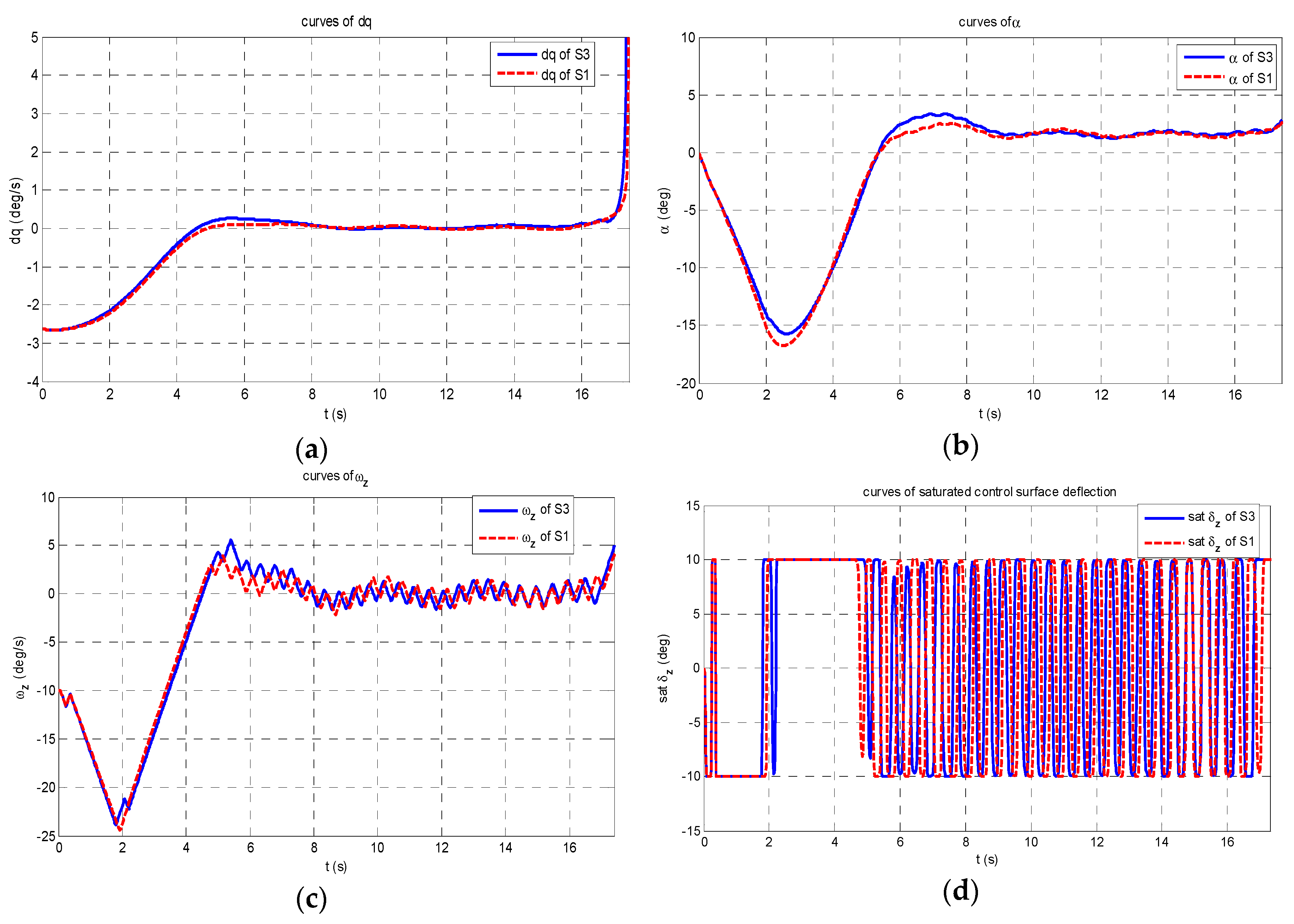
Figure 3 shows the comparison simulation results between S2 and S1. The proposed control scheme is able to cancel out influence of the nonlinear uncertainty in aerodynamics coefficients of lift and moment. Figure 4 shows the comparison simulation results between S3 and S1. The nonlinear parts of control surface deflection in aerodynamics coefficients have a limited impact on the convergence with small overshoot in Figure 4a,b. It is indicated that the performance improves under complex nonlinearity with the help of the great approximation ability of neural network.
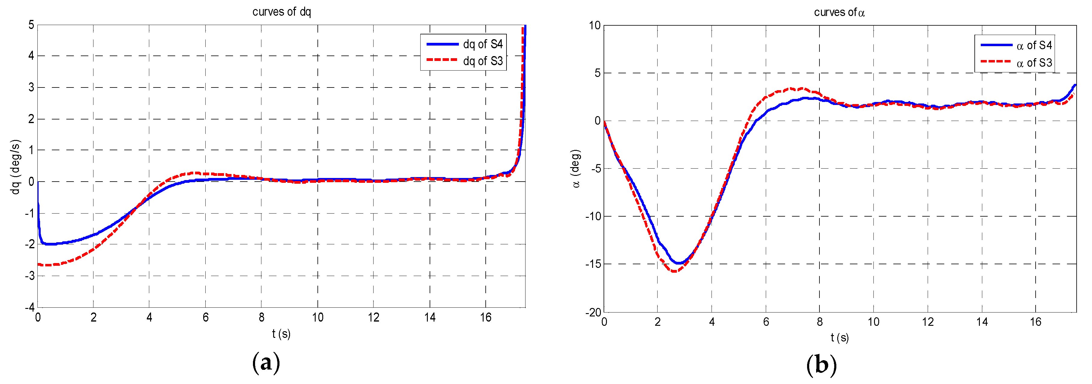
The comparison results of S3 and S4 are shown in Figure 5, which indicate that the proposed method can cancel out the complex uncertainties and disturbances with unknown measurement dynamics.
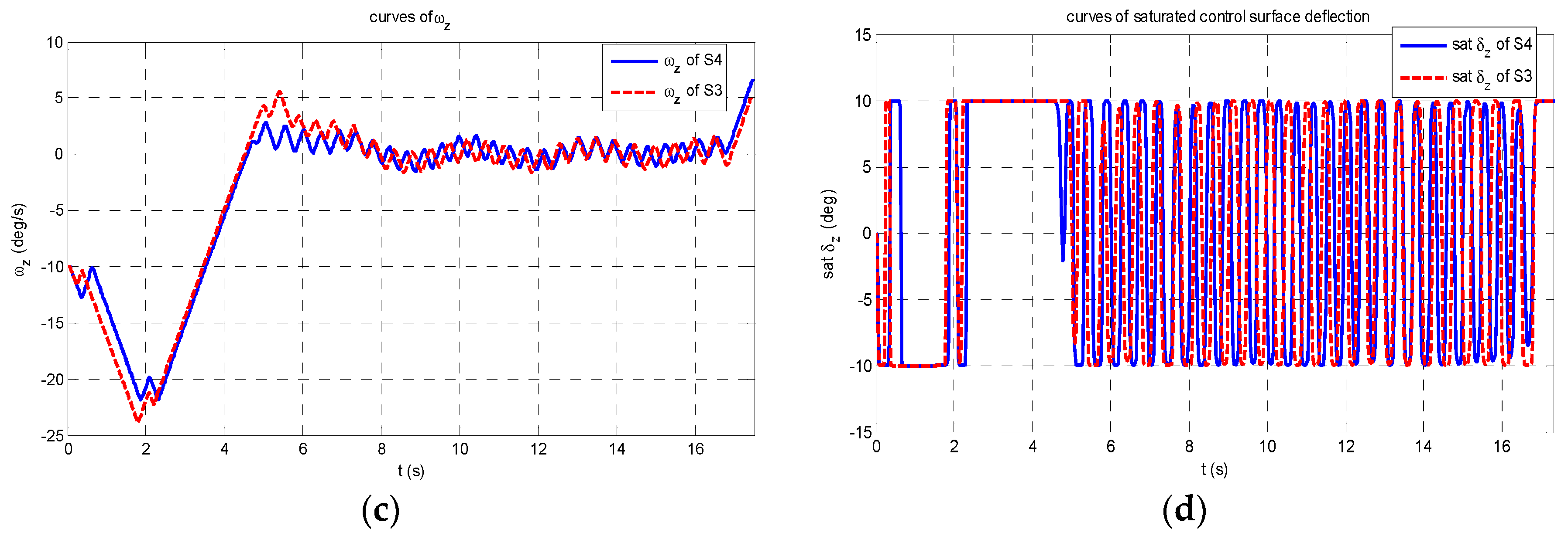
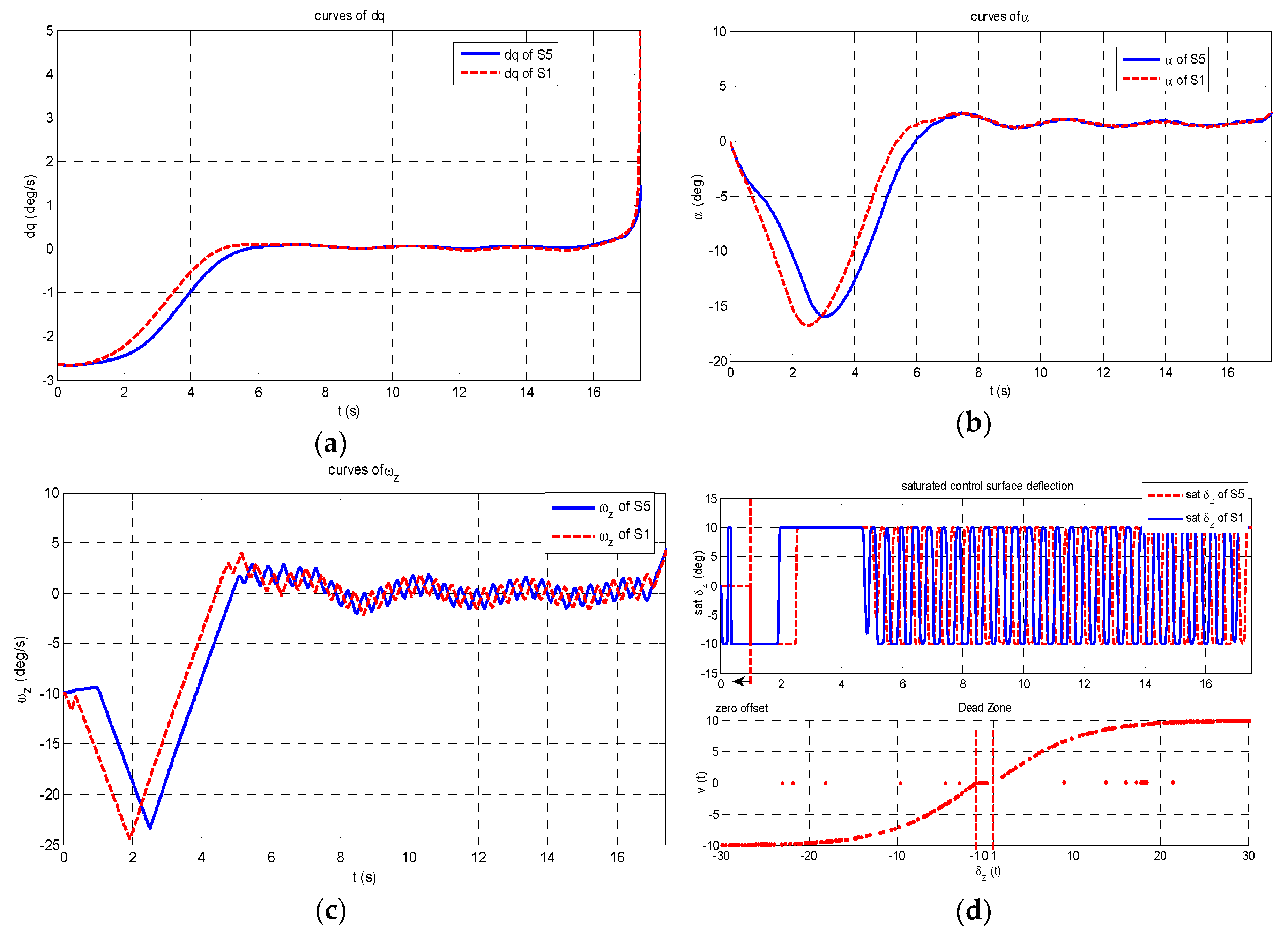
In Figure 6, simulation results in S1 and S5 are compared. Figure 5d shows that the control surface deflection of S5 has 1 deg dead-zone. It is seen that the NESO approximation-based IGC control scheme guarantees that the closed-loop system is stable under saturated control surface deflection with dead-zone nonlinearity.
6.3. Simulations with Velocity, Aerodynamics Coefficients Bias and Measurement Noises
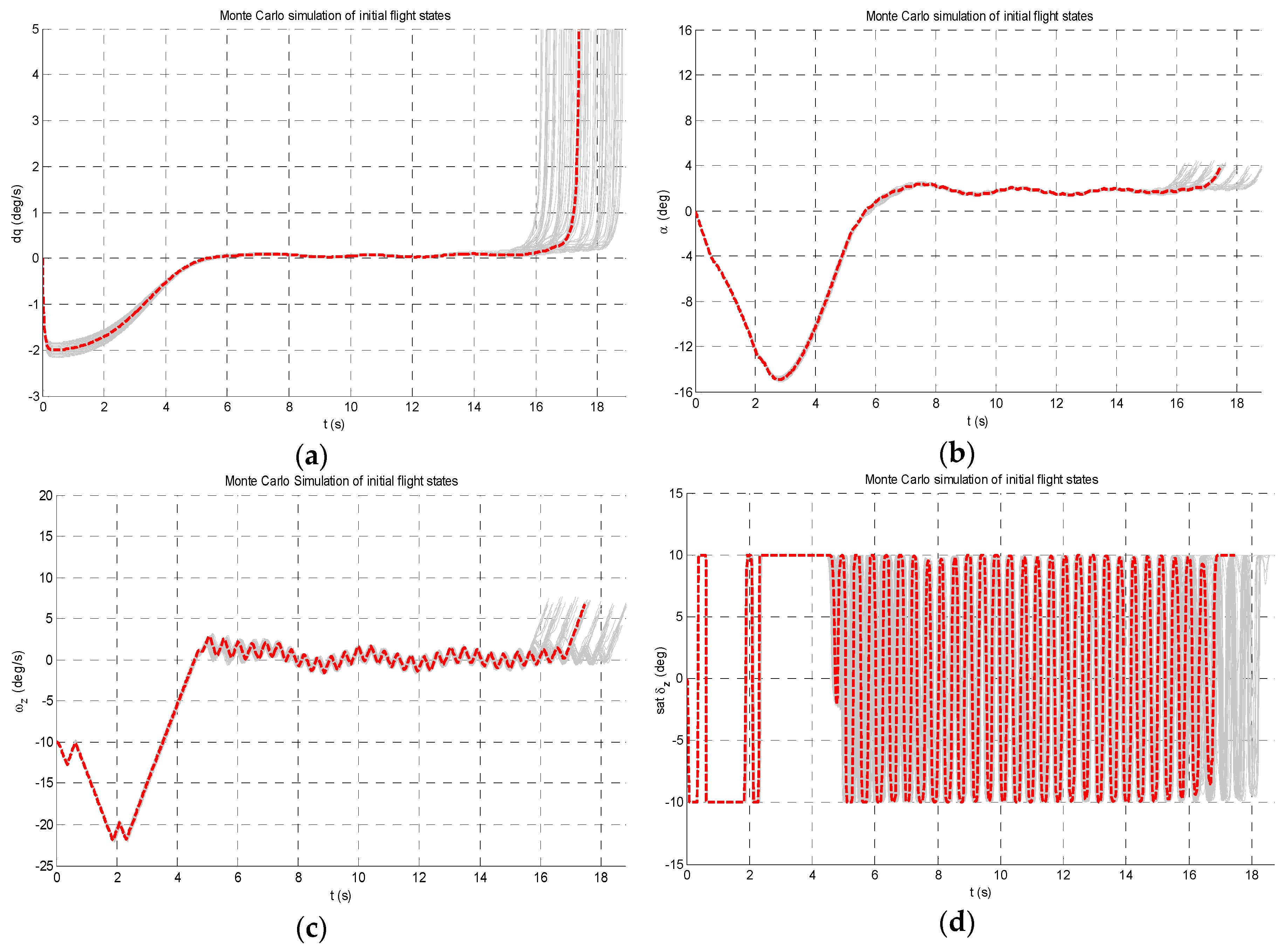
With the help of Monte Carlo theory, a large number of numerical simulations under large uncertainties of velocity, aerodynamics coefficients and measurement noises is made to test robustness of the proposed design. In Figure 7, the simulation results under velocity dispersion between 1000 m/s and 1400 m/s are presented. The mean value is 1200 m/s, and the red curves shows the corresponding results. It is seen that the parameter settings of the proposed controller can satisfy large variations of initial flight velocity.
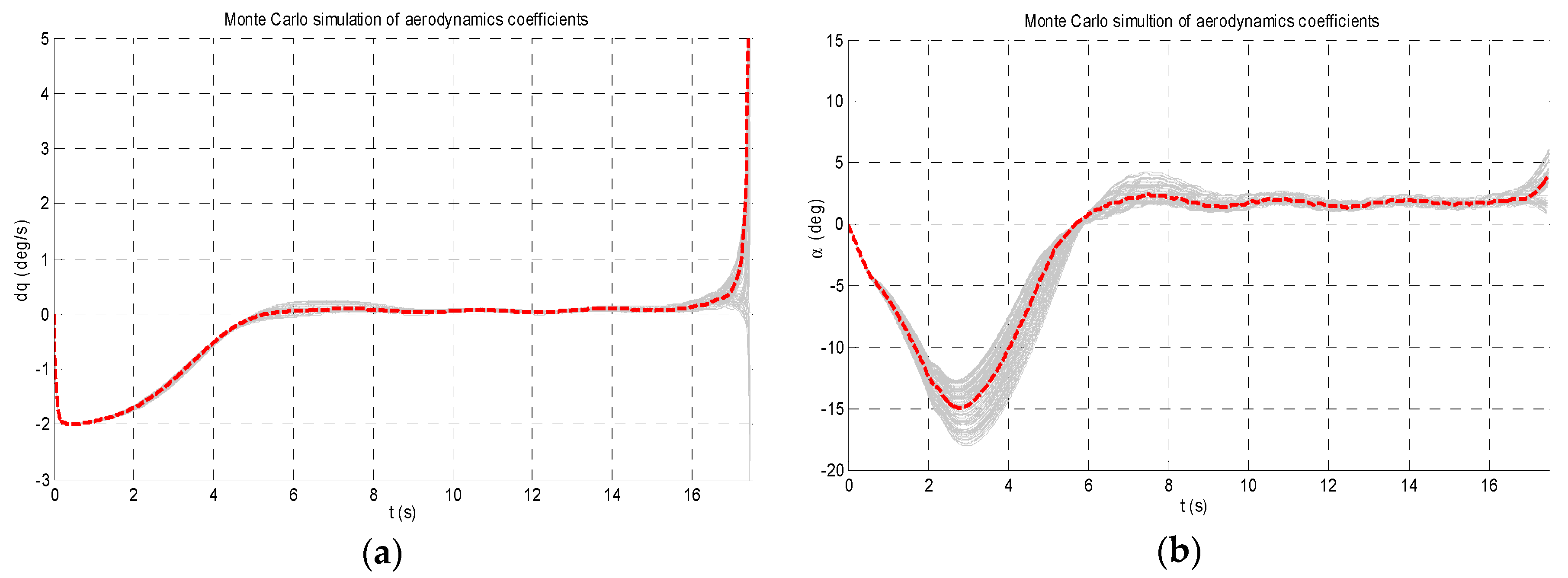
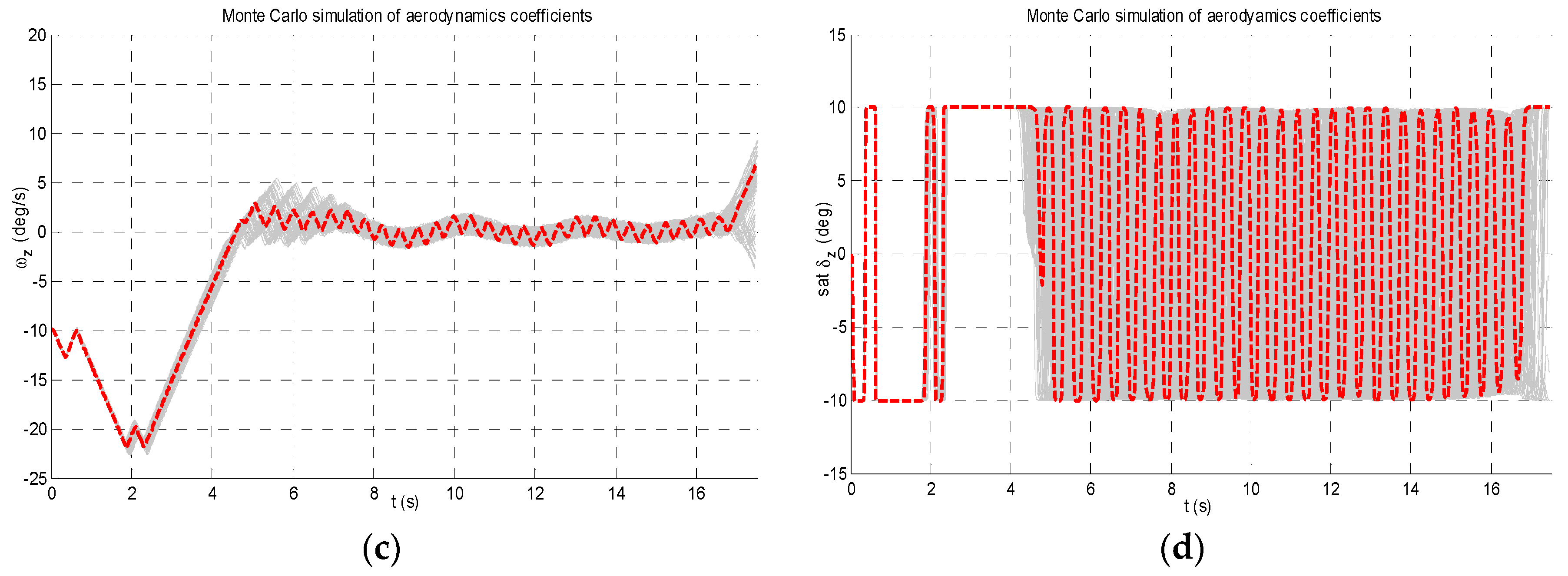
Figure 8 presents the Monte Carlo simulation results under aerodynamics coefficients bias with uncertainties in of S3. The results indicate that the proposed IGC scheme is able to cancel out the great aerodynamics uncertainties in hypersonic flight.
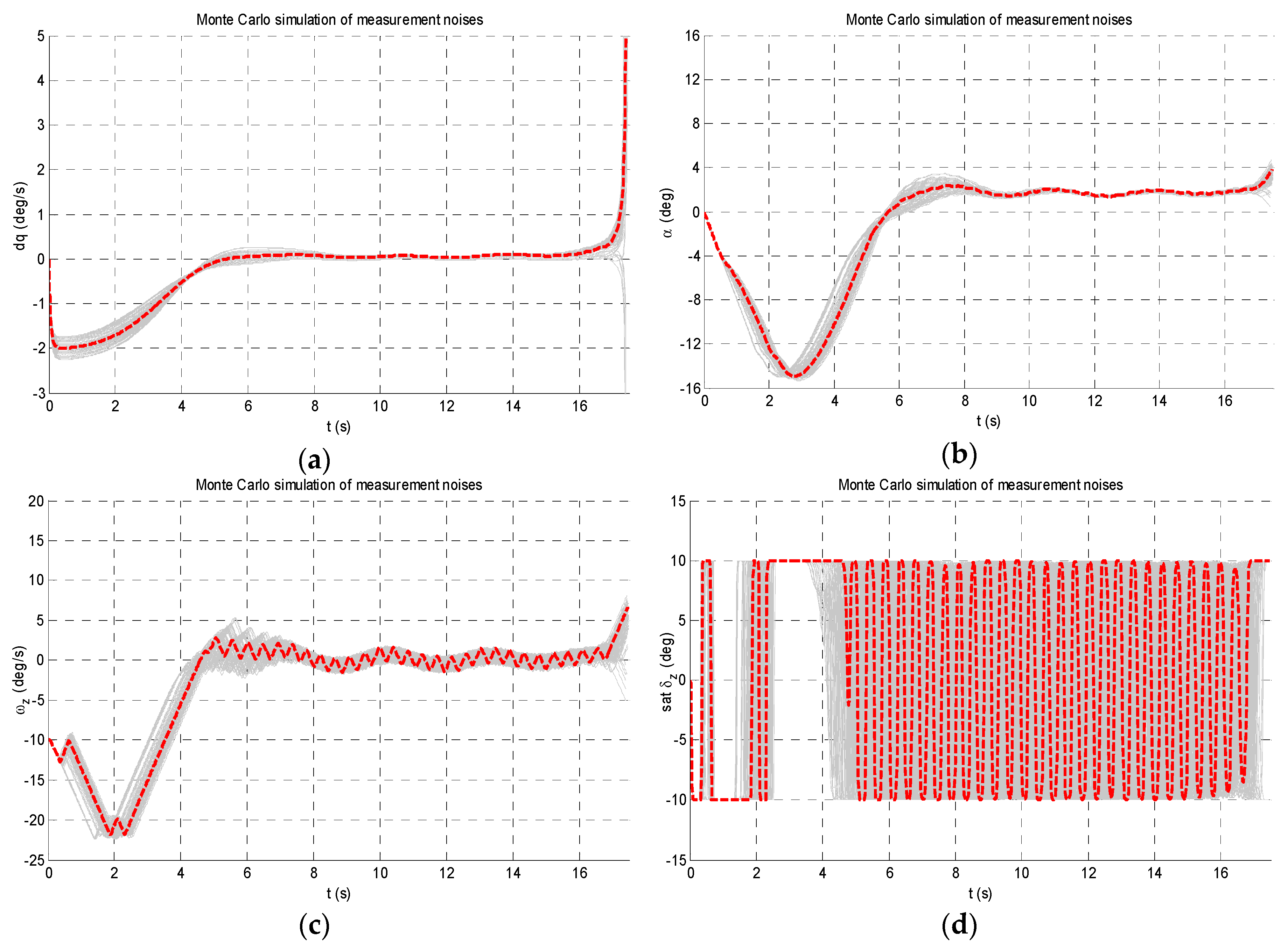
In Figure 9, the Monte Carlo simulation results under measurement noises with uncertainties in gain and time constant in Equation (40d) are presented. It can be concluded that the proposed controller has good robustness in the presence of large uncertainties of measurement dynamics.
7. Conclusions
A novel composite IGC scheme in the presence of high-order nonlinear actuator dynamics is developed to address nonlinear hypersonic flight control with control input constraint and multiple uncertainties. The complex aerodynamics uncertainties and time-varying disturbances in different channels are well estimated by extended state observers improved by neural networks. Hybrid differentiators are employed to avoid directly differentiating the virtual control inputs in the back-stepping process. Thus, the peaking phenomenon and chasing of back-stepping sliding mode controller is greatly depressed. Nussbaum function is introduced to deal with the unknown direction of saturated control surface deflection. Series of numerical simulations indicate that the NESO-based IGC scheme can cancel out large uncertainties and disturbances. In conclusion, the proposed approach extends IGC application in hypersonic flight more practically and efficiently.
Author Contributions
Conceptualization, L.W.; Methodology, L.W.; Software, L.W.; Validation, L.W., K.P. and W.Z.; Formal Analysis, L.W.; Data Curation, L.W.; Writing—Original Draft Preparation, L.W.; Writing—Review & Editing, L.W., K.P. and D.W.; Project Administration, K.P., W.Z. and D.W.
Funding
This research received no external funding.
Conflicts of Interest
The authors declare no conflict of interest.
Appendix A
The “hypersonic weapon” was conceived to be a carrier vehicle for penetrator warheads and any suitable weapons or submunitions already being developed for the aircraft community. Since the concept used a common aero shell, the decision was made to call the new weapon the Common Aero Vehicle (CAV). The same CAV would also be common to a large number of launch systems, including reusable launch vehicles (RLVs), expendable launch vehicles (ELVs), retired Inter-Continental Ballistic Missiles (ICBMs), and air launch from a variety of platforms. The aerodynamics of NASA CAV-L (CAV with low lift-drag ratio) in 1998 is outlined in the following table:
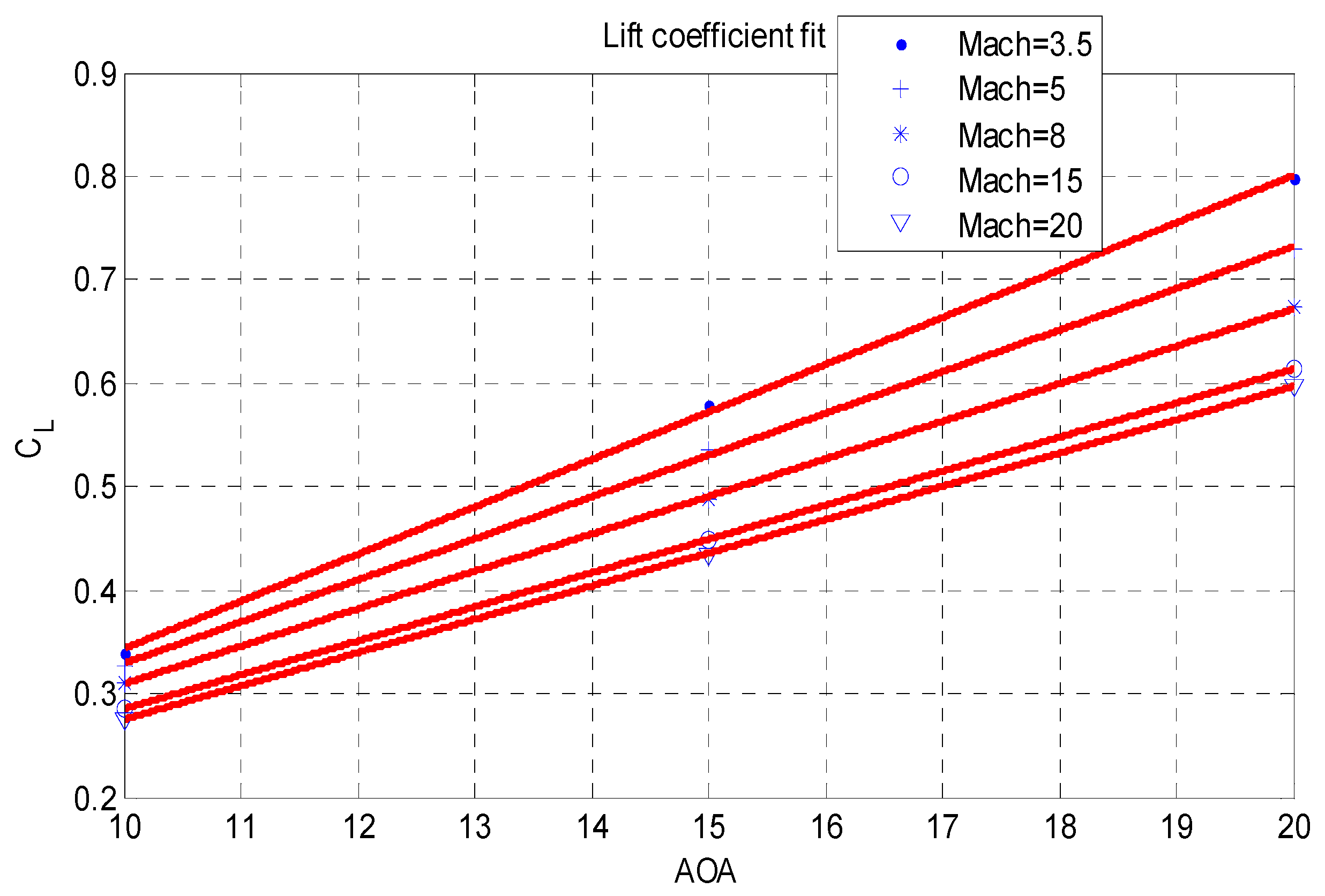
In hypersonic flight, the polynomial fit results of lift coefficient can be depicted as , which can be seen in Figure A1 and Table A1.

Table A1.
CAV-L Lift Coefficient ( ).
| AOA | Mach 3.5 | Mach 5 | Mach 8 | Mach 15 | Mach 20 | Mach 23 |
|---|---|---|---|---|---|---|
| 10 deg | 0.3401 | 0.3264 | 0.3108 | 0.2856 | 0.2760 | 0.2739 |
| 15 deg | 0.5786 | 0.5358 | 0.4883 | 0.4491 | 0.4349 | 0.4319 |
| 20 deg | 0.7975 | 0.7291 | 0.6731 | 0.6137 | 0.5975 | 0.5966 |
AOA: Angle of Attack. Mach: Mach number.
Figure A1.
Polynomial fit results.

References
- Schierman, J.D.; Ward, D.G.; Hull, J.R.; Gandhi, N.; Oppenheimer, M.; Doman, D.B. Integrated adaptive guidance and control for re-entry vehicles with flight test results. J. Guid. Control Dyn. 2004, 27, 975–986. [Google Scholar] [CrossRef]
- Shima, T.; Idan, M.; Colan, O.M. Sliding mode control for integrated missile autopilot guidance. J. Guid. Control Dyn. 2006, 29, 250–260. [Google Scholar] [CrossRef]
- Shima, T.; Idan, M.; Golan, O.M. Integrated sliding mode Autopilot-Guidance for Dual-Control Missiles. J. Guid. Control Dyn. 2007, 30, 1081–1089. [Google Scholar]
- Christian; Tournes, H.; Shtessel, Y.B. Integrated guidance and autopilot for dual controller missiles using higher order sliding mode controllers and observers. In Proceedings of the AIAA Guidance, Navigation and Control Conference and Exhibit, Honolulu, HI, USA, 18–21 August 2008. [Google Scholar]
- Harl, N.; Balakrishnan, S.N.; Phillips, C. Sliding mode integrated missile guidance and control. In Proceedings of the AIAA Guidance, Navigation, and Control Conference, Toronto, ON, Canada, 2–5 August 2010. [Google Scholar]
- Wang, J.; Liu, L.; Tang, G. Integrated guidance and control for hypersonic vehicles in dive phase with multiple constraints. Aerosp. Sci. Technol. 2016, 53, 103–115. [Google Scholar] [CrossRef]
- Zhang, C.; Wu, Y. Non-singular terminal dynamic surface control based integrated guidance and control design and simulation. ISA Trans. 2016, 63, 112–120. [Google Scholar]
- Wang, W.; Xiong, S.; Wang, S.; Song, S.; Lai, C. Three dimensional impact angle constrained integrated guidance and control for missiles with input saturation and actuator failure. Aerosp. Sci. Technol. 2016, 53, 169–187. [Google Scholar] [CrossRef]
- Liu, X.; Huang, W.; Du, L. An integrated guidance and control approach in three-dimensional space for hypersonic missile constrained by impact angles. ISA Trans. 2017, 66, 164–175. [Google Scholar] [CrossRef] [PubMed]
- Xia, Y.; Zhu, Z.; Fu, M. Back-stepping sliding mode control for missile systems based on an extended state observer. IET Control Theory Appl. 2009, 5, 93–1002. [Google Scholar] [CrossRef]
- Shao, X.; Wang, H. Back-stepping active disturbance rejection control design for integrated missile guidance and control system via reduced-order ESO. ISA Trans. 2015, 57, 10–22. [Google Scholar]
- Huang, J.; Ri, S.; Liu, L.; Wang, Y.; Kim, J.; Pak, G. Nonlinear disturbance observer-based dynamic surface control of mobile wheeled inverted pendulum. IEEE Trans. Control Syst. Technol. 2015, 23, 2400–2407. [Google Scholar] [CrossRef]
- Guo, Q.; Zhang, Y.; Celler, B.G.; Su, S.W. Back-stepping control of electro-hydraulic system based on extended-state-observer with plant dynamics largely unknown. IEEE Trans. Ind. Electron. 2016, 63, 6909–6919. [Google Scholar] [CrossRef]
- Park, J.; Sandberg, I.W. Universal approximation using radial basis function networks. Neural Comput. 1991, 3, 246–257. [Google Scholar] [CrossRef]
- Wu, Y.; Wang, H.; Zhang, B.; Du, K.L. Using radial basis function networks for function approximation and classification. Int. Sch. Res. Netw. Appl. Math. 2012, 2012, 1–34. [Google Scholar] [CrossRef]
- Bin, X. Robust adaptive neural control of flexible hypersonic flight vehicle with dead-zone input nonlinearity. Nonlinear Dyn. 2015, 80, 1509–1520. [Google Scholar]
- Wang, Y.; Wu, H. Adaptive robust backstepping control for a class of uncertain dynamical systems using neural networks. Nonlinear Dyn. 2015, 81, 1597–1610. [Google Scholar] [CrossRef]
- Chen, B.; Zhang, H. Observer based adaptive neural network control for nonlinear systems in nonstrict-feedback form. IEEE Trans. Neural Netw. Learn. Syst. 2016, 27, 89–98. [Google Scholar] [CrossRef] [PubMed]
- Bu, X.; Wu, X.; Wei, D.; Huang, J. Neural approximation based robust adaptive control of flexible air-breathing hypersonic vehicles with parametric uncertainties and control input constraints. Inf. Sci. 2016, 347, 29–43. [Google Scholar] [CrossRef]
- Wen, C.; Zhou, J.; Liu, Z.; Su, H. Robust adaptive control of uncertain nonlinear systems in the presence of input saturation and external disturbance. IEEE Trans. Autom. Control 2011, 56, 1672–1678. [Google Scholar] [CrossRef]
- Chen, C.; Liu, Z.; Zhang, Y.; Chen, C.P. Adaptive control of robotic systems with unknown actuator nonlinearities and control directions. Nonlinear Dyn. 2015, 81, 1289–1300. [Google Scholar] [CrossRef]
- Chen, C.; Liu, Z.; Zhang, Y.; Chen, C.P.; Xie, S. Saturated Nussbaum function based approach for robotic systems with unknown actuator dynamics. IEEE Trans. Cybern. 2016, 46, 2311–2321. [Google Scholar] [CrossRef] [PubMed]
- Farrell, J.A.; Polycarpou, M.; Sharma, M.; Dong, W. Command filtered backstepping. In Proceedings of the American Control Conference, Seattle, WA, USA, 11–13 June 2008. [Google Scholar]
- Hou, M.; Duan, G. Adaptive dynamic surface control for integrated missile guidance and autopilot. Int. J. Autom. Comput. 2011, 8, 122–127. [Google Scholar] [CrossRef]
- Liang, X.; Hou, M.; Duan, G. Adaptive dynamic surface control for integrated missile guidance autopilot in the presence of input saturation. J. Aerosp. Eng. 2014, 28, 0414121. [Google Scholar] [CrossRef]
- Pan, Y.; Yu, H. Dynamic surface control via singular perturbation analysis. Automatica 2015, 57, 19–33. [Google Scholar] [CrossRef]
- Xu, B.; Wang, S.; Gao, D.; Zhang, Y.; Shi, Z. Command filter based robust nonlinear control of hypersonic aircraft with magnitude constraints on states and actuators. J. Intell. Robot Syst. 2014, 73, 233–247. [Google Scholar] [CrossRef]
- Wang, L.; Zhang, W.; Wang, D.; Peng, K.; Yang, H. Command filtered back-stepping missile integrated guidance and autopilot based on extended state observer. Adv. Mech. Eng. 2017, 9, 1–13. [Google Scholar] [CrossRef]
Figure 1.
The planar geometry in terminal phase.

Figure 2.
States and estimate errors of S1: (a) comparison between and NESOI, (b) comparison between and NESOII, (c) comparison between and NESOIII, and (d) saturated curve.
Figure 2.
States and estimate errors of S1: (a) comparison between and NESOI, (b) comparison between and NESOII, (c) comparison between and NESOIII, and (d) saturated curve.


Figure 3.
Comparison between S1 and S2: (a) curves of , (b) curves of , (c) curves of , and (d) curves of saturated .
Figure 3.
Comparison between S1 and S2: (a) curves of , (b) curves of , (c) curves of , and (d) curves of saturated .

Figure 4.
Comparison between S1 and S3: (a) curves of , (b) curves of , (c) curves of , and (d) curves of saturated .
Figure 4.
Comparison between S1 and S3: (a) curves of , (b) curves of , (c) curves of , and (d) curves of saturated .

Figure 5.
Comparison between S3 and S4: (a) curves of , (b) curves of , (c) curves of , and (d) curves of saturated .
Figure 5.
Comparison between S3 and S4: (a) curves of , (b) curves of , (c) curves of , and (d) curves of saturated .


Figure 6.
Comparison between S1 and S5: (a) curves of , (b) curves of , (c) curves of , and (d) curves of saturated .
Figure 6.
Comparison between S1 and S5: (a) curves of , (b) curves of , (c) curves of , and (d) curves of saturated .

Figure 7.
Monte Carlo Simulation under dispersion: (a) curves of , (b) curves of , (c) curves of , and (d) curves of saturated .
Figure 7.
Monte Carlo Simulation under dispersion: (a) curves of , (b) curves of , (c) curves of , and (d) curves of saturated .

Figure 8.
Monte Carlo simulation under aerodynamics coefficients bias: (a) curves of , (b) curves of , (c) curves of , and (d) curves of saturated .
Figure 8.
Monte Carlo simulation under aerodynamics coefficients bias: (a) curves of , (b) curves of , (c) curves of , and (d) curves of saturated .


Figure 9.
Monte Carlo simulation under measurement noises: (a) curves of , (b) curves of , (c) curves of , and (d) curves of saturated .
Figure 9.
Monte Carlo simulation under measurement noises: (a) curves of , (b) curves of , (c) curves of , and (d) curves of saturated .

© 2018 by the authors. Licensee MDPI, Basel, Switzerland. This article is an open access article distributed under the terms and conditions of the Creative Commons Attribution (CC BY) license (http://creativecommons.org/licenses/by/4.0/).
Share and Cite
MDPI and ACS Style
Wang, L.; Peng, K.; Zhang, W.; Wang, D. Neural Extended State Observer Based Intelligent Integrated Guidance and Control for Hypersonic Flight. Energies 2018, 11, 2605. https://doi.org/10.3390/en11102605
AMA Style
Wang L, Peng K, Zhang W, Wang D. Neural Extended State Observer Based Intelligent Integrated Guidance and Control for Hypersonic Flight. Energies. 2018; 11(10):2605. https://doi.org/10.3390/en11102605
Chicago/Turabian StyleWang, Liang, Ke Peng, Weihua Zhang, and Donghui Wang. 2018. "Neural Extended State Observer Based Intelligent Integrated Guidance and Control for Hypersonic Flight" Energies 11, no. 10: 2605. https://doi.org/10.3390/en11102605
Note that from the first issue of 2016, this journal uses article numbers instead of page numbers. See further details here.