Reserve Allocation of Photovoltaic Systems to Improve Frequency Stability in Hybrid Power Systems


1
Department of Electrical Engineering and Automation, Aalto University, 02150 Espoo, Finland
2
Faculty of Electrical and Computer Engineering, Babol (Noshirvani) University of Technology, Babol PO Box 484, Iran
3
ABB 54 Export Drive, Darwin Business Park, Darwin 0828, Australia
4
C-MAST, University of Beira Interior, R. Fonte do Lameiro, 6201-001 Covilhã, Portugal
*
Author to whom correspondence should be addressed.
Energies 2018, 11(10), 2583; https://doi.org/10.3390/en11102583
Submission received: 15 September 2018
/
Revised: 19 September 2018
/
Accepted: 25 September 2018
/
Published: 27 September 2018
(This article belongs to the Section F: Electrical Engineering)
Abstract
:This study suggests a model to include a solar power system or photovoltaic system (PV) in the control of frequency by taking into account a percentage of the PV power production for back-up reserve. This is done by investigating two scenarios: PV contribution in (1) initial primary frequency control and (2) entire primary frequency control. As explained in section three, 10% power of the PV modules which receive more than 400 w/m2 irradiation is allocated for the power reserve. The power generation of photovoltaic systems depends largely on weather conditions which makes their output power associated with some degree of uncertainty. For this reason, in this paper, a PV system is considered along with conventional hydro and thermal units and they are modeled in MATLAB/Simulink (version 9.3, MathWorks, Natick, MA, USA) with the purpose of exploring the behavior of the intended method. In the next phase, for further studies, this system is extended to multi-area power systems including gas turbines. The results of the simulation demonstrated that the photovoltaic involvement in the control of frequency can successfully amend the frequency of the overall network. Not only it can decrease the overshoot and undershoot of the frequency response, it has the ability to improve the settling time as well, which helps the system reach the steady state easily and in shorter time. Specifically, the overshoot has reached nearly zero in both one area and two area systems and undershoot has declined up to 60% and 50% in the one area and two-area system, respectively. Considering settling time, while it had a negligible improvement in the one area system, it showed a remarkable enhancement in the two-area system, which improved from about 25 s to 6 s by using the proposed method.
1. Introduction
The disparity amongst the load demand and the generated power in power grids is a cause of variations of frequency and power interchange among distinct parts. The load frequency control (LFC) is usually recognized as a solution for the phenomenon of imbalance in the active power of the power grid [1]. Generally, LFC acts to retrieve the frequency of the system and the exchanging power to their projected value [2,3]. Recently, the power system has increased in size and complexity which imposes the requirement for intelligent control systems to manage a diverse range of energy resources, including the flourishing renewable energies. The solar energy harnessed through PV systems is becoming one of the most advantageous renewable energy resources (RERs) thanks to benefits such as being abundant, environmentally friendly, having modular structure, having a low cost of operation and maintenance, and an absence of noise which makes it a fitting technology for urban areas. However, the uncertainty due to the variability in their power generation is causing an increased mismatch between the generated power and the load. This property results in continuous deviations from the nominal frequency, so a more effective frequency control in the service is required [4,5]. Moreover, maximum power point tracking algorithms are typically used by PV systems with the aim of generating the highest probable power in situations where PV systems are connected to the grid. Such a feature is quite useful for exploiting the most out of the resources. However, it does not seem to be very effective for the control of the frequency or load tracking, particularly in microgrids. Such a condition could be even less desirable in microgrids comprised of mixed types of resources of renewable energy, leading to a situation in which ancillary regulation is required [6,7]. On that basis, and with the constant growing inclusion of PVs into the grid, it will be vital for these systems to deliver a certain level of support to the system stability, as has been traditionally provided by conventional rotating generators.
This subject has attracted the attention of many researchers. An energy regulation approach using an adaptive droop control methodology is offered in Ref. [8] for a PV–battery hybrid unit in a case study where the microgrid was isolated from the main grid. This hybrid system is configured to share the load demand with other generation units and store any extra generated power in the battery. In Ref. [9], a decentralized power management method is suggested in a PV-battery system which is installed in a droop-based controlled micro grid using the suggested multi-segment P/f representative bends for each system regardless of the internal communication and the central management algorithm. With the intention of reaching a balance for the power in the microgrid, the battery’s state of charge (SoC) and the accessible PV power are used to adjust these curves, locally and in real time, and coordinating the operation of such types of units independently. Although batteries facilitate renewable integration into grids, the capital and maintenance costs for battery energy storage (ES) is a challenge for large-scale PV system deployment. In Ref. [10], a numerical model is presented to have a better analysis of the PV performance. This study could lead to higher efficiency and longer lifetime besides enhancing the generated power forecast. Authors in Ref. [11] suggest a predictive PV control methodology with the aim of controlling the active power rapidly and precisely. The main contribution of this work is reducing frequency contingency events without using energy storage system. In Ref. [12], an adaptive-predictor-corrector-based tracking algorithm is suggested for a smart energy management system which is able to regulate the frequency without needing any storage system. This method is applied on a microgrid consisting of a diesel generator, PV array, and a fuel cell. In Ref. [13], a decentralized energy management approach based on a droop control is suggested for a hybrid PV and battery to make the PV system follow power and voltage references. In order to investigate the performance of the recommended system, a 3.5 kVA microgrid is considered for experimental purposes. In Ref. [14], a hybrid microgrid consisting of a PV system, hydro power, and a battery is considered for study and then frequency and voltage regulation are done by means of a bidirectional DC–DC converter. This is possible by absorbing the fluctuation of load demand by battery and regulating the DC bus voltage. Reference [15] investigated the frequency regulation issue in a medium-range voltage distribution network which is highly penetrated by the PV system. This is done by smart inverters which imitate the governor behavior in the traditional synchronous generators and don’t need any communication link. The proposed scheme in Ref. [16] presents decentralized active and reactive power control in a grid-tied smart PV inverter system while considering a power grid with a high penetration of PV. However, the requirement for communication infrastructure makes it a bit less desirable due to imposing additional cost on the whole system. In Ref. [17], the authors propose an online calculation method to enable PV work at a de-loaded margin in order to contribute to the frequency control of an isolated power network. The amount of de-loaded margin is adjustable, which determines the capacity for power reservation. The greater de-loaded margin results in a greater capability for frequency regulation but reduces the economic operation which occurs at the maximum power point of PV systems.
Allowing the PV to control active power by considering the maximum power tracking was an approach proposed in Ref. [18]. This active power control is performed by putting the voltage PV reference (VPV, ref) far from the voltage of MPP which is indicated by VMPP. In Ref. [19], a big PV-diesel system is considered and frequency control based on a fuzzy technique is presented for it. The power reference for a battery-PV inverter is specified by means of fuzzy reasoning that needs three items as input, including change of insolation, the medium of insolation, and frequency deviation. This method provides a decent control scheme, however, implementing and using a fuzzy logic controller has its own complexity where there is a need to define new fuzzy reasoning for any change in the system, such as increasing the PV power. In Ref. [20] a minimal-order observer-based control technique is suggested for a several PV systems in order to decrease frequency deviation. Two subsequent steps are needed to find the set points of the PV’s power. However, the practical implementation of the suggested control system is difficult and needs a rapid communication system, a data collection center, and a central control section.
Multiple PVs and controllable loads under a centralized control method formed a virtual power plant (VPP) in Ref. [21]. The demand of the controllable loads and the PV systems’ power output are organized by resolving a mixed integer programming (MIP) problem to flexibly adjust the VPP power production. Nevertheless, this methodology suffers from high complexity and by being time-consuming and may lead to failure since it uses two iterative algorithms, one depending on the other. In Ref. [22] a pseudo power point tracking method is introduced to provide a functionality of frequency regulation for PV systems. Through such a method, the raw produced power of the PV panel is traced by utilizing different processes embedded within an maximum power point (MPP) controller. For the true MPP, a Perturb and Observe algorithm is utilized and for the pseudo MPP, the open-circuit voltage algorithm is used. The Perturb and Observe algorithm is not very accurate and can fail under rapidly changing atmospheric conditions. In addition, the paper does not address how to specify constantly changing VOC while the system is in operation.
In this work, a novel regulation method is offered for PV systems in order to assist the control of frequency by reserving a portion of the produced power and allocating it to the frequency support. Initially, the maximum power is assessed through the means of an algorithm that uses particle swarm optimization (PSO) [19]. Consequently, a share of the aforementioned power is calculated and committed to the power reserve in order to be supplied into the grid whenever it is needed. Generally, connecting PVs that have strong power generation introduces pronounced technical challenges for the power grid since its intrinsic intermittent and fluctuant output characteristics will require an increase in the allocation of the spinning reserve by different non-renewable power generation resources. However, the main contribution while utilizing the proposed method is that the power reserve required by the system could be broadly decreased and it could also reduce the overall pressure on the conventional units of power generation and the capital and operation costs of the entire system. In addition, if used in an islanded microgrid, such a method could increase the stability and could efficiently mitigate the need for ES devices.
The rest of this paper is organized as follows. The description of the system under study is presented in Section 2 and the contribution of the PV system to frequency control is explained in Section 3. Section 4 describes the proposed controller and objective function and contains the simulation result for a one-area power system. The aim of Section 5 is to further study the suggested method by considering two-area power system and evaluating the performance of the proposed approach. Finally, the paper is concluded in Section 6.
2. System under Study
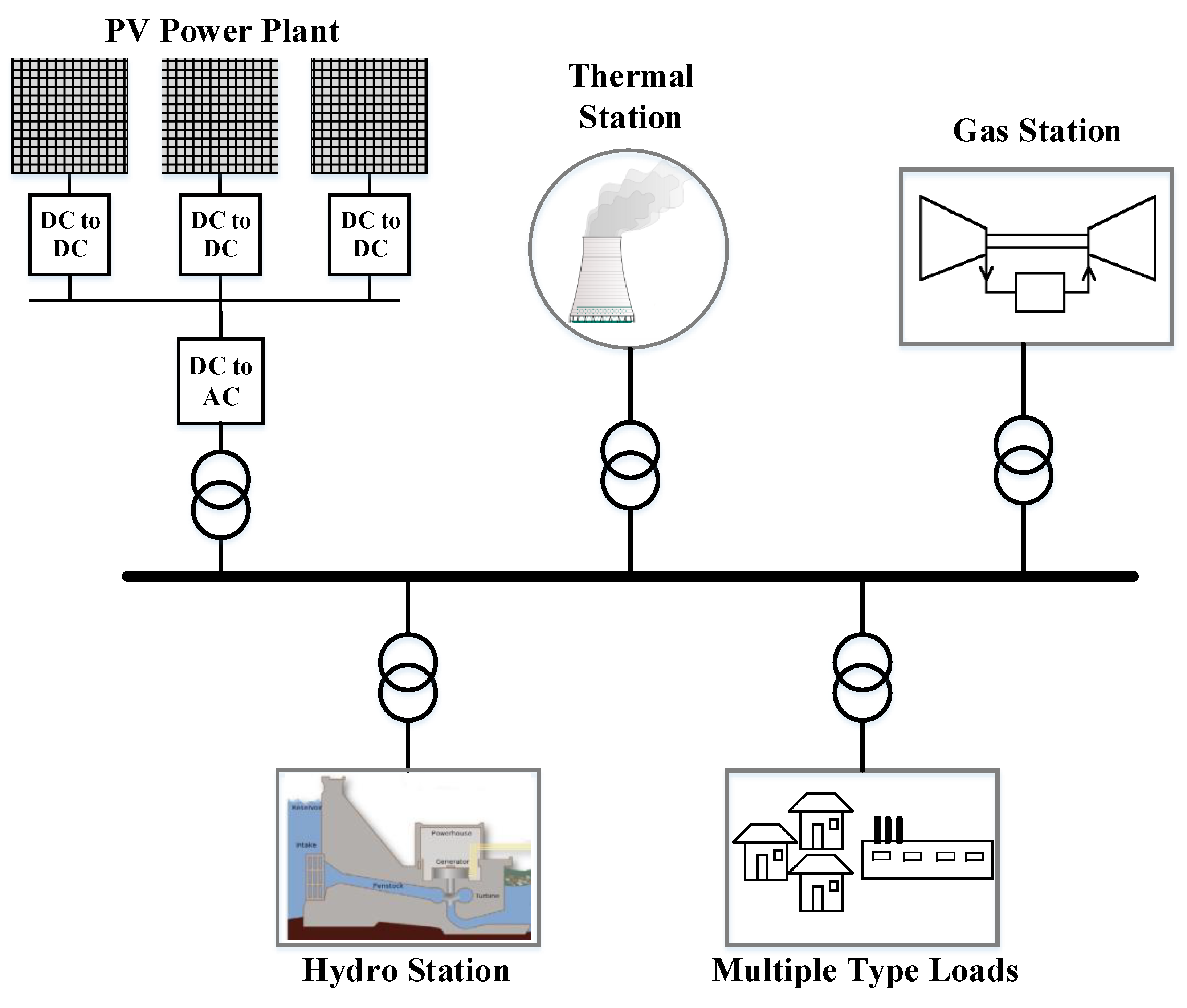
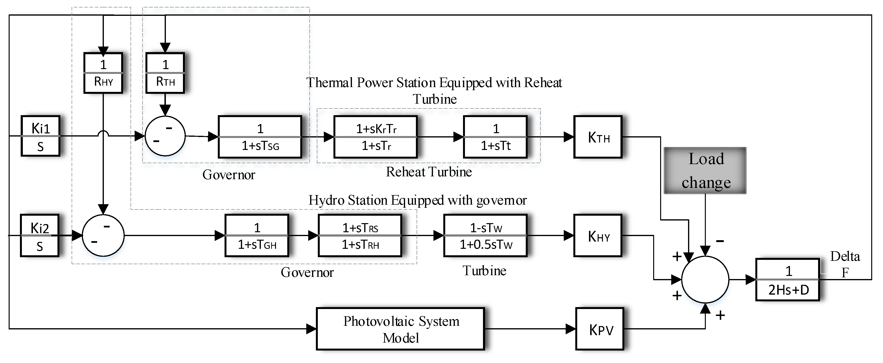
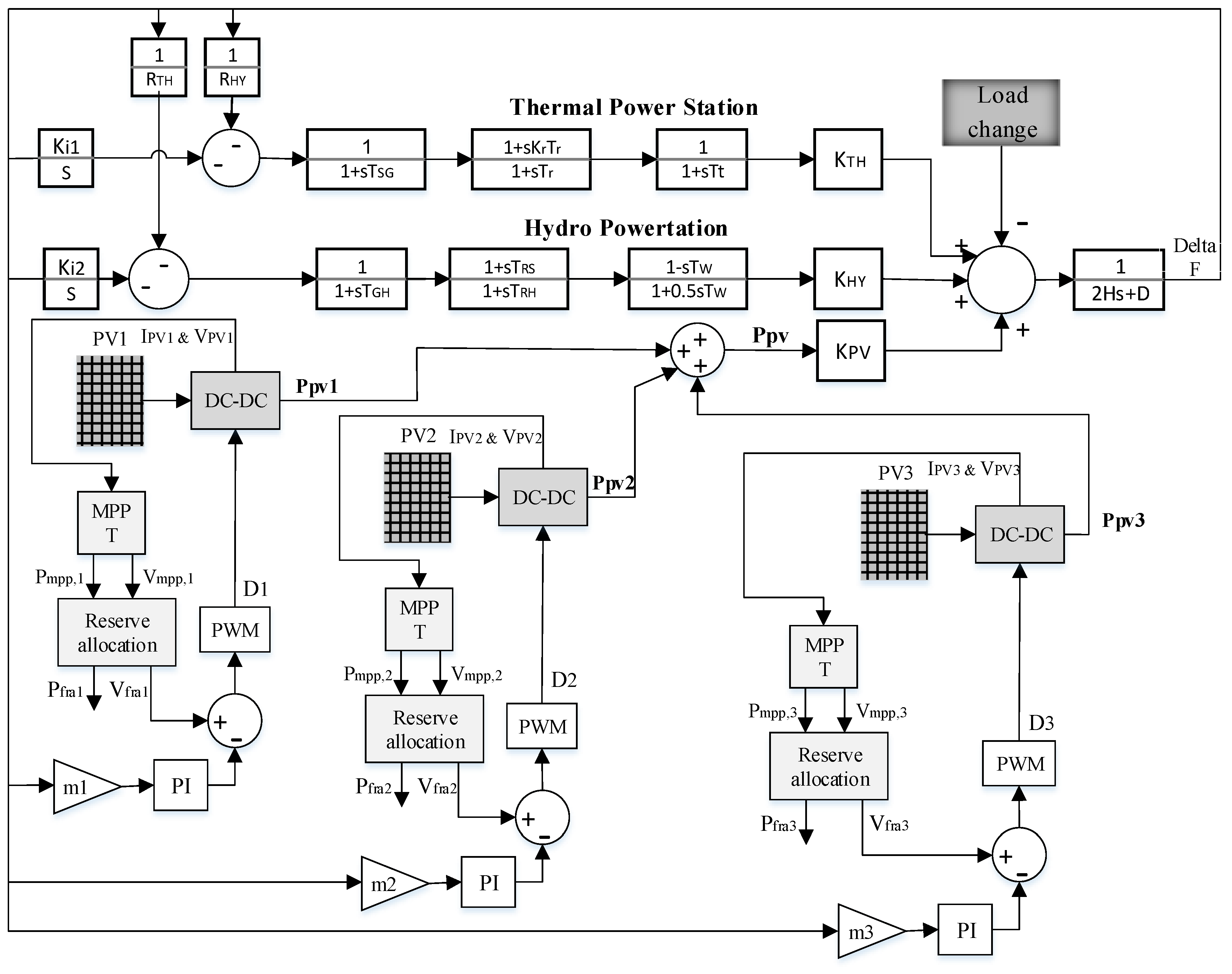
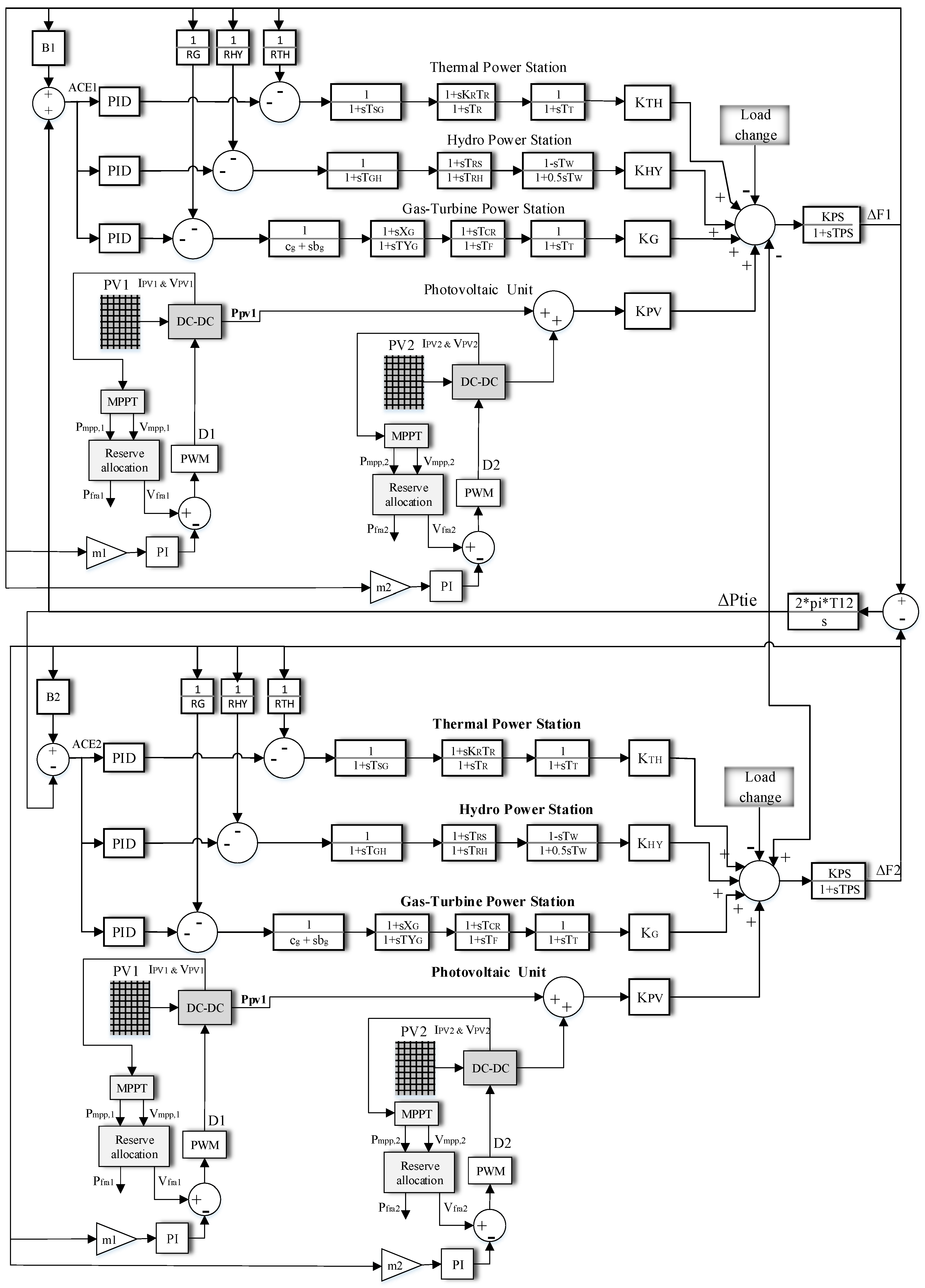
The focus of this work relies on a one-region power network comprising a hydro, thermal, and gas unit combined with a PV system which is shown in Figure 1. A linear model of the entire system for the purpose of LFC study and simulation is illustrated in Figure 2. The model of the hydro and thermal units is deduced from Ref. [23,24,25,26], and the model of the PV system with a contribution into the control of the frequency is addressed in Section 3.2.
The contribution factor for every single unit is taken into account separately in order to identify the participation of every individual plant to the whole loading. KHY, KPV, and KTH are the hydro, PV, and thermal unit factors of participation, correspondingly. These contribution factors sum to one. In Appendix A, the remaining system parameters can be found.
3. The Contribution of PV in the Control of Frequency
3.1. The Control of Frequency
As a general rule, three subcategories categorize the LFC elements. The primary control (circa a small number of milli-seconds), the secondary control (close to a few seconds), and tertiary control (from a few seconds to some minutes) [27]. Speed control of governor of generators and the inertia response are a part of the primary frequency control. The inertia acts relatively quickly, in less than half a second, right after immediate first response of the load sharing based on the generation connecting impedance. The difference is considerably more tangible for a frequency response by converters, as considered in this study, due to the fact that these converters mimick real inertia of rotors through variable synthetic inertia which makes them more influential compared to governor’s response [28].
The secondary control level is managed by controllers sitting on top of primary controllers and communicates data in order to allow each generation unit in order to adjust both its active and reactive power in harmony with the rest of online units. This is coordinated based on frequency and voltage setpoint signals sent from secondary controllers through primary controllers [29]. Based on the selected frequency, voltage control methods, and power sharing mechanisms, the setpoints are calculated and communicated with a larger time constant. The rotating generators reach completion of such a process in several seconds, while the control of the frequency based on converters have a generally quick response, typically less than a second. In addition, tertiary control modules usually consist of slow and long-term coordinating algorithms, such as Scheduling.
3.2. Evaluation of PV Contribution for the Control of Frequency
The power-frequency droop control in a typical grid is utilized for controlling the primary and secondary frequency. In this case, the entire systems’ frequency increases as a reaction to the excess power generation or shortage of the load demand and the vice versa [30,31]. For current grids characterized by higher penetration of PVs, the frequency can be compensated with the considered method in cases such as decreasing generation or increasing load that requires reserve power. Employing such a method is useful in at least two of the subsequent scenarios [18].
3.2.1. PV Deployment in Island Microgrids
Uncertainty and stability problems in remote islanded microgrids are caused by the variability of the power generation by RERs, which are incapable to export or import power from the nearby networks [19]. A potential solution is to employ a battery ES along with PV systems [32,33,34]. However, this means a significant increase in investment and maintenance costs [35]. Utilizing PV systems for frequency regulation allows reducing the size of the required ES device and it can also result in lower charging and recharging cycles of the battery ES [19]. Thus, this allows extension of the life span of the battery ES [36]. A proper allocation of PV capacity to frequency support can eliminate the requirement for the battery energy storage system (BESS) entirely, which reduces overall system cost substantially.
3.2.2. Networks Characterized by High Levels of PV Contribution
In cases in which the PV penetration rises in a large power network, the condition for the frequency regulation being covered by the ancillary service would be higher [37,38]. In these situations, the reserve power of conventional power plants needs to be raised in the grid in order to compensate for the fluctuation of PV systems which results in higher capital and fuel cost and more stress on the generation units.
3.3. Reserve Allocation of PV Modules to Contribute to Frequency Control
Usually, the PV modules are linked to the power system by combining an inverter, a boost converter, and a coupling transformer [39,40,41,42]. With the aim of getting the highest possible generated power from the PVs, it is essential to utilize maximum power point tracking (MPPT) algorithms that can achieve the goal by changing the boost converter duty cycle. For obtaining the available maximum power, a particle swarm optimization (PSO)-based algorithm is utilized in this paper [43].
3.3.1. Particle Swarm Optimization
The computational method, PSO, is a stochastic population-based optimization method introduced by Dr. Eberhart and Dr. Kennedy and it draws inspiration from the fish or bird’s social behavior [19]. It was introduced after social behavior investigation of organisms’ movements in a bird flock or fish school and was shaped based on the outcomes. For PSO, every bird has the name of a particle and is represented with a vector that is a potential solution [44,45]. By using this method, the possible solutions in the interior of the search space are randomly selected [46]. Consequently, the particles have a tendency to move in the direction of the best possible solution over the searching process. Considering a group of particles starts from the random vector in a specific range, and the velocity in the range of where is:
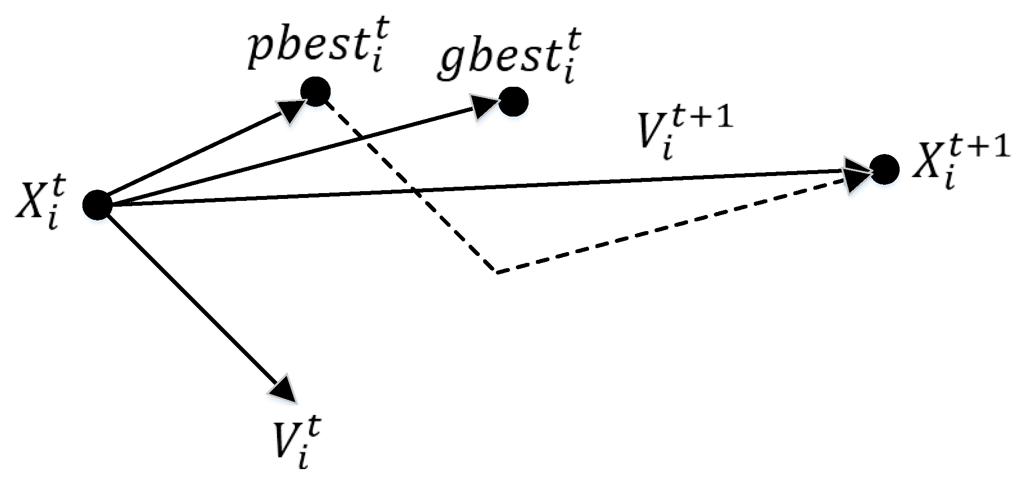
An objective function is established with the purpose of finding if the particle is near or not to the optimal solution. Every particle upholds the two best positions that are occupied. One of the aforementioned particles is that has experienced so far and the other is , representing the best solution practiced by all particles. In addition, the particles’ vectors are updated frequently by Equations (2) and (3) according to Figure 3. The updated population is the particle that is closer to the optimal solution. controls the speed of the next iteration and it is called the inertia weight. Larger leads to a more effective global search while smaller leads to a more efficient local search. (which are limited between 0 and 2) act as factors that conduct the search to local or social areas. Finally, represent generated numbers that are distributed uniformly in the range of and the iteration number is given by t.
This algorithm is quite advantageous due to the fact that is has a great efficiency and it has the capability to perform the MPPT in situations when the sky is partly clouded.
3.3.2. Reserve Allocation for the PVs
Once the assessment of the maximum feasible power for every PV module has been performed, in order to allow a contribution to frequency control, it is necessary to keep a portion of their power as reserve and to allocate it to this goal. In this proposal, 10% of the power generated from every PV module that receives irradiation greater than 400 w/m2 is assigned to the power reserve according to following equations:
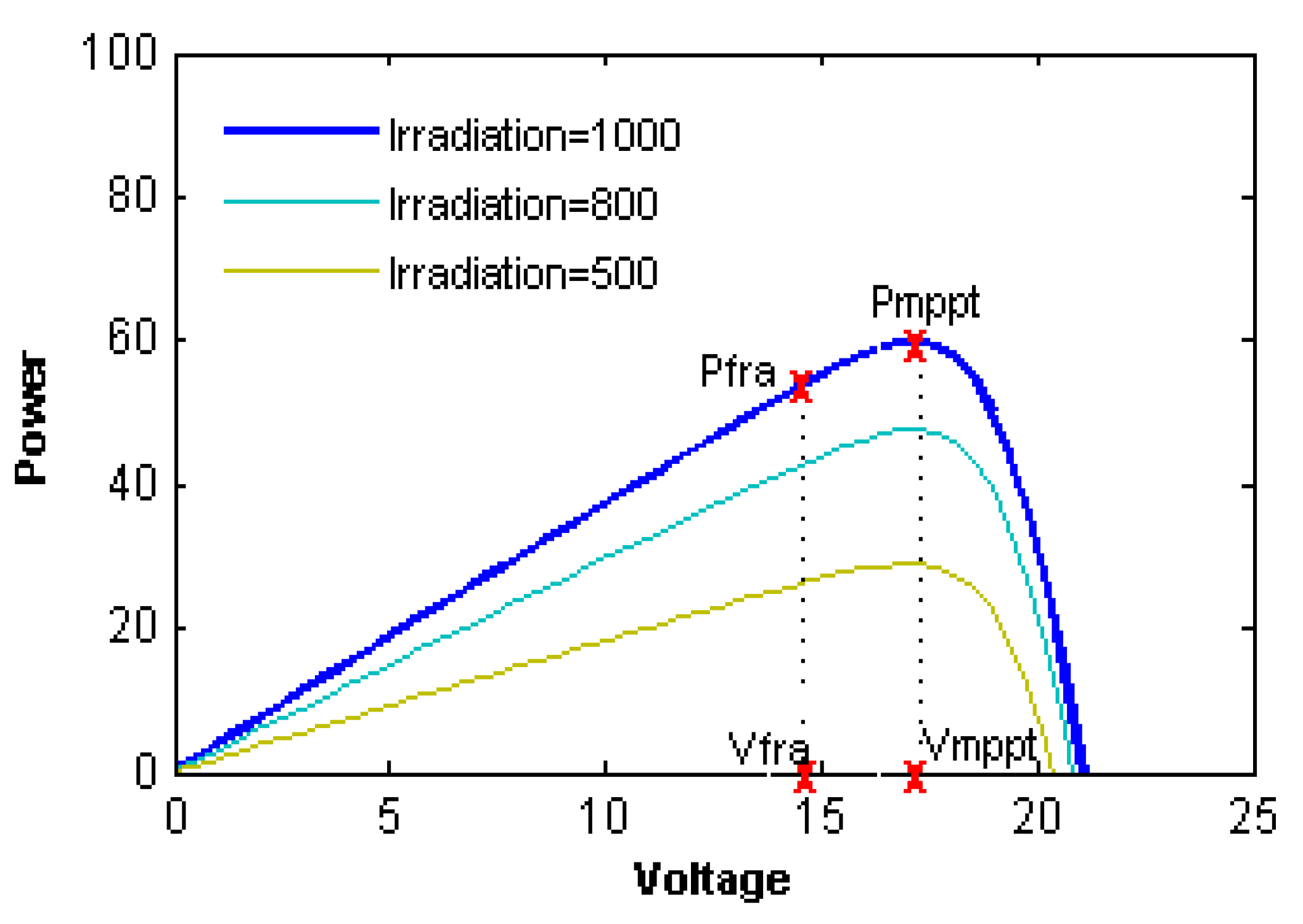
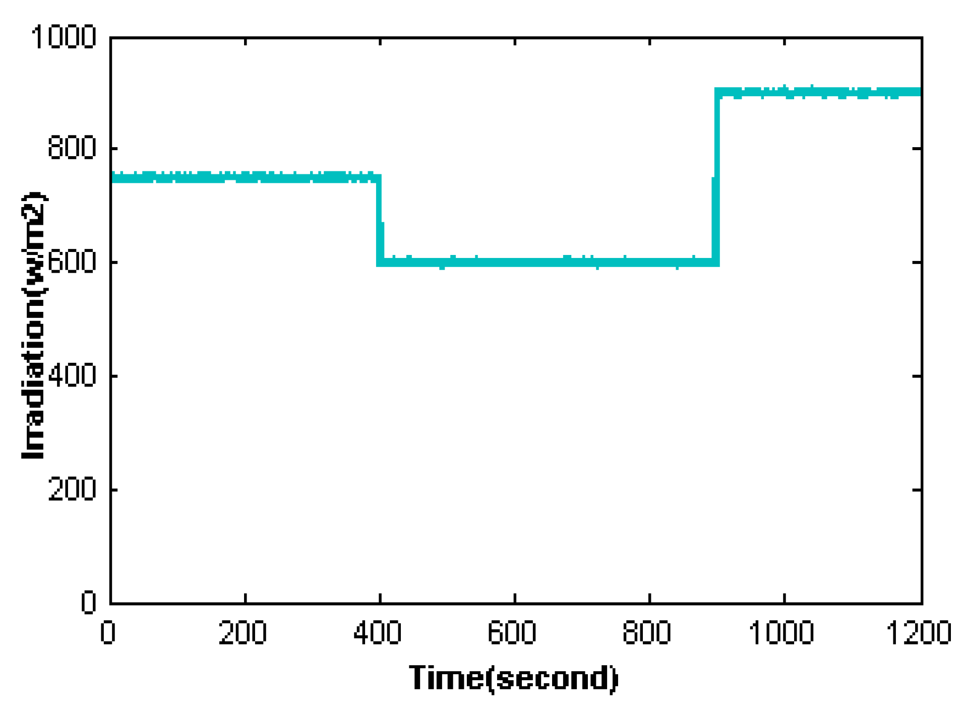
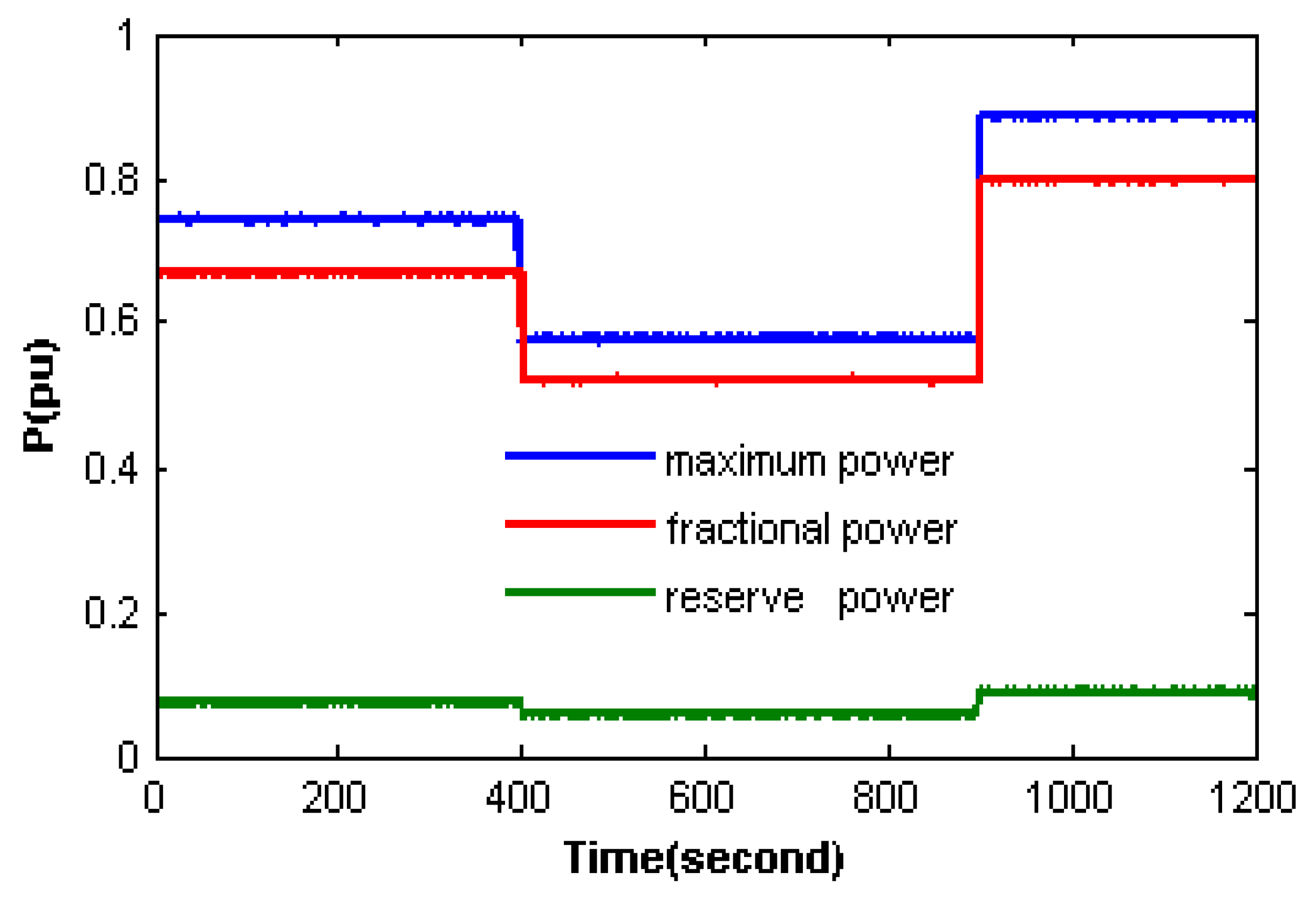
With the intention of assigning a part of the power generated by PVs into the reserve, it is vital to take into account aspects that have an effect on the PV-generated power. As a consequence, the PV module power relies upon three factors: output current (or voltage), irradiation, and temperature. In cases in which it is assumed that irradiation and temperature are constant, the power of the PV modules can be changed by alternating the PV’s voltage at the output terminal. Initially, the voltage () at which maximum power () occurs is quantified by the PSO. Later, reserve power for every module is given by mathematical expression 4 and the modules are required to operate at instead of. Therefore, the converters’ duty cycle of is changed so that is achieved as the boost converter’s output voltage instead of. In this way, whenever it is needed, the PV can raise its power from to by raising its output voltage from to. The power–voltage curve of a well-known PV module BP MSX 60 (Solar Electric Supply Inc., Scotts Valley, CA, US) is depicted in Figure 4. In case of irradiation identical to 1000 w/m2, the module’s maximum power is equal to 60 W and happens at 7.1 V. However, if the module’s voltage is set at 14.6 V, the power of the module ends at 54 W. Consequently, 6 W can be reserved by employing this approach, which is 10% of the generated power. In Figure 4, an example of a PV module with different irradiations over a period of twenty minutes is presented. , , and during this period are represented as per unit in Figure 5.
By observing this figure, 10% of the power produced by the aforementioned PV module will go to the reserve over the same period of twenty minutes.
With the PV modules reacting to the reduction of frequency, in line with Equation (7), their voltages change after identifying the fractional voltage for the ith module (). is the voltage of the ith module and its power is equal to.
where is the instantaneous voltage of the module. In order to ensure that each module with greater irradiation has a higher contribution to frequency regulation, is introduced for each module, as stated by Equation (8). is a weighting factor between 1 and 6 as shown in Figure 6 and Table 1. It is assumed that each module can contribute to frequency control when it experiences irradiation between 400 w/m2 to 1000 w/m2. In addition, and are the gains of the considered PI controller. These gains are obtained by the PSO and the newly amended objective function introduced in Equation (9).
in which n indicates the number of PV modules.
4. Modeling
With the intention of examining the performance of the suggested method in the control of the frequency, the block diagram from Figure 1, which has no ancillary control for the PV to assist, is altered to the one presented in Figure 7 by considering a reserving of PV power. are set to 30%, 50%, and 20%, respectively. Additionally, it is supposed that the PV generation section comprises the same PVs which receive 1000, 750, 550 w/m2 radiation. Appendix A contains all the necessary of parameters.
With the intention of reaching the best possible goals, such as a fast settling time, lower overshoot, and a lower level of error in the steady state condition in system response, a new objective function is used in this study. The conventional integral time absolute error (ITAE) is utilized as the objective in several previous analyses [3]. The advantage of ITAE is that it can decrease the settling time even though it is incapable of reducing the overshoot. Consequently, a novel objective function, represented by (9), is utilized to identify and for the PV controller. This function is capable of decreasing the overshoot of the response of the system and the settling time.
where and are weighting factors aiming to achieve a compromise between the lower overshoot and the higher settling time, or vice versa. The simulation time is represented by , Overshoot is the overshoot of the response of the system, and is the frequency deviation from the steady state condition.
4.1. Simulation Analysis
For the purpose of analyzing the system frequency under the suggested approach, a step load increase of about 1% is applied to the proposed system and the simulations are made under 2 scenarios. The first scenario is the contribution of the PV system in the initial response of the primary frequency regulation. In addition, the second scenario considers the contribution of the PV system throughout the entire primary frequency control.
4.2. PV System Involvement in Initial Response of Primary Frequency Control
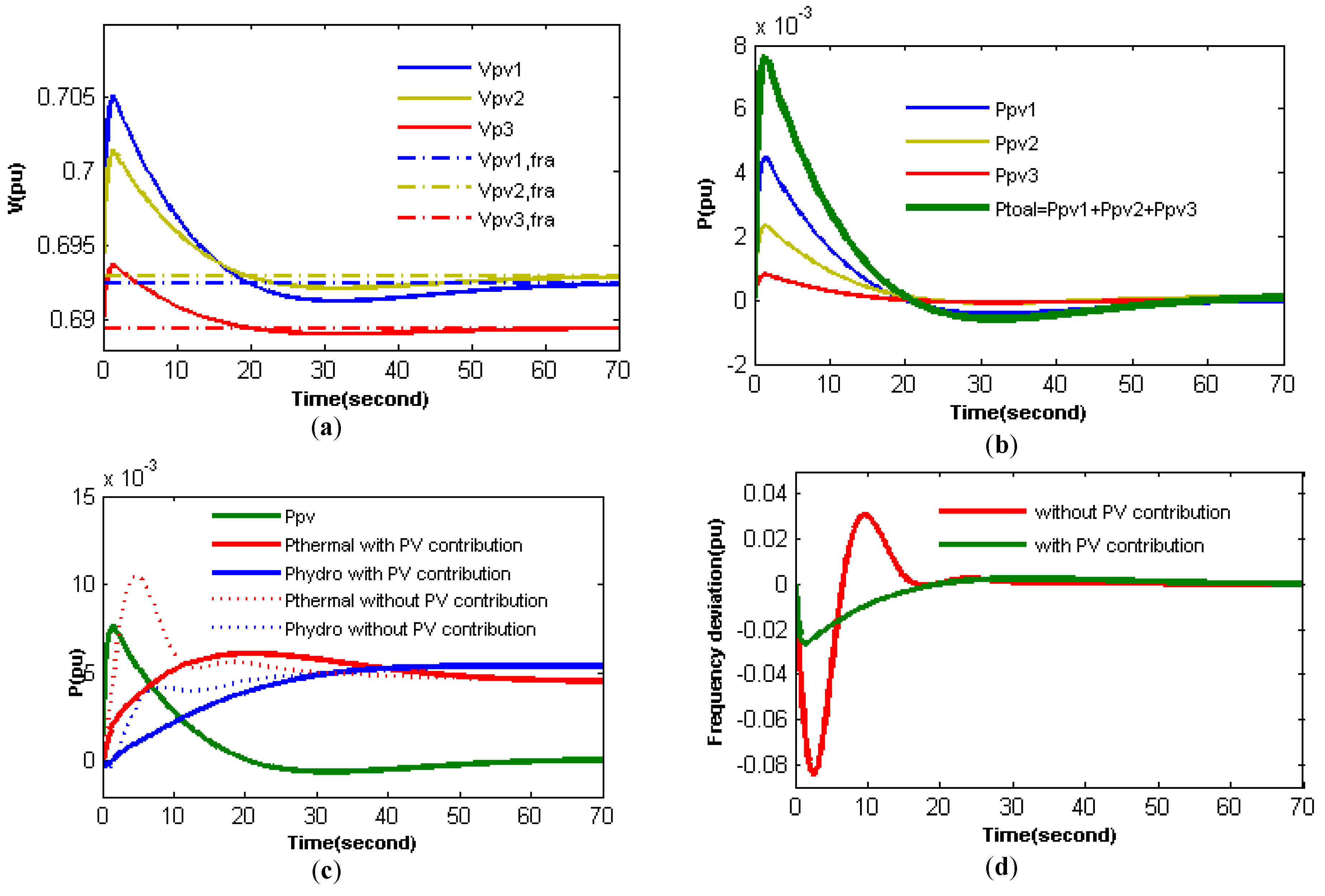
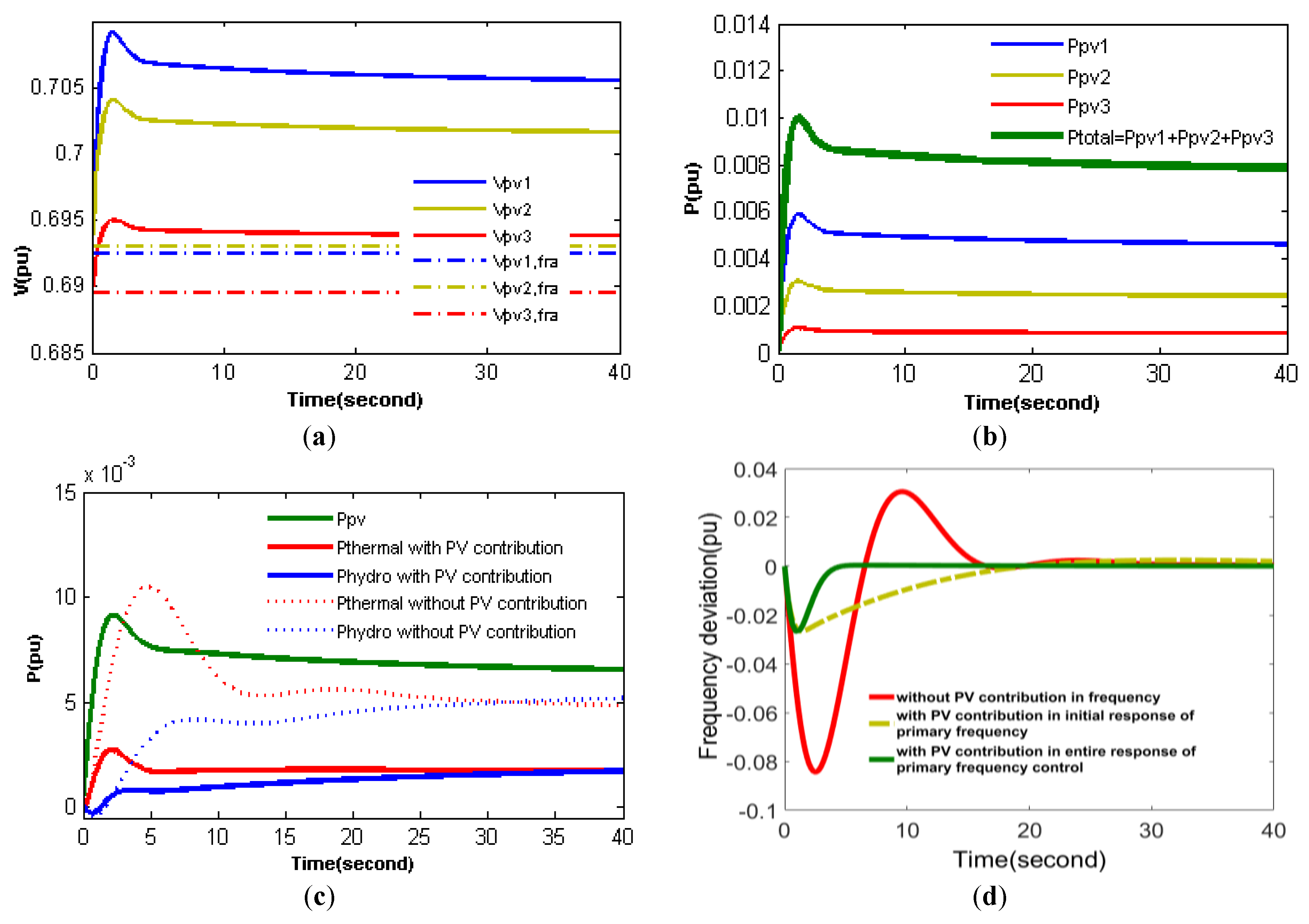
With the aim of PV contribution to the initial response of primary frequency control, the value of the in the PI controller, as expressed by Equation (7), has to be zero and the controller should have . The simulation results are shown in Figure 8 by applying the step load increase. The PVs’ voltage variation can be observed in Figure 8a. From the aforementioned figure it can be deduced that the PV voltage increases in line with Equation (7) and then returns to its previous state. Such changes result in the variation of the PV-produced power, as shown in Figure 8b.
Figure 8c presents the variation of PV (Ppv1 + Ppv2 + Ppv3), thermal, and hydro stations. It is clear that the variation in the power of hydro and thermal units diminished remarkably due to the contribution of the PV in the control of frequency, which results in a lower amount stress on such units. Furthermore, as shown in Figure 8c, PVs can respond quicker compared to thermal and hydro units.
Including PV generation in the frequency control considerably corrects the system frequency as can be observed in Figure 8d. By utilizing the newly amended objective for the optimal specification of the PI controller’s parameters, mitigation of the frequency overshoot was achieved.
4.3. PV System Involvement throughout Entire Primary Frequency Control
Due to the PV contribution in the entire range of primary frequency control, the PV systems’ PI controller has both and. The outcomes of this simulation can be observed in Figure 9. The PVs’ variation can be witnessed and further verified in Figure 9a. By analyzing the aforementioned Figure 9a, the voltage of the PVs rises as stipulated by Equation (7), and subsequently reaches a ceiling at a voltage higher than of the PVs since it includes PV systems over the entire range of control. Following the changes in the unit’s voltage, the PVs’ power varies as Figure 9b demonstrates. In addition, the power variation of PV (Ppv1 + Ppv2 + Ppv3), hydro, and thermal units is shown in Figure 9c. The variation in the power of the hydro and thermal units remarkably declined due to the PV effect in frequency control. Figure 9c indicates the faster response of the PV systems rather than the hydro and thermal units, a factor which helps the regulation of frequency. Additionally, Figure 9d displays system frequency. The frequency overshoot is correctly eliminated by utilizing an altered objective function. Overall, the participation of PV systems in initial primary control prevents a large frequency drop, whereas, by taking part in the entire primary control, PV systems allow a quicker recovering of frequency.
5. Development to a Two-Area Power System
In order to further gauge the performance of the suggested method, a two-area power system was considered for the next stage of simulations. The two areas are connected by a tie line. Each area consists of hydro, thermal, gas, and PV generation units. The transfer function of the proposed system with PV participation and contribution to frequency control is shown in Figure 10.
In this model, it is assumed that the PV unit in each area comprises two identical PV systems that experience 1000 w/m2 and 780 w/m2 irradiation in power system area 1 and 670 w/m2 and 420 w/m2 irradiation in power system area 2. are thermal, hydro, gas, and PV unit factors, respectively, and are considered to be 40%, 25%, 20%, and 15%.
In this case, the proposed controller (PID) is utilized, aimed at secondary frequency control, and its specifications were optimized by the PSO algorithm. In the two-area power system, the suggested objective function is as follows (10):
5.1. The Contribution of PV System in the Initial Response of Primary Frequency Control
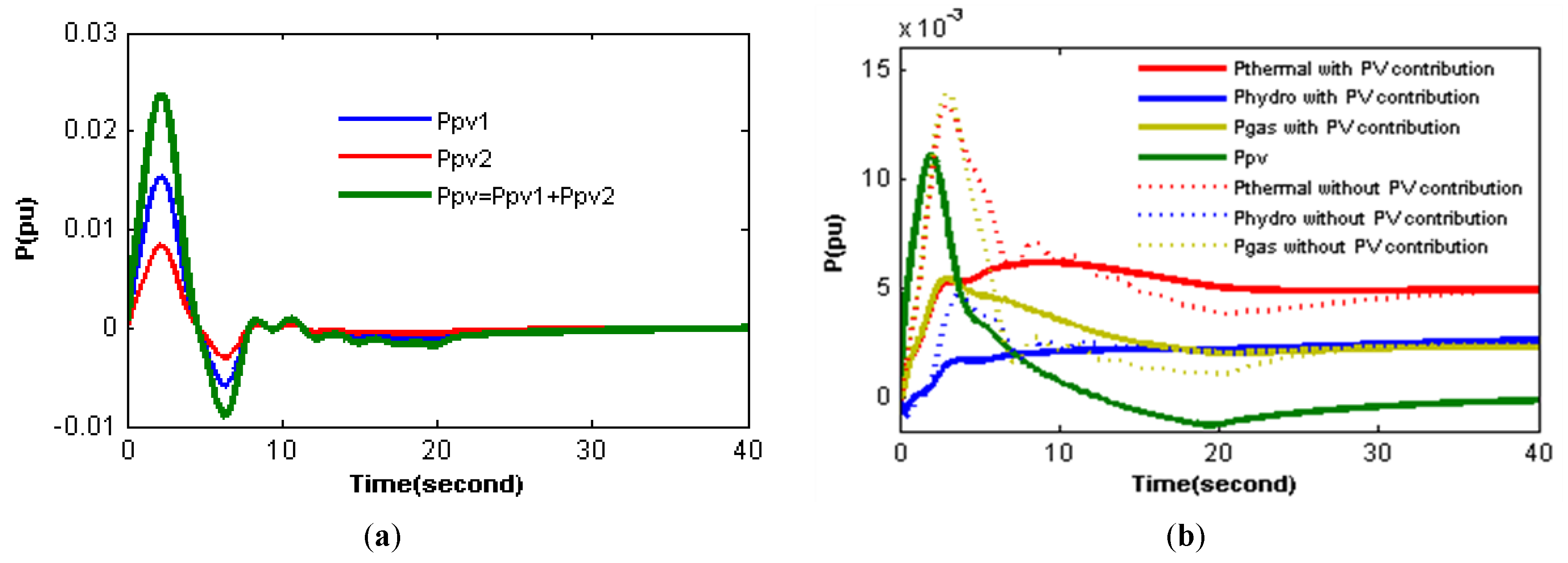
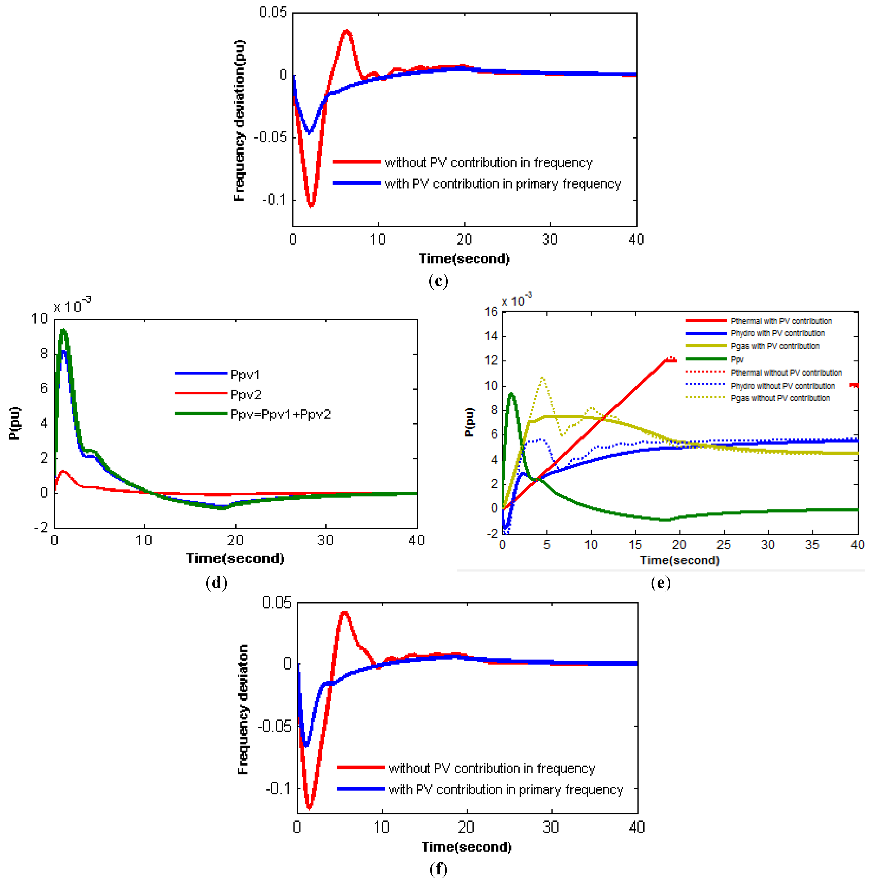
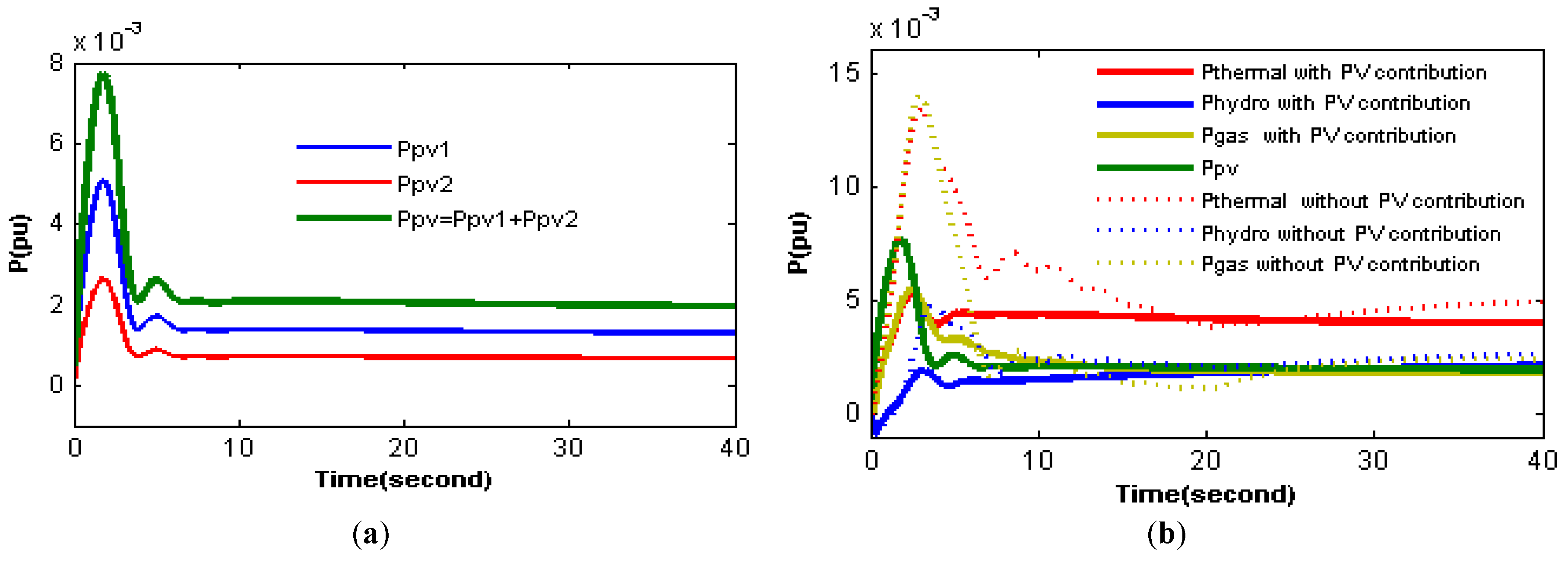
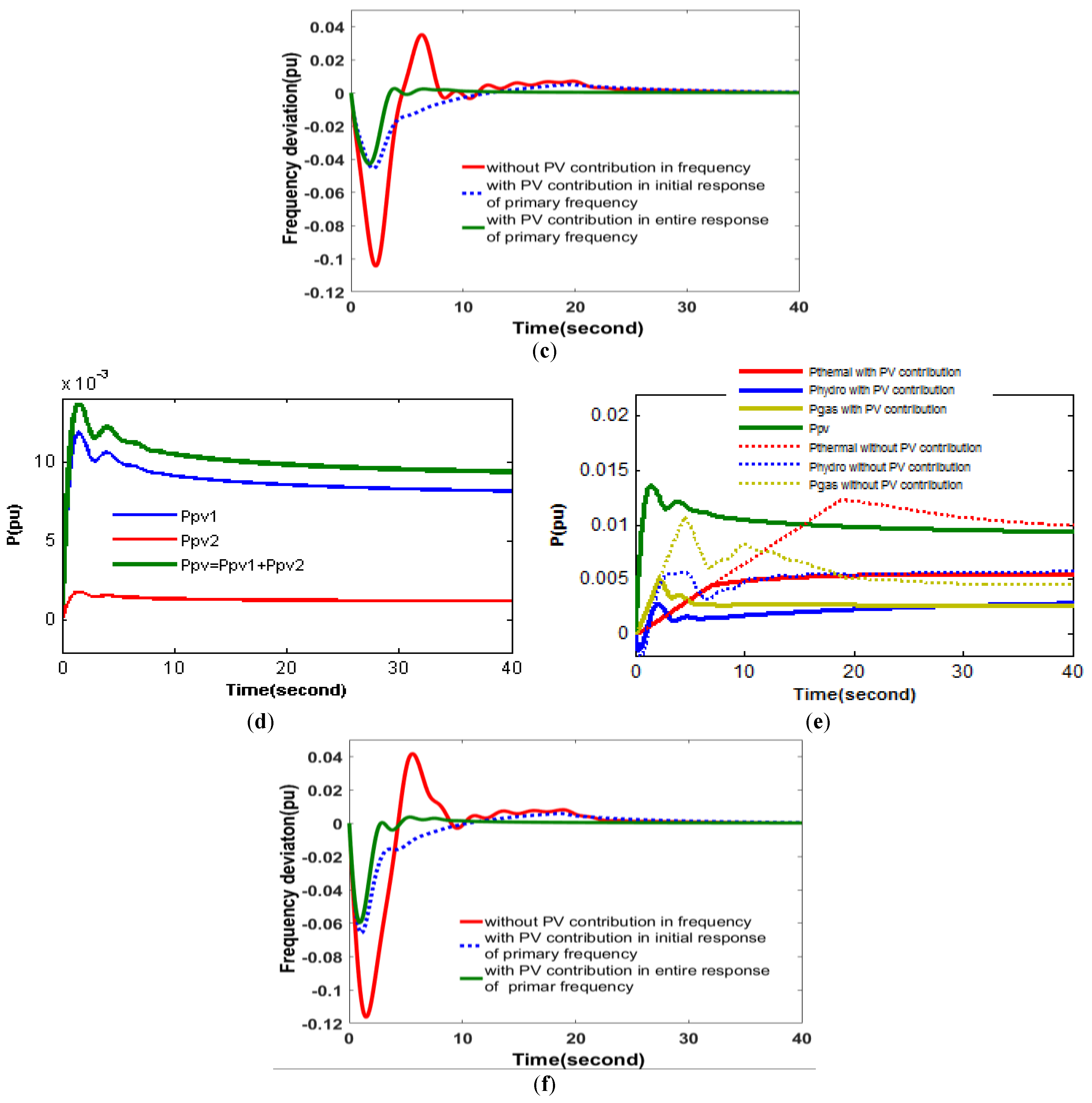
To only involve the PV systems in the initial part of the primary frequency control, the value of in the proposed PI controllers, as stipulated in Equation (7), is set to zero, and the controllers only have the proportional component (). The corresponding simulation outcomes are depicted in Figure 11. The PV powers change as shown in Figure 11a,d. In addition, Figure 11b,e shows the variation of the generation of thermal, hydro, gas, and PV (Ppv1 + Ppv2) units in areas 1 and 2. As can be seen, PV systems respond quickly when compared to hydro, gas, and thermal units. Therefore, the involvement of a PV system in the control of the frequency with an altered objective function improves the system frequency significantly (decreases undershoot, overshoot, and settling time) as depicted in Figure 11c for area 1 and Figure 11f for area 2. Furthermore, the variation in the power of the hydro and thermal units due to a frequency event is remarkably decreased, which means placing a lower amount of stress on such types of units.
5.2. The Contribution of the PV System throughout Entire Primary Frequency Control
For contribution of the PV systems across the entire primary frequency control, the suggested PI controllers, as stipulated in Equation (7), are required to have both proportional and integral components “ and ”. The simulation results pertaining to this case are shown in Figure 12. The power of PVs varies as given in Figure 12a for area 1 and Figure 12d for area 2. Furthermore, the variation of PV (Ppv1 + Ppv2), hydro, thermal, and gas units are illustrated in Figure 12b,e. Evidently, the variation in the power of the hydro, thermal, and gas units is diminished significantly by PVs’ contribution to frequency control, meaning less stress for these units. Figure 12b,e shows that the PV system’s response is much faster than thermal, hydro, and gas units. Hence, including the PV system in frequency control with a modified objective function based on the controller parameters’ optimization, considerably improves the system’s frequency (the undershoot, overshoot, and settling time decrease) as depicted in Figure 12c for area 1 and Figure 12f for area 2. The PV systems’ primary control avoids excessively steep frequency decreases and the PV systems’ secondary control assists the frequency to recover rapidly and efficiently.
6. Conclusions
A new type of model for power reservation in PV systems was proposed in this study by making PV systems contribute to the frequency control. The parameters of the PI controller for the PV system are achieved by the PSO algorithm through an adapted objective function. In order to study the operation and performance of the proposed system, a step load rise was used. The results show that the response of the system visibly improved due to the PVs’ contribution to the control of frequency. More precisely, the amount of overshoot almost reached zero in both one-area and two-area systems. In addition, the amount of undershoot has fallen by up to 60% (from 0.104 to 0.042) and 50% (from 0.118 to 0.06) in one-area and two-area systems, respectively. Regarding settling time, it is clear that it had a negligible enhancement in the one-area system, but it indicated a significant boost in the two-area system, in which it declined from about 25 s to 6 s with the help of the proposed technique. In conclusion, in an island microgrid, the stability of the overall system is improved with the proposed method and the need for ES devices is eliminated to a certain extent. The benefits are that in larger grids, it lowers the cost associated with capital investment in the system, and lower fuel consumption is required for the spinning reserve, thus mitigating the stress imposed on the available power plants. Future studies may consider high penetration of PV systems in power grids and investigate the possibility of applying the proposed approach to that situation. In addition, it would be useful to study PV contribution in ancillary services when there are other types of renewable energy, such as wind power, in the grid.
Author Contributions
All authors worked on this manuscript together and all authors have read and approved the final manuscript.
Funding
This research received no external funding.
Conflicts of Interest
The authors declare no conflict of interest.
Nomenclature
| ACE | area control error |
| Prt | rated capacity of the area, MW |
| f | nominal system frequency, Hz |
| D | system damping of area, pu MW/Hz |
| TSG | speed governor time constant, s |
| TT | steam turbine time constant, s |
| TPS | power system time constant, s |
| RTH | governor speed regulation parameters of thermal unit |
| RHY | governor speed regulation parameters of hydro unit Hz/pu MW |
| RG | governor speed regulation parameters of gas unit, Hz/pu MW |
| KPS | power system gain, Hz/pu MW |
| KR | steam turbine reheat constant |
| TR | steam turbine reheat time constant, s |
| TW | nominal starting time of water in penstock, s |
| TRS | hydro turbine speed governor reset time, s |
| TRH | hydro turbine speed governor transient droop time constant, s |
| TGH | hydro turbine speed governor main servo time constant, s |
| XG | lead time constant of gas turbine speed governor, s |
| YG | lag time constant of gas turbine speed governor, s |
| cg | gas turbine valve positioner |
| bg | gas turbine constant of valve positioner, s |
| TF | gas turbine fuel time constant, s |
| TCR | gas turbine combustion reaction time delay, s |
| TCD | gas turbine compressor discharge volume-time constant, s |
| n | the number of modules in the PV system |
| the maximum power of each module | |
| fractional power of each module | |
| reserve power of each module | |
| total reserve for all modules |
Appendix A
| s | |
References
- Saeed Uz Zaman, M.; Bukhari, S.B.A.; Hazazi, K.M.; Haider, Z.M.; Haider, R.; Kim, C.H. Frequency response analysis of a single-area power system with a modified lfc model considering demand response and virtual inertia. Energies 2018, 11, 787. [Google Scholar] [CrossRef]
- Rahman, M.M.; Chowdhury, A.H.; Hossain, M.A. Improved load frequency control using a fast acting active disturbance rejection controller. Energies 2017, 10, 1718. [Google Scholar] [CrossRef]
- Tavakoli, M.; Pouresmaeil, E.; Adabi, J.; Godina, R.; Catalão, J.P.S. Load-frequency control in a multi-source power system connected to wind farms through multi terminal HVDC systems. Comput. Oper. Res. 2018, 96, 305–315. [Google Scholar] [CrossRef]
- Bevrani, H.; Ghosh, A.; Ledwich, G. Renewable energy sources and frequency regulation: Survey and new perspectives. IET Renew. Power Gener. 2010, 4, 438–457. [Google Scholar] [CrossRef]
- Acharya, S.; Moursi, M.S.E.; Al-Hinai, A. Coordinated frequency control strategy for an islanded microgrid with demand side management capability. IEEE Trans. Energy Convers. 2018, 33, 639–651. [Google Scholar] [CrossRef]
- Balamurugan, M.; Sahoo, S.K.; Sukchai, S. Application of soft computing methods for grid connected PV system: A technological and status review. Renew. Sustain. Energy Rev. 2017, 75, 1493–1508. [Google Scholar] [CrossRef]
- Salam, Z.; Ahmed, J.; Merugu, B.S. The application of soft computing methods for MPPT of PV system: A technological and status review. Appl. Energy 2013, 107, 135–148. [Google Scholar] [CrossRef]
- Mahmood, H.; Michaelson, D.; Jiang, J. A Power Management Strategy for PV/Battery Hybrid Systems in Islanded Microgrids. IEEE J. Emerg. Sel. Top. Power Electron. 2014, 2, 870–882. [Google Scholar] [CrossRef]
- Mahmood, H.; Michaelson, D.; Jiang, J. Strategies for independent deployment and autonomous control of pv and battery units in islanded microgrids. IEEE J. Emerg. Sel. Top. Power Electron. 2015, 3, 742–755. [Google Scholar] [CrossRef]
- Marinic-Kragic, I.; Nizetic, S.; Grubisic-Cabo, F.; Papadopoulos, A. Analysis of flow separation effect in the case of the free-standinf photovoltaic panel exposed to various operating conditions. J. Clean. Prod. 2018, 174, 53–64. [Google Scholar] [CrossRef]
- Hoke, A.F.; Shirazi, M.; Chakraborty, S.; Muljadi, E.; Maksimovic, D. Rapid active power control of photovoltaic systems for grid frequency support. IEEE J. Emerg. Sel. Top. Power Electron. 2017, 5, 1154–1163. [Google Scholar] [CrossRef]
- Sekhar, P.C.; Mishra, S. Storage free smart energy management for frequency control in a diesel-PV-fuel cell-based hybrid AC microgrid. IEEE Trans. Neural Netw. Learn. Syst. 2016, 27, 1657–1671. [Google Scholar] [CrossRef] [PubMed]
- Mahmood, H.; Michaelson, D.; Jiang, J. Decentralized power management of a PV/battery hybrid unit in a droop-controlled islanded microgrid. IEEE Trans. Power Electron. 2015, 30, 7215–7229. [Google Scholar] [CrossRef]
- Kewat, S.; Singh, B.; Hussain, I. Power management in PV-battery-hydro based standalone microgrid. IET Renew. Power Gener. 2018, 12, 391–398. [Google Scholar] [CrossRef]
- Shuvra, M.A.; Chowdhury, B.H. Frequency regulation using smart inverters in high penetration distributed PV scenario. In Proceedings of the 2018 9th IEEE International Symposium on Power Electronics for Distributed Generation Systems (PEDG), Charlotte, NC, USA, 25–28 June 2018; pp. 1–5. [Google Scholar] [CrossRef]
- Jafarian, H.; Cox, R.; Enslin, J.H.; Bhowmik, S.; Parkhideh, B. Decentralized active and reactive power control for an AC-stacked PV inverter with single member phase compensation. IEEE Trans. Ind. Appl. 2018, 54, 345–355. [Google Scholar] [CrossRef]
- Liao, S.; Xu, J.; Sun, Y.; Bao, Y.; Tang, B. Wide-area measurement system-based online calculation method of PV systems de-loaded margin for frequency regulation in isolated power systems 2018. IET Renew. Power Gener. 2018, 12, 335–341. [Google Scholar] [CrossRef]
- Hoke, A.; Maksimović, D. Active power control of photovoltaic power systems. In Proceedings of the 2013 1st IEEE Conference on Technologies for Sustainability (SusTech), Portland, OR, USA, 1–2 August 2013; pp. 70–77. [Google Scholar]
- Datta, M.; Senjyu, T.; Yona, A.; Funabashi, T.; Kim, C. A Frequency-control approach by photovoltaic generator in a PV–diesel hybrid power system. IEEE Trans. Energy Convers. 2011, 26, 559–571. [Google Scholar] [CrossRef]
- Datta, M.; Senjyu, T.; Yona, A.; Funabashi, T. Minimal-order observer-based coordinated control method for isolated power utility connected multiple photovoltaic systems to reduce frequency deviations. IET Renew. Power Gener. 2010, 4, 153–164. [Google Scholar] [CrossRef]
- Liu, Y.; Xin, H.; Wang, Z.; Gan, D. Control of virtual power plant in microgrids: A coordinated approach based on photovoltaic systems and controllable loads. IET Gener. Transm. Distrib. 2015, 9, 921–928. [Google Scholar] [CrossRef]
- Pappu, V.A.K.; Chowdhury, B.; Bhatt, R. Implementing frequency regulation capability in a solar photovoltaic power plant. In Proceedings of the North American Power Symposium 2010, Arlington, TX, USA, 26–28 September 2010; pp. 1–6. [Google Scholar]
- Kumar, P.; Kothari, D.P. Recent philosophies of automatic generation control strategies in power systems. IEEE Trans. Power Syst. 2005, 20, 346–357. [Google Scholar] [CrossRef]
- Murty, P.S.R. Chapter 18—Power System Stability. In Electrical Power Systems; Murty, P.S.R., Ed.; Butterworth-Heinemann: Boston, MA, USA, 2017; pp. 479–526. ISBN 978-0-08-101124-9. [Google Scholar]
- Elgerd, O.I.; Fosha, C.E. Optimum megawatt-frequency control of multiarea electric energy systems. IEEE Trans. Power Appar. Syst. 1970, PAS-89, 556–563. [Google Scholar] [CrossRef]
- Parmar, K.P.S.; Majhi, S.; Kothari, D.P. Load frequency control of a realistic power system with multi-source power generation. Int. J. Electr. Power Energy Syst. 2012, 42, 426–433. [Google Scholar] [CrossRef]
- Ela, E.; Milligan, M.; Kirby, B. Operating Reserves and Variable Generation; Contract No. DE-AC36-08GO28308; National Renewable Energy Laboratory (NREL): Golden, CO, USA, 2011. [Google Scholar]
- Pouresmaeil, E.; Mehrasa, M.; Godina, R.; Vechiu, I.; Rodríguez, R.L.; Catalão, J.P.S. Double synchronous controller for integration of large-scale renewable energy sources into a low-inertia power grid. In Proceedings of the 2017 IEEE PES Innovative Smart Grid Technologies Conference Europe (ISGT-Europe), Torino, Italy, 26–29 September 2017; pp. 1–6. [Google Scholar]
- Rebours, Y.G.; Kirschen, D.S.; Trotignon, M.; Rossignol, S. A survey of frequency and voltage control ancillary services—Part I: Technical features. IEEE Trans. Power Syst. 2007, 22, 350–357. [Google Scholar] [CrossRef]
- Brissette, A.; Hoke, A.; Maksimović, D.; Pratt, A. A microgrid modeling and simulation platform for system evaluation on a range of time scales. In Proceedings of the 2011 IEEE Energy Conversion Congress and Exposition, Phoenix, AZ, USA, 17–22 September 2011; pp. 968–976. [Google Scholar]
- Chandorkar, M.C.; Divan, D.M.; Adapa, R. Control of parallel connected inverters in standalone AC supply systems. IEEE Trans. Ind. Appl. 1993, 29, 136–143. [Google Scholar] [CrossRef] [Green Version]
- Crossland, A.F.; Jones, D.; Wade, N.S.; Walker, S.L. Comparison of the location and rating of energy storage for renewables integration in residential low voltage networks with overvoltage constraints. Energies 2018, 11, 2041. [Google Scholar] [CrossRef]
- Yan, X.; Li, J.; Wang, L.; Zhao, S.; Li, T.; Lv, Z.; Wu, M. Adaptive-MPPT-based control of improved photovoltaic virtual synchronous generators. Energies 2018, 11, 1834. [Google Scholar] [CrossRef]
- Akbari, H.; Browne, M.C.; Ortega, A.; Huang, M.J.; Hewitt, N.J.; Norton, B.; McCormack, S.J. Efficient energy storage technologies for photovoltaic systems. Sol. Energy 2018. [Google Scholar] [CrossRef]
- Tavakoli, M.; Shokridehaki, F.; Funsho Akorede, M.; Marzband, M.; Vechiu, I.; Pouresmaeil, E. CVaR-based energy management scheme for optimal resilience and operational cost in commercial building microgrids. Int. J. Electr. Power Energy Syst. 2018, 100, 1–9. [Google Scholar] [CrossRef]
- Rodrigues, E.M.G.; Godina, R.; Catalão, J.P.S. Modelling electrochemical energy storage devices in insular power network applications supported on real data. Appl. Energy 2017, 188, 315–329. [Google Scholar] [CrossRef]
- Casey, L.F.; Schauder, C.; Cleary, J.; Ropp, M. Advanced inverters facilitate high penetration of renewable generation on medium voltage feeders-impact and benefits for the utility. In Proceedings of the 2010 IEEE Conference on Innovative Technologies for an Efficient and Reliable Electricity Supply, Waltham, MA, USA, 27–29 September 2010; pp. 86–93. [Google Scholar]
- Hoke, A.; Butler, R.; Hambrick, J.; Kroposki, B. Steady-state analysis of maximum photovoltaic penetration levels on typical distribution feeders. IEEE Trans. Sustain. Energy 2013, 4, 350–357. [Google Scholar] [CrossRef]
- Zabihi, S.; Zare, F. A new adaptive hysteresis current control with unipolar PWM used in active power filters. Aust. J. Electr. Electron. Eng. 2008, 4, 9–16. [Google Scholar] [CrossRef]
- Zabihi, S.; Zare, F. Active power filters with unipolar pulse width modulation to reduce switching losses. In Proceedings of the 2006 International Conference on Power System Technology, Chongqing, China, 22–26 October 2006; pp. 1–5. [Google Scholar]
- Zare, F.; Zabihi, S.; Ledwich, G. An adaptive hysteresis current control for a multilevel inverter used in an active power filter. In Proceedings of the 2007 European Conference on Power Electronics and Applications, Aalborg, Denmark, 2–5 September 2007; pp. 1–8. [Google Scholar]
- Zabihi, S.; Zare, F. An adaptive hysteresis current control based on unipolar pwm for active power filters. In Proceedings of the 2006 Australasian Universities Power Engineering Conference, Melbourne, Australia, 10–13 December 2006. [Google Scholar]
- Ishaque, K.; Salam, Z.; Shamsudin, A.; Amjad, M. A direct control based maximum power point tracking method for photovoltaic system under partial shading conditions using particle swarm optimization algorithm. Appl. Energy 2012, 99, 414–422. [Google Scholar] [CrossRef]
- Eberhart, R.C.; Shi, Y.; Kennedy, J. Swarm Intelligence, 1st ed.; Morgan Kaufmann: San Francisco, CA, USA, 2001; ISBN 978-1-55860-595-4. [Google Scholar]
- Zhu, M.; Li, J.; Chang, D.; Zhang, G.; Chen, J. Optimization of antenna array deployment for partial discharge localization in substations by hybrid particle swarm optimization and genetic algorithm method. Energies 2018, 11, 1813. [Google Scholar] [CrossRef]
- Seyedmahmoudian, M.; Jamei, E.; Thirunavukkarasu, G.S.; Soon, T.K.; Mortimer, M.; Horan, B.; Stojcevski, A.; Mekhilef, S. Short-term forecasting of the output power of a building-integrated photovoltaic system using a metaheuristic approach. Energies 2018, 11, 1260. [Google Scholar] [CrossRef]
Figure 1.
Schematic of the system under study.

Figure 2.
A linear block diagram of the suggested scheme.

Figure 3.
Updating the position of a particle vector.

Figure 4.
The Power-Voltage curve of a typical module (BP MSX 60).

Figure 5.
Irradiation received by module.

Figure 6.
Module power.

Figure 7.
A linear block diagram of the photovoltaic (PV)system contributing to the frequency control.
Figure 7.
A linear block diagram of the photovoltaic (PV)system contributing to the frequency control.

Figure 8.
The response of the system in reply to a 1% rise in step load in the initial response of primary frequency control: (a) Voltage variation of the PV modules; (b) Power variation of the PV modules; (c) Power variation in different units; (d) Frequency of the System.
Figure 8.
The response of the system in reply to a 1% rise in step load in the initial response of primary frequency control: (a) Voltage variation of the PV modules; (b) Power variation of the PV modules; (c) Power variation in different units; (d) Frequency of the System.

Figure 9.
The response of the system in reply to a 1% rise in step load throughout the entire primary frequency control: (a) Voltage variation of the PV modules; (b) Power variation of the PV modules; (c) Power variation in different units; (d) Frequency of the System.
Figure 9.
The response of the system in reply to a 1% rise in step load throughout the entire primary frequency control: (a) Voltage variation of the PV modules; (b) Power variation of the PV modules; (c) Power variation in different units; (d) Frequency of the System.

Figure 10.
Linear model of the two-area power system.

Figure 11.
The system response to PV contribution in the initial part of primary frequency control with a 1% rise in step load in power system area 1 and a 2% rise in step load in power system area 2: (a) Power variation of the PV modules in area 1; (b) Power variation in different units in area 1; (c) Frequency of the system in area 1; (d) Power variation of the PV modules in area 2; (e) Power variation in different units in area 1; (f) Frequency of the system in area 2.


Figure 12.
System response to PV contribution in primary frequency control with a 1% rise in step load in power system area 1 and a 2% rise in step load in power system area 2: (a) Power variation of the PV modules in area 1; (b) Power variation in different units in area 1; (c) Frequency of the system in area 1; (d) Power variation of the PV modules in area 2; (e) Power variation in different units in area 1; (f) Frequency of the system in area 2.


Table 1.
Weighting factor corresponding to different irradiations.
| Irradiation (w/m2) | D |
|---|---|
| 400–500 | 1 |
| 500–600 | 2 |
| 600–700 | 3 |
| 700–800 | 4 |
| 800–900 | 5 |
| 900–1000 | 6 |
© 2018 by the authors. Licensee MDPI, Basel, Switzerland. This article is an open access article distributed under the terms and conditions of the Creative Commons Attribution (CC BY) license (http://creativecommons.org/licenses/by/4.0/).
Share and Cite
MDPI and ACS Style
Tavakkoli, M.; Adabi, J.; Zabihi, S.; Godina, R.; Pouresmaeil, E. Reserve Allocation of Photovoltaic Systems to Improve Frequency Stability in Hybrid Power Systems. Energies 2018, 11, 2583. https://doi.org/10.3390/en11102583
AMA Style
Tavakkoli M, Adabi J, Zabihi S, Godina R, Pouresmaeil E. Reserve Allocation of Photovoltaic Systems to Improve Frequency Stability in Hybrid Power Systems. Energies. 2018; 11(10):2583. https://doi.org/10.3390/en11102583
Chicago/Turabian StyleTavakkoli, Mehdi, Jafar Adabi, Sasan Zabihi, Radu Godina, and Edris Pouresmaeil. 2018. "Reserve Allocation of Photovoltaic Systems to Improve Frequency Stability in Hybrid Power Systems" Energies 11, no. 10: 2583. https://doi.org/10.3390/en11102583
Note that from the first issue of 2016, this journal uses article numbers instead of page numbers. See further details here.