Energy and Exergy Analysis of a Cruise Ship †
by
 , , , and
Francesco Baldi
1,* ,
,
Fredrik Ahlgren
2,
Tuong-Van Nguyen
3,4,
Marcus Thern
5 and
Karin Andersson
6 1
Industrial Process and Energy Systems Engineering (IPESE), École Polytechnique Fédérale de Lausanne, 1950 Sion, Switzerland
2
Kalmar Maritime Academy, Linnaeus University, 39231 Kalmar, Sweden
3
Laboratory of Environmental and Thermal Engineering, Polytechnic School-University of São Paulo, São Paulo 05508-030, Brazil
4
Section of Thermal Energy, Department of Mechanical Engineering, Technical University of Denmark, 2800 Kongens Lyngby, Denmark
5
Energy Sciences, Lund University, 22100 Lund, Sweden
6
Department of Mechanics and Maritime Sciences, Chalmers University of technology, 41296 Gothenburg, Sweden
*
Author to whom correspondence should be addressed.
†
This paper is an extended version of our paper published in Baldi, F.; Ahlgren, F.; Nguyen, T.-V.; Andersson, K. Energy and Exergy Analysis of a cruise ship. In Proceedings of the International Conference on Efficiency, Cost, Optimization, Simulation and Environmental Impact of Energy Systems, Pau, France, 29 June–3 July 2015.
Energies 2018, 11(10), 2508; https://doi.org/10.3390/en11102508
Submission received: 17 August 2018
/
Revised: 11 September 2018
/
Accepted: 17 September 2018
/
Published: 20 September 2018
(This article belongs to the Section A: Sustainable Energy)
Abstract
:In recent years, the International Maritime Organization agreed on aiming to reduce shipping’s greenhouse gas emissions by 50% with respect to 2009 levels. Meanwhile, cruise ship tourism is growing at a fast pace, making the challenge of achieving this goal even harder. The complexity of the energy system of these ships makes them of particular interest from an energy systems perspective. To illustrate this, we analyzed the energy and exergy flow rates of a cruise ship sailing in the Baltic Sea based on measurements from one year of the ship’s operations. The energy analysis allows identifying propulsion as the main energy user (46% of the total) followed by heat (27%) and electric power (27%) generation; the exergy analysis allowed instead identifying the main inefficiencies of the system: while exergy is primarily destroyed in all processes involving combustion (76% of the total), the other main causes of exergy destruction are the turbochargers, the heat recovery steam generators, the steam heaters, the preheater in the accommodation heating systems, the sea water coolers, and the electric generators; the main exergy losses take place in the exhaust gas of the engines not equipped with heat recovery devices. The application of clustering of the ship’s operations based on the concept of typical operational days suggests that the use of five typical days provides a good approximation of the yearly ship’s operations and can hence be used for the design and optimization of the energy systems of the ship.
1. Introduction
1.1. Background
As humanity faces the global threat of climate change, society needs to drastically reduce greenhouse gas (GHG) emissions to the atmosphere. The transport sector is a significant contributor to the global CO emissions [1] and, within this category, the maritime sector contributes to approximately 2.7% of the global anthropogenic CO emissions [2]. While this contribution appears relatively low, the maritime sector will face difficult challenges. The demand for global trade, that mostly travels by sea, is expected to grow in the future [2]. At the same time, ships are still almost entirely powered by fossil fuels. While shipping will face the fierce competition against aviation and road transport for renewable fuels [3], ship energy systems need to become more energy efficient during the transition [4]. More generally, making shipping sustainable is a challenge that will demand growing attention by the shipping industry [5]. Recently, the International Maritime Organization (IMO) has officially adopted an initial strategy aiming at reducing GHG emissions from shipping by 50%, compared to 2008 levels, by 2050, and to work towards phasing out them entirely by the end of the century [6].
In this context, the cruise industry is facing an even greater challenge as it is growing at a greater pace. Cruise ship passengers have increased from 17.8 million in 2009 to 25.8 million in 2017 [7], and this growth is expected to continue in the coming years [7]. Cruise travels, with an estimated average of 160 kg CO per passenger and per day [8], are among the most carbon intensive in the whole tourism industry. The contribution of the cruise industry to global CO emissions was estimated to 19.3 Mtons annually in 2010 [8].
Altogether, these conditions present a challenge to the shipping companies who attempt to reduce their fuel consumption, environmental impact, and operative costs. A wide range of fuel saving solutions for shipping are available and partially implemented in the existing fleet, both from the design and operational perspective [9]. In this context, it has been acknowledged that the world fleet is heterogeneous, and measures need to be evaluated on a ship-to-ship basis [10]. In this process, a deeper understanding of energy use on board the specific ship is vital. Therefore, it is essential to improve our current understanding of the energy generation, conversion and use on board the cruise ship. In these regards, we believe that mapping all the different energy flows on board would allow gaining knowledge, useful for the improvement of current ships as well as for designing less energy intensive ships in the future.
1.2. Previous Work
The analysis of energy systems can be performed according to two, main approaches: model-driven, and data-driven.
Given the relative difficulty in obtaining good-quality datasets for system operations, in shipping as in other sectors, model-driven approaches are very widespread in scientific literature. According to a model-driven energy analysis, the system of interest is studied by first deriving a simplified representation using computational models, of various degrees of detail and complexity, and then using it to analyze its energy flows in one or more operational conditions. Shi et al. [11], for instance, developed the model of a cargo/passenger ferry and analyzed its propulsion power demand and efficiency at various ship speeds, and for a reference profile based on empirical experience. Theotokoats and Tzelepis [12] presented a generic model and showed its application to a Handymax size product carrier. In their study, they included the influence of the added resistance and studied its impact on a larger number of variables of interest, including various propulsive efficiencies, turbocharger speed, and exhaust gas temperature. Martelli et al. [13] also applied a generic modeling approach for the estimation of energy efficiency under various operational conditions, focusing on the application to small crafts. Other authors proposed alternative modeling strategies: Jafarzadeh et al. [14] proposed an approach based on the theory of bond graphs, while Yan et al. [15] used models based on neural networks. While these approaches help in estimating the influence of various operational and design parameters on the efficiency of the vessel, they do not provide information on how the vessel can be expected to be operated in real operational conditions, and rely on a series of assumptions that limit their ability to reproduce the behavior of a real vessel.
Data-driven approaches rely on actual measurements of relevant operational variables (such as ship speed, wind speed, engine power, engine fuel consumption) to analyze the performance of the vessel during a certain period of time. Data-driven models can thereby be used to provide suggestions on how to improve the system from an energy perspective. While this approach involves a loss of generality, as the reported results only represent the vessel used for data collection, they provide a more accurate picture of both the operational conditions and of the performance of the system. Yuan et al. [16] applied this approach to a small passenger vessel operated in the Yangtze river, analyzing the effect of environmental conditions. Galli et al. [17] analyzed performance parameters, such as trim, propulsion power demand and engine fuel consumption, for a full year of operations.
The largest set of published work in this field relates to the application to fishing vessels [18,19,20,21,22], where there is a high availability of studies applying the concept of energy audit to ship energy demand. Compared to other similar studies, these have the advantage of a presenting a more structured approach that subdivides the energy demands among different users on board and, hence, also takes auxiliary energy demand into account. This constitutes a major step forward compared to other literature in the field, that mostly focuses on propulsion power demand. However, these papers only focus on one specific field of application, and hence provide results that are only of relevance for the specific case of fishing vessels.
The main limitation of purely data-driven approaches is that they only provide information on what can be directly measured on board. While this provides a large amount of useful information, it is still limited to a handful of values, particularly in relation to energy efficiency. For this reason, some authors have proposed the use of a hybrid approach, where measured data are used as input values to a model of the system, thus allowing the calculation of performance indicators that cannot be directly measured on board. Coraddu et al. [23] used operational data for ship speed, displacement and sea state to estimate the value of the EEOI of a RO-PAX vessel based on real operational conditions; this brought them to challenge the assumption that a single EEOI can be calculated for a long period of operations. Simonsen et al. [24] used operational measurements from a cruise ship operated on the Norwegian coast to train a black-box model able to predict the total fuel consumption of the ship; they then used the model developed in the paper to test the validity of the application of the models suggested by the IMO to the evaluation of the energy efficiency of cruise ships. Baldi et al. [25] proposed the analysis of the performance and energy flows of a chemical tanker, based on one year of ship’s operations. For this purpose, they used simplified models of the ship energy systems to determine the flows and the performance indicators that could not be measured. There is in general, however, the need for larger set of case studies that can be used to test methods and technologies for ship energy efficiencies to relevant cases.
In addition to general considerations about the analysis of ship energy performance, there is a more specific limitation of existing literature in the lack of studies on the determination of the on-board heat demand. For most ship types, this is justified by the low demand and high availability from the waste heat of the engines. Baldi et al. [25], for instance, show that in the case of a product tanker the heat demand was estimated to account for roughly 20% of the total energy demand of the ship on a yearly basis. However, this only corresponds to 4.1% of the total fuel consumption (contribution of the auxiliary boilers), while the rest of the demand is fulfilled using waste heat.
Differently from other cases, the heat demand on cruise ships is significantly higher compared to standard cargo ships. Referring to winter conditions, Marty et al. [26] estimated the instantaneous heat demand of a selected cruise ship to reach roughly 23 MW, compared to an estimated peak of 49 MW for propulsion and electric auxiliaries combined . The work of Marty et al. [26], however, only focuses on one single trip, and little can be deduced on what the results would imply for the operation of the ship on the longer terms.
In recent years, several authors have studied the potential of improving the efficiency of a ship by recovering the waste heat from the Diesel engines (see Shu et al. [27] and Mondejar et al. [28] for a review of such applications), but mostly focused on maximizing the power output of the waste heat recovery (WHR) system. In the case of cruise ships, this might lead to an underestimation of the potential for system optimization. In the work of Mondejar et al. [29] concerning the optimization of an organic Rankine cycle (ORC) on a small cruise ship, the authors assumed that the existing facilities for fulfilling the heat demand on board are left as they are. Baldi et al. [30] attempted to optimize the load allocation among the different engines of the same case study, including considerations related to the efficiency of the heat generation on board. In their work, however, they did not consider the potential for optimizing the design of the system, nor did they take into account the temperature at which the heat has to be delivered to the different users.
1.3. Aim
Based on the limitations in scientific literature highlighted in the previous section, in this paper we aim at providing new insights on the energy system of a cruise ship. To do so, we propose an approach based on the use of energy and exergy analysis applied to the entirety of the energy system of the ship.
More specifically, with this work our aim is to:
- Analyze the demand of a cruise ship in terms of propulsion power, electric power and heat, based on operational measurements. The lack of existing information with reference to the heat demand is considered a particular element of novelty when compared to existing literature in the subject.
- Analyze the current efficiency of the system, and potential ways to improve it, by means of applying exergy analysis.
- Provide reference operational conditions and typical operational days for further use in the field of energy systems optimization.
2. Materials and Methods
In this paper, we present the application of energy and exergy analysis (described in Section 2.2) to a cruise ship. This is done for one specific case study vessel, described in Section 2.1, including the specifics of the available information, in particular the measured data and the technical documentation; the specific assumptions and methods used for processing the available information into energy and exergy flows are summarized in Section 2.3, while a more thorough description is provided in the Appendix A.
2.1. Case Study Vessel
The energy and exergy analysis are applied to a cruise ship operating daily cruises in the Baltic Sea between Stockholm and the island of Å land. The ship is 176.9 m long, has a beam of 28.6 m, and has a design speed of 21 knots. The ship was built in Aker Finnyards, Raumo Finland in 2004.
The ship has a capacity of 1800 passengers and has several restaurants, night clubs and bars, as well as saunas and pools. This means that the heat and electricity demands are expected to be higher compared to a cargo vessel of the same size. Typical ship’s operations, although they can vary slightly between different days, are represented in Figure 1. It should be noted that the ship stops and drifts in open sea during night hours before mooring at its destination in the morning, if allowed by weather conditions.
The ship systems are summarized in Figure 2, while a list of the main system components is provided in Table 1. The propulsion system is made of two propulsion lines, each composed of two engines, a gearbox, and a propeller. The main engines are four Wärtsilä 4-stroke Diesel engines (ME) rated 5850 kW each. All engines are equipped with selective catalytic reactors (SCR) for NO emissions abatement. Propulsion power is needed whenever the ship is sailing; however, it should be noted that the ship rarely sails at full speed, and most of the time it only needs one or two engines operated simultaneously.
Auxiliary power is provided by four auxiliary engines (AE) rated 2760 kW each. Auxiliary power is needed on board for several functions, such as summer refrigeration for the summer period (and, more generally, for the heating, ventilation, and air conditioning (HVAC) systems), bow thrusters, pumps in the engine room, lighting, and entertainment facilities for the passengers.
Auxiliary heat needs are fulfilled by the exhaust gas steam generators (HRSG), located on all four AEs and on two of the four MEs, by the heat recovery on the high-temperature (HT) cooling water systems (HRHT), and by the auxiliary, oil fired boilers (AB). The heat is needed for passenger and crew accommodation, as well as for the heating of the highly viscous heavy fuel oil used for engines and boilers. This last contribution, however, is drastically reduced since the 1st of January 2015. Starting from this date, new regulations entering into force require the use of low-sulfur fuels, which do not need to be heated at high temperature before injection. For the period investigated in this study, however, low-sulfur heavy fuel oil (LS-HFO) with a maximum sulfur content of 1% was used.
The operational data were collected on board from the ship’s machine logging and surveillance system for a one-year period, from the 3 December 2013 until the 2 December 2014. The data sampling rate was selected to 15 min, automatically calculated as averages over the respective periods by the on-board data logging systems. This sampling time was considered to be an acceptable compromise between accuracy and computational time required for the data processing. Data consistency was ensured by creating a descriptive statistic and a histogram for each measured variable. This allowed understanding the expected variation of the measured variables, and setting a filter for detecting and removing outliers. This was deemed necessary given the lack of more detailed information regarding the type, placement, and calibration status of each individual sensor.
Since measurements of ambient and seawater temperature from on-board logging systems were not available for the whole dataset, we used measurements from the Swedish Meteorological and Hydrological Institute (SMHI) [31]. We used data from the lighthouse “Landsort” for the seawater, and from the lighthouse Svenska Högarna for the ambient temperature, both located along the route of the vessel.
2.2. Energy and Exergy Analysis
2.2.1. Energy Analysis
Energy can be stored, transformed from one form to another (e.g., heat to power) and transferred between systems, but can neither be created nor destroyed (conservation law) [32]. The system under study is the ship energy system and is thus taken as control volume. The energy balance can be expressed as:
In Equation (2), the left-hand side represents, on a time rate basis, the energy associated with the fuel consumed in the boilers and engines () and the air used in the combustion processes (). The right-hand side denotes the power () and heat () required on-site (e.g., propulsion and fuel heating), and the heat discharged into the environment () with, for instance, the exhaust gases.
The energy flow associated with a material stream is calculated as the sum of the physical and chemical enthalpies, and kinetic and potential energies are neglected. The physical energy is taken as the relative enthalpy, as underlined in [33], and the chemical energy is taken as the lower/higher heating value. The environmental conditions taken for the present analysis are the ambient pressure (1.01 bar) and seawater temperature (measured).
2.2.2. Exergy Analysis
Exergy may be defined as the maximum theoretical useful work (shaft work or electrical work) as the system is brought into complete thermodynamic equilibrium with the thermodynamic environment while the system interacts with it only’ [34]. Unlike energy, exergy is not conserved but some is destroyed because of the irreversible phenomena taking place in real processes (e.g., chemical reactions such as combustion). The exergy balance for the system under study can be expressed as:
In Equation (4) the left-hand side represents, on a time rate basis, the exergy associated with the fuel and air. The right-hand side denotes the exergy of the waste streams, the exergy transfers with heat and power, and the exergy destroyed in the ship system. Kinetic and potential exergies are neglected, and the exergy of a given material stream is derived as the sum of the physical and chemical exergies. The chemical exergy is calculated based on the reference environment of [35], and its value is approximately equal to the higher heating value for hydrocarbon fuels. The exergy destruction can be calculated using the Gouy-Stodola theorem [33]. The exergy balance may alternatively be formulated as:
where is called the exergy product, and corresponds to the desired output of the system, in exergy terms (for example, the power produced in an engine). denotes the exergy fuel, and represents the resources spent to drive the studied process (for instance, the fuel used in a combustion process). The last term corresponds to the losses of a system, such as the heat discharged into the environment with cooling water.
2.2.3. System Performance
The following indicators are used to evaluate the system performance:
- the exergy efficiency , defined as the ratio between the exergy product and fuel of a given component or system:
- the efficiency defect , presented in the work of Kotas [33], defined as the fraction of the total exergy input destroyed in the successive irreversible processes:
- the irreversibility share , suggested in the work of Tsatsaronis [36], defined as the ratio between the exergy destroyed in the i-th component in relation to the exergy destroyed in the entire system:
2.3. Modeling the Energy System of the Ship
Not all of the variables that are required to perform a full energy and exergy analysis of the system are available from measurements. In some cases, they are measurable, but not measured (e.g., some temperatures, mass flows, etc.). In other cases, they are simply impossible, or impractical, to measure (e.g., specific enthalpy, specific entropy). For this reason, it was necessary to model the energy system of the ship, thereby allowing the calculation of the operational variables of interest that could not be directly measured.
The main principles applied to the modeling are presented in the following sections and summarized in Figure 3, while a more thorough description and validation of the different approaches is presented in Appendix A. The data were first processed by the main and AE modules to derive the related energy flows. These were then used to calculate the electric power demand, the energy flows in the cooling systems and, consequently, the heat recovered in the HTHR systems. This combined information was used to determine the heating demand. Finally, all calculated flows were aggregated to determine energy and exergy flows and related performance indicators.
2.3.1. Diesel Engines
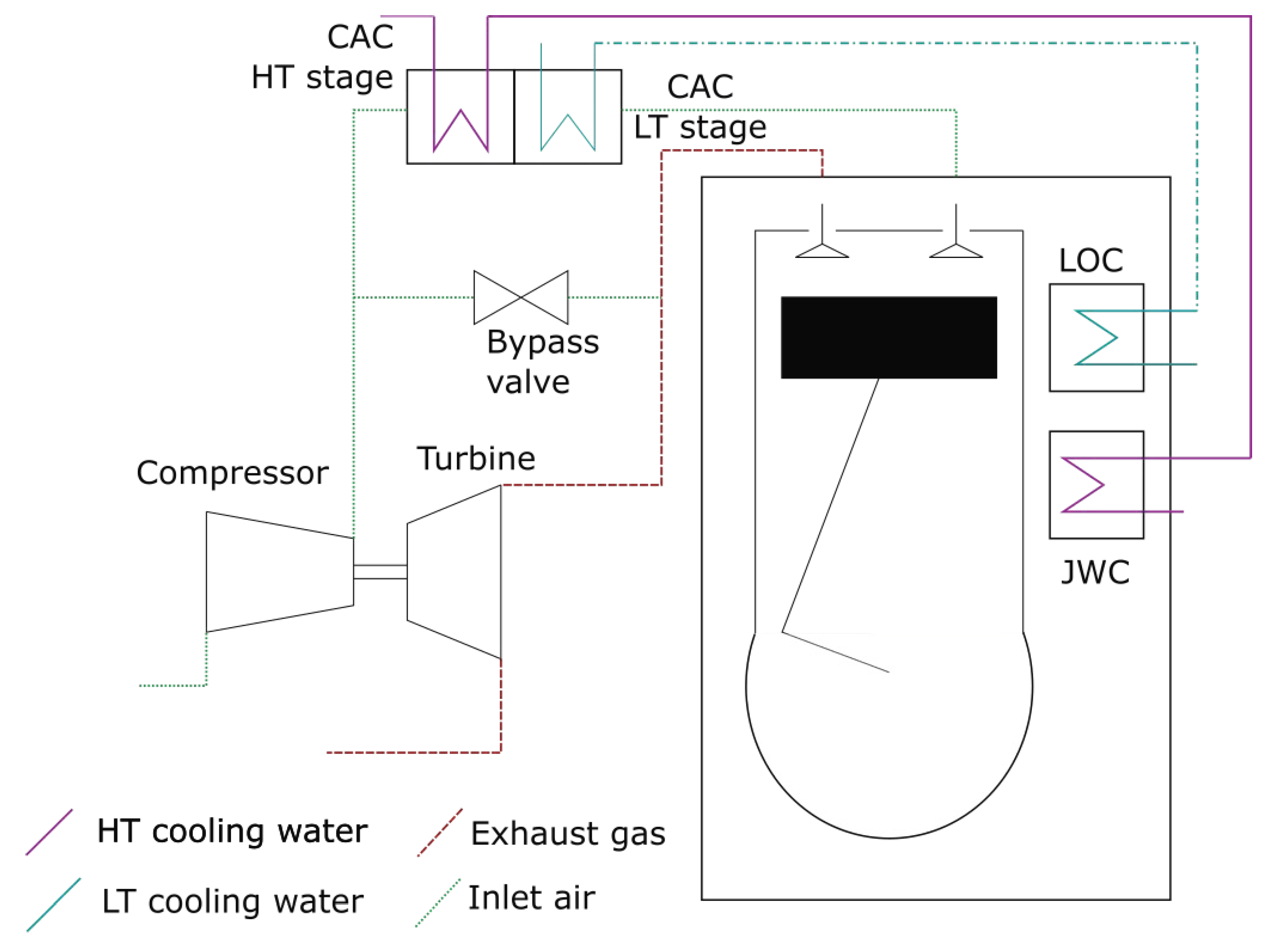
The Diesel engines are the only source of electric and mechanical power in the system, subdivided in four main engines for propulsion and four AEs for on-board electric power generation. The energy and exergy analysis of the engines is not limited to the boundary of the system, but is brought to the detail of the different components that constitute the engine systems, as shown in Figure 4.
The power output of the main engines was not measured and needed to be estimated. In this work, we calculated the engine power output based on measurements of engine fuel rack position (used as a proxy of the mass of fuel injected per cycle) and of the engine speed (see Equations (9)–()). In the case of the AEs, instead, direct measurements of the power generated by each engine were available.
In Equations (9)–(), , , , , and represent the fuel flow to the engine, the fuel rack position, the engine speed, the engine efficiency and the lower heating value of the fuel, respectively, and the subscript refers to design conditions.
For both auxiliary and main engines, parts of the relevant internal variables are not measured (particularly with relation to the bypass valves) and this required to determine them based on modeling the heat and mass balance of the engine. Values for temperatures, mass flows and energy flows for different engine loads are provided in Appendix A.2, for both main and AEs.
2.3.2. Electric Power Demand
The total electric power demand of the system () was estimated as the sum of the power generated by the four AEs (), that is directly measured on the electrical side of the generators and has a rather high accuracy.
The ship is equipped with a number of different systems, including lighting, navigational systems, pumps and compressors, etc. However, none of the individual contributions is directly measured. Hence, estimations of the energy demand of individual consumers needed to be based on indirect measurements. In this paper only the contributions of the HVAC and the bow thrusters were identified separately from the remaining parts of the system. More details about how these contributions were separated are provided in Appendix A.3.
2.3.3. Heating and Cooling Systems
The main view of the ship heating and cooling systems is presented in Figure 5. The case study ship is not provided with any means to directly measure the heat demand (e.g., steam flow meters) and cooling flows, and it was necessary to provide estimations based on other measurements and assumptions.
The ship’s cooling systems are designed similarly to most ships and divided in two cooling systems operated at two separate temperature levels: the HT cooling systems (70–90 C) and the low-temperature (LT) cooling systems (40–60 C). The cooling systems provide the necessary cooling to the engines, to the steam systems and to all other components on board.
All values not directly measured in the cooling systems were calculated based on mass and energy balances. Mass flows were determined based on measurements of the pressure in the system and on the performance curves of the cooling pumps as provided in the engine project guides.
The heat demand was subdivided among the contributions of the HVAC preheater () and reheater (), the hot water heater (), the HFO heaters () the tank heating systems for HFO () and other liquids (), the machinery space heating () and other tanks (). The heat generation is instead composed of the contribution of the exhaust gas boilers ( and ), the heat recovery from the HT cooling systems () and the boilers (). The heat demand and generation are summarized in Equations (13) and (14).
As a consequence of the limited amount of available data, we propose a method based on a combination of operational measurements and assumptions related to the behavior of the energy system for the determination of the heat demand and of its share among different consumers. According to this method, the demand and supply of heat on board are defined based on a number of unknown parameters, that are subsequently calculated using an optimization procedure with the aim of minimizing the error on the monthly fuel consumption from the boilers. This value was made available from operational data manually logged by the ship’s crew. A more detailed description of this procedure is provided in Appendix A.4.
2.4. Operational Mode
The ship operates in different conditions, and it can be useful to provide a separate analysis depending on the operational mode. The four operational modes identified for the selected case study are defined as follows:
- High-speed sailing Ship speed above 15 kn
- Low-speed sailing Ship speed between 4 and 15 kn
- Maneuvering Ship speed between 2 and 4 knots OR Thrusters power larger than 0
- Port stays/ship drifting All other points
The selection of the four operational modes was performed based on standard practices in the analysis of maritime operations, and on the specifics of the case study. The distinction between “Sailing”, “Maneuvering” and “Port stay” is typical for describing ship’s operations, and was hence taken as a starting point. Based on an exploratory analysis of the data, we could notice that the ship regularly stop at sea during night hours: this type of operation was merged with the “Port stays” operations, as they are equivalent from an energy analysis perspective. Finally, the low-speed and high-speed operational modes were separated, as the first refers to operational conditions according to a standard schedule, while the second refers to special operational conditions that occurred only a few times during the operational period analyzed in this study.
2.5. Determination of Typical Operational Conditions
Improving the performance of a ship requires a detailed analysis of the energy demands to optimize the dimensioning and operation of the technologies and processes to install on board. It requires the analysis of the hourly, daily and seasonal variations of the heat/power consumption, operating (e.g., ship speed) and external conditions (e.g., air temperature). However, gathering and processing those data may be time-consuming because of the high number of points to assess. It is therefore desirable to reduce this large quantity of information while keeping the relevant details on the relations between the variables of interest. This can be done by representing these yearly profiles in a limited number of (typical) periods, avoiding the repetition of similar data sets. Clustering consists of grouping such sets in a single group (cluster) so that the items in the same group are more like each other than to those belonging to other groups. Several algorithms are introduced in the literature to partition these datasets. The one selected in this work is the Lloyd’s (k-means) algorithm [37], which is a non-deterministic method computationally faster than conventional hierarchical tools. The approach originally proposed by Fazlollahi et al. [38] for energy systems was used to select the optimum number of clusters (). The general principle for the choice of () states that it should be as low as possible for data handling purposes, while preserving a high accuracy of the retrieved data. It builds on the calculation of three criteria:
- the average intra-cluster distance to assess the density of each cluster, preferably small;
- the average inter-cluster distance to assess the distance between each, preferably high;
- the expected square error, a statistical measure of the accuracy of the reconstructed profile, preferably low;
In parallel, the cluster quality was systematically evaluated by calculating the following performance indicators:
- the profile deviation (deviation between original and typical period profiles), ;
- the deviation from the load duration curve of the average values of each period, ;
- the relative error in load duration curve deviation ;
- the maximum duration load curve difference ;
- the number of periods with relative errors higher than 7%.
This set of performance objectives is defined as a set of constraints with an upper limit that should be respected when minimizing the number of clusters, applying the e-constraints algorithm. The dataset is further reduced by partitioning each typical day into a set of segments using a similar approach. The aim of the present clustering is to identify typical periods that are appropriate for improving the thermodynamic performance of ship energy systems. It can be achieved through either reducing the external energy demands (better energy management), e.g., with storage systems or internal recovery, or through implementing new technologies that result in higher fuel-to-demand efficiencies (better energy conversion). Hence, the attributes that are the primary focus of this study are:
- the total power consumption, including the mechanical and electrical loads;
- the total heating demand, further divided into the LT and HT needs, which is related to the external temperature;
- the total exergy destruction on-board, which quantifies the thermodynamic performance of the ship energy systems.
A one-year dataset with 35,040 time steps (sampling of 15 min) was selected and divided into typical periods based on these three attributes. The clustering approach proposed by Fazlollahi et al. [38] provides as output typical days having the same data frequency as the original time series (in this case, 15 min). From a computational perspective, however, this might not necessarily be the most efficient sampling. Operating conditions within a certain cluster (typical day) are often nearly constant for a longer time, suggesting that a variable time resolution would lead to a lower dimensionality of the data while retaining most of the original information. For this purpose, in this paper we employ the Adaptive Piecewise Constant Approximation (APCA) approach proposed by Keogh et al. [39].
3. Results
The results are divided in five main parts. In Section 3.1 an initial, exploratory analysis of the dataset is provided, including some descriptive analytic of variables of interest for the energy demand of the ship, such as engine loading and ambient conditions. In Section 3.2 and Section 3.3 the main results of the energy and exergy analysis are presented. The results of the clustering of the ship’s operations, with particular reference to the ship energy demand, into typical operational days is presented in Section 3.4.
3.1. Exploratory Analysis
Figure 6a,b represent the time evolution and the distribution over the year of the ambient air and sea water temperature. The relatively low temperatures that are experienced by the case study ship during its operations rise expectations for HVAC to be high in the heating part and low in the cooling part. On the other hand, the fact that, in summer, air temperatures reach up to 26 °C justify the existence of an HVAC unit that can also operate in cooling mode.
Figure 7 represents the distribution of the ship speed. The ship operates for almost the entire year according to a fixed schedule, while there are a couple of periods (particularly during the summer months) when the ship operates at higher speed. In Figure 8 it can be also observed that the ship spends a relatively large amount of time in port. These remarks suggest that, despite the high installed power of the main engines, the energy demand for propulsion is expected to be relatively low.
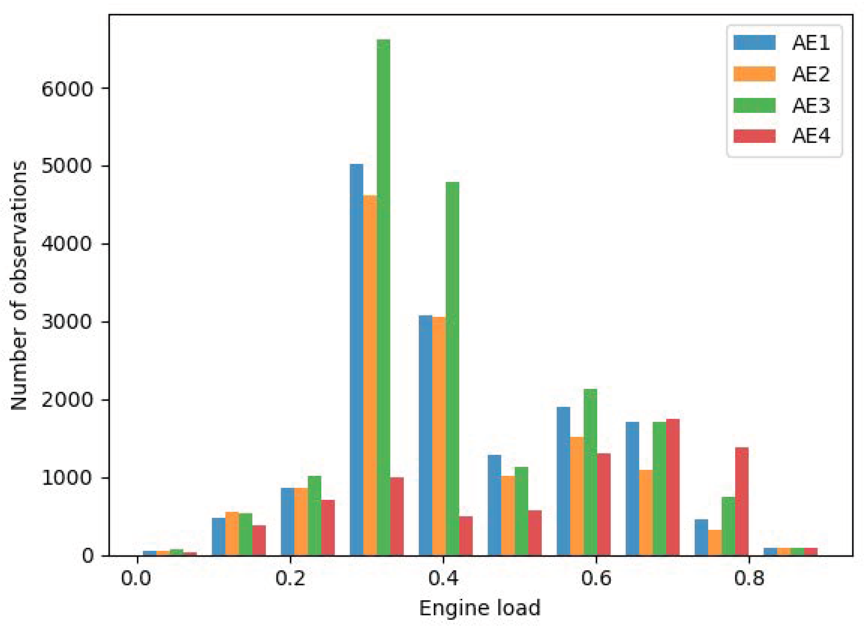
Figure 9 and Figure 10 show the frequency of the load at which each of the engines (main and auxiliary engines, respectively) are operated. The main engines are operated mostly at loads between 30% and 60%, despite the optimal load for the engines being located around 85%. This is a consequence of both the low speed at which the ship is generally operated, and of the fact that the two shaft lines are operated independently, and hence do not allow the use of only one of the four engines at high load.
A larger difference can be observed between the operations of the different AEs. AE-3 is generally more often operated, as it is the engine that is run in port with clean fuels. On the other hand, it seems that AE-4 is operated rarely, which might be due to maintenance issues during the selected period of analysis.
3.2. Energy Analysis
The ship’s energy demand is first subdivided among the different types of consumers. The evolution of the demands of propulsion, electric power, and heat over time during a typical voyage is shown in Figure 11 and Figure 12, representing a winter and a summer day respectively. As expected, the heating demand in winter is higher than in summer [2800–4500 kW vs. 1100–2900 kW], as a consequence of the reduced need for compartment heating. On the other hand, the electric power demand behaves inversely, ranging around 1900 kW during the reference winter day (peaks are connected to the use of thrusters in port for maneuvering) and around 2300 kW during the reference summer day, where the difference is mostly associated with the demand of the HVAC compressors. Looking at the yearly cumulated demand, nearly 50% of the total energy demand is related to ship propulsion (see Figure 13), while the remaining portion is approximately equally split between electric energy and heat demand.
The HVAC systems represents a minor contribution (3%) of the electric energy demand, as it is only used for a few months during summer. This is not surprising, since it can be observed that (see Figure 6b) the air temperature is always below 27 C, and rarely above 17 C. Also the thrusters, although their instantaneous power demand is high, are only used for a very short time each day and, hence, their total contribution to the ship electrical energy demand is limited to 1.5%.
Heat recovery has a large impact on the overall external heat demand (see Figure 14). The exhaust gas boilers and the heat recovery on the HT-water fulfill almost 75% of the yearly demand for heating, leaving only the remaining 25% to be provided by oil-fired auxiliary boilers, that eventually only represent a minor contribution to the total ship’s yearly fuel consumption (see Figure 15). The contribution of the HRSG and the HTHR is substantially constant throughout the year (Figure 16); the auxiliary boilers are used to cover the periods of mismatch between heat demand and availability of waste heat. These conditions generally happen during port stays (when there is no waste heat from the main engines) and during winter (when the heat demand is higher).
Looking on the heat demand, the HVAC preheater represents the largest contributor (56%) to the annual heating demand, followed by the hot water heater (18%) and by the galley (11%). In multi-season central HVAC systems the preheater is generally used for the main heating contribution during winter, while the reheater is only used for peak demand, or for adjusting the delivery air temperature during summer, thus explaining the large contribution of the former. The relatively large share of the hot water heater can instead be related to the fact that these systems are used during all seasons.
The full Sankey diagram representation of the energy flows on board is provided in Figure 17.
3.3. Exergy Analysis
The results of the exergy analysis of the ship energy systems are shown in Figure 18. A full account of the exergy flows is provided in the supplementary material.
It can be observed that a large part of the irreversibilities is located in some specific parts of the system, thereby showing the location of the potential for improving the energy efficiency of the system. As expected, the individual largest contribution to exergy destruction in the ship systems is associated with combustion, both in the engines and in the boilers. The loss of energy resulting from the conversion of chemical energy to heat contributes to more than 76% of the total exergy destruction on-board. Focusing on the remaining parts of the system (see Table 2), the largest sources of exergy destruction are located in the engine turbochargers (28.9%), in the exhaust gas boilers (10.7%), in the steam heater of the HTHR system (10.5%), the HVAC preheater (10.4%) and the sea water cooler (8.5%). In all the cases above, excluding the turbochargers, the exergy destruction is a consequence of a combination of large exergy flows and of the mismatch between hot and cold stream temperatures in the heat exchangers. In the HRSGs, the exhaust gas are cooled on average from more than 300 C to 200 C, while the heat is used to generate steam at relatively low pressure (6 bar); in the steam heater, the steam is used to heat up water at 90 C; in the HVAC preheater, the relatively high-temperature water from the HTHR systems is used for heating up air to around 30 C.
From the point of view of the exergy losses, it appears that the exhaust gases represent the largest losses. A large part of this exergy cannot be recovered given the limitations on the exhaust gas outlet temperature to avoid the condensation of sulfuric acid. However, there is still a significant potential to be harvested if all the available exergy in the exhaust gas was recovered. This potential is further increased by the exergy destroyed in the process of dumping steam when it is produced in excess during summer. The exergy lost in the sea water coolers as LT sea water discharged to the environment is lower, highlighting the fact that the potential for improving the efficiency of the system is located in other parts of the cooling systems.
The efficiency of the recovery systems is also shown in Figure 19, where the fraction of the total energy (exergy) lost by the cooling systems and the exhaust gas of the ship’s engines is represented. It can be noted that, even when only looking at the energy that can be recovered based on the existing systems (i.e., not including the LT cooling systems, for instance), the recovery efficiency is located at around 25–35% depending on whether the energy or the exergy efficiency is considered. Worth noting is also the fact that the efficiency on the exhaust gas side is lowered by the fact that two of the main engines are currently not equipped with HRSGs.
3.4. Typical Operational Days
A data clustering was applied at first on the total power and heating demands along the operation year, using 1000 starting points generated randomly for cluster initialization. As presented in Section 2.5, the number of typical days depends on the values of the intra- and inter-cluster distances and on the expected squared error, obeying five constraints on the load duration profiles. A higher number of typical days would result in smaller data losses, but the calculation of the ESE indicator shows that this gain of information is negligible. The power profiles and the duration curves related to the clustering on total power and heating demands is presented in Figure 20 and Figure 21, while the results of the segmentation process are presented in Figure 22.
The average power demand is about 4700 kW with a standard deviation of 3000 kW and a 95% percentile of 8300 kW. These figures denote a high variability, but the number of optimum clusters is only 2, which shows that the power demand follows repeatable trends over time. The first typical day corresponds to more than 32,000 h (low to high demands, up to 12,000 kW), and the second one to 3000 h (peak demands, above 12,000 kW). On the contrary, the total heating demand presents variations of smaller amplitude, but a higher number of clusters is necessary. Five typical days appear sufficient to represent the load duration curve and energy demand profiles. The cases with the highest power consumption and different trends are already considered in these five clusters, and the addition of an extreme period is not necessary. The large number of typical days (5) compared to those required (2) when clustering only the power demand (2) illustrates the lack of direct correlation between the power and heating requirements.
The quality of the clustering was assessed by calculating the performance indicators for both attributes (Table 3). The suggested typical periods present low relative errors and are slightly better for characterization of the heat demand profiles.
The five typical days are further segmented and the closeness of the plots for both demands illustrates the quality of the segmentation. In most typical days, the power consumption varies in a 2000–8000 kW range, with an average consumption of about 4500–5000 kW and similar trends. The maximum values, of about 19,000 kW, are reached at highest ship speeds.
The same findings can be deduced from the segmentation of the heat profiles, given that they all present similar tendencies. The only significant difference can be found in the range between the minimum and maximum values reached in a single day (e.g., 2000–2800 kW, 1000–2000 kW, 700–1700 kW). These differences are correlated with changes of the outer temperature and are thus seasonal variations. Heat storage from low-demand to high-demand days is not feasible, but may be implemented, if responsive enough, on single days.
A data clustering was applied to the total power demand and exergy destruction, following the same approach as above (see Figure 23). In this case, the optimum number of clusters resulted to be only 2, which shows the direct relation between the power consumption and exergy destruction, and, consequently, the weak relation with the heating needs. This is a result to be expected, since the engines and subsequent components are responsible for the largest irreversibilities in the system. High accuracy of the clustering for even such a small number of typical days is reached, as shown, for instance, with the relative load differences () are 0.18 for both power and exergy. A further segmentation of these two typical days shows that these two variables follow the same trend in both regular and extreme conditions. The data clustering shows that, for the energy system of the case study ship, it is critical to reduce the power demand or to improve the power generation system for enhancing the system performance. Such findings are valid for all types of operation days.
4. Discussion
4.1. Potential for System Improvement
Based on the results of the energy and exergy analysis, it is possible to identify a number of possible measures that could potentially improve the efficiency of the system.
Given the fact that many engines are operated at low load (both main and auxiliary engines), the system would benefit from both an electrification of the system and from the installation of batteries. The electrification of the system was explored in previous literature [30] and showed a relevant potential from both an environmental and an economic point of view. The installation of batteries was also considered in previous work referred to the same case study [40] and proved the potential for yearly savings of 1–2%. In this second case, however, it should be noted that the economic performance was not evaluated quantitatively.
The availability of waste heat that is not already recovered by the system suggests that the system could benefit from the installation of a heat-to-power WHR. This possibility was previously tested for the same case study, both in the case that no additional retrofit is performed [29,41], with estimated savings of 22% of the auxiliary power demand for a reference voyage, and in the case of a full integration with the rest of the system [40], with estimated savings of up to 6% of the total fuel consumption for a year of the ship’s operations.
It should be noted that in the second case [40] the advantages in terms of system performance were obtained through a system-wide optimization of the system, where an improved utilization of the LT waste heat available allowed “freeing” part of the HT heat from the exhaust gas to the heat-to-power WHR system, hence improving the overall exergy efficiency of the system. This includes, for instance, the concept of using heat from the LT cooling systems (currently unused) for the HVAC preheater, hence reducing exergy destruction in the HVAC preheater itself and in the steam heater. This concept could be extended to other low-temperature heat consumers (such as the machinery space heating), but it would clearly constitute a larger benefit if applied to the HVAC preheater, which is the largest heat demand on board.
The analysis also suggests that the electric power demand resulting from the use of the HVAC on-board is relatively low, a consequence of the fact that the case study ship mostly operates in cold climates. This suggests that demand-related efforts should be focused on other consumers (e.g., lighting) rather than on the HVAC compressor. Also, the analysis suggests that the use of related systems for WHR, such as absorption chillers, would not be particularly beneficial in the specific case here studied.
4.2. Limitations and Future Work
The estimation of the heat demand on board, subdivided among different consumers, represents one of the major contributions of this work to the scientific literature. It should be noted, however, that the estimation was based on a large number of assumptions that could only partly be verified against the ship’s operational measurements. The uncertainty in the estimation of the heat demand, calculated in Appendix A.4, ranges between 30% and more than 100% for different contributions to the energy generation. Future work should focus expressively on this part, and provide the appropriate validation for methods to determine the heat demand of a cruise ship. The lack of available data constitutes, however, a strong limitation to the possibility of carrying out such studies.
The analysis also presents, albeit to a lesser extent, some uncertainties with relation to the determination of the demand of mechanical power for propulsion, and of electric power for auxiliary energy demand. In the first case, the installation of shaft torque meters on the propeller shafts would allow a more accurate estimation of the propulsion power on board (see, for instance, the case of [25]). In the second case, while the measurement of the total electric power demand is deemed to be of high accuracy, efforts should be spent towards increasing the understanding of how the electric power demand is subdivided among individual consumers (e.g., lighting, galley, HVAC, etc.); this would provide of particular use for identifying potential for reducing the demand by highlighting the most relevant consumers on board.
Finally, this work did not provide a detailed estimation of the ship’s cooling demand, particularly with relation to the HVAC systems. The ability of providing the cooling demand as an individual contribution would also prove beneficial for system improvement and optimization purposes, for instance when considering the installation of absorption-based cooling systems.
The data and analysis presented in this work are relative to a specific case study, and the extent to which the analysis can be extended to other ship types can be questioned. The ship studied in this paper operates in a substantially cold climate, and can hence be taken as a representative case for other ships of the same type operated in similar areas: apart from the Baltic Sea, also the North Sea, the North Atlantic and North Pacific are areas frequently visited by cruise ships, and hence potentially represented by the system we analyzed in this paper. Cruise ship operated in warmer climates (Mediterranean Sea, Caribbean Sea, etc.) are expected to have a different impact of heating and cooling demands, and any extension of the results here presented to these cases should be done with care, particularly with relation to the energy demand for space heating and air conditioning.
In this paper, we presented the clustering of the operations of the selected ship in “typical days” of operation. We consider this result of particular relevance, as it can be used by other researchers in studies related to the optimization of ship energy systems (such as, among others, [42,43]). It should be noted, however, that this relies on the assumption that the ship’s operations remain constant over time, and that the analysis performed on one year of operations (in this case, the year 2014) is representative of future operations. Variations in operational schedule, regulations, ambient conditions can play a role in invalidating this assumption, as shown, with the example of tankers, by Banks et al. [44].
The model of the cruise ship proposed in this paper was tailored to the specific case study: the different equations and models were selected based on the availability of measurements. While this approach fit well the purpose of this paper, it is not flexible to the application to other case studies. Thus, we believe that future research should focus on the definition of a more general modeling framework for the analysis of operational datasets, based on the principles of parameter estimation [45] and data reconciliation [46]. Ideally, the tool should allow to define the main features of the ship energy systems, and automatically use available measurements and mechanistic knowledge of the system to generate a complete analysis of the energy flows.
5. Conclusions
Shipping, similarly to any other industry, is facing challenges in relation to its contribution to climate change. In this context, cruise ships are particularly under scrutiny because of their large impact on the environment, and on their direct connection to their final users.
In this paper, we analyzed the energy system of a cruise ship operating in the Baltic Sea, with the aim of providing a better understanding of the use of energy, of the purpose it serves, and of the efficiency of its conversion on board. Although these numbers can vary substantially depending on the ship type, size and operating region, the results presented in this paper represent a unique contribution to scientific literature in terms of the detail of the analysis and of the extent of the data available.
The results showed that propulsion represents the largest share of the energy demand, as in most ships, but it is less dominant compared to other ship types, as it represents 45% of the yearly energy demand. Auxiliary electric power and heat represent an approximately equal share of the remaining part (27% and 28% respectively), with the largest share of the latter being related to space heating. This is a consequence of the ship being operated in the North of Europe, and results are expected to vary substantially for a ship operating in warmer climates (Mediterranean or Caribbean Sea, for instance).
The application of exergy analysis allowed the identification of the main causes for losses of energy quality. In addition to the combustion processes in the main engines and in the boilers, that together contribute to 77% of the exergy destruction on board, the main potential for improvement was identified in the engine turbochargers (28.9%), the exhaust gas boilers (10.7%), the steam heater of the HTHR system (10.5%), the HVAC preheater (10.4%) and the sea water cooler (8.5%). The main basic causes of exergy destruction are hence to be considered the low-load operations of the engines and the mismatch in the operating temperatures of the heat exchangers.
The existing ship systems proved to have a high efficiency, at least in relation to other ships of different types. From the results of the energy and exergy analysis it can be concluded that the existing systems already make use of a large share of the waste heat, including that at relatively low temperature that is transferred to the HT cooling systems.
Despite its high efficiency, the system shows potential for improvement. The fact that both main and auxiliary engines are operated at low load can be compensated with a higher level of electrification of the system, and by the use of batteries. The installation of an ORC can be a solution to use the HT heat of the exhaust gas of the Diesel engines, while LT heat from the Diesel engines could be used, instead of wasted to the sea water cooler, for space heating.
In conclusion, we believe that the use of the systematic approach proposed in this paper can provide help to improve the understanding of ship energy systems and, hence, can contribute to the process of reducing the impact of ship energy systems. The systematic nature of the energy and exergy analysis allow for a thorough and complete investigation of the system, including the identification of the parts of the system where there is need for more detailed measurements. Being based on a combination of direct measurements and computational models of the energy system of the ship, the proposed approach ensures to provide a close representation of the real behavior of the system.
Supplementary Materials
The following are available online at https://www.mdpi.com/1996-1073/11/10/2508/s1.
Author Contributions
F.B. implemented the models for the data processing and wrote the major part of the manuscript. F.A. performed the data collection, handled the communication with the shipping company, wrote the data handling and filtering codes, and participated to the writing of the manuscript. T.-V.N. did the clustering of the ship’s operations and participated to the writing of the manuscript. K.A. provided supervision and feedback on the idea and on the manuscript. M.T. provided supervision.
Funding
The work of Francesco Baldi received financial support from the European Commission (Project “ODes aCCSES”, Grant number 70288, funding program H2020-MSCA-IF-EF). The work of Fredrik Ahlgren received financial support from the Swedish Maritime Administration. The work of Tuong-Van Nguyen received financial support from the Fundação de Amparo à Pesquisa do Estado de São Paulo (São Paulo research foundation, FAPESP), through the grant 2015/09157-1.
Acknowledgments
The authors would like to thank the crew and personnel of Birka Cruises for their support in the data collection and for the fruitful discussions about the ship systems, and Cecilia Gabrielii at SINTEF for her valuable contribution to the original version of the paper.
Conflicts of Interest
The authors declare no conflict of interest. The founding sponsors had no role in the design of the study; in the collection, analyses, or interpretation of data; in the writing of the manuscript, and in the decision to publish the results.
Abbreviations
The following abbreviations are used in this manuscript:
| GHG | Greenhouse gas |
| IMO | International Maritime Organization |
| APCA | Adaptive piecewise constant approximation |
| AB | Auxiliary boiler |
| HVAC | Heat, ventilation and air conditioning |
| PH | Preheater |
| RH | Reheater |
| HW | HHot water heater |
| TH | Fuel Tank heating |
| OT | Other tanks heating |
| MSH | Machinery space heating |
| HH | HFO heater |
| HTH | HFO tank heating |
| EGB | Exhaust gas boilers |
| HTHR | High temperature heat recovery |
| SMHI | Swedish Meteorological and Hydrological Institute |
| ME | Main engine |
| AE | Auxiliary engine |
| HT | High temperature |
| LT | Low temperature |
Appendix A. Extended Method Description
In this appendix, a thorough description of the methods of this paper is provided, with particular focus on the data processing from raw measurements and ship technical documentation to the values required to calculate energy and exergy flows. These details were omitted in the main part of the paper to improve its readability.
Appendix A.1. Data Gathering and Pre-Processing
The operational data was collected on board from the ships’ machine logging and surveillance system. The on-board database tool exported all logging points to Excel-97 files, and due to the extensive amount of data points the export was divided in to 15 individual Excel-files consisting of a total 665 MB. The exported raw data from the ship was over a time span of a full year and in most data points in 15-min averages. The Excel files were processed in the Pandas library which is a high-performance data analysis tool in Python [47]. A new structured naming of headers and a consistent time frequency over all data points were created, and 245 selected data points were saved in a HDF5 table time series database which is the base for the analysis.
All data points were checked individually by creating a descriptive statistic and a histogram for each measured variable. This allowed understanding the expected variation of the measured variables, and setting a filter for detecting and removing outliers. This was deemed necessary given the lack of more detailed information regarding the type, placement, and calibration status of each individual sensor.
Since measurements of ambient and seawater temperature from on-board logging systems were not available for the whole dataset, we used measurements taken from SMHI database for Landsort lighthouse for the seawater, and the lighthouse Svenska Högarna for the ambient temperature. The Landsord lighthouse is situated south of the Stockholm archipelago, and the Svenska Högarna lighthouse is along the ship route, in between the Swedish archipelago and Åland. The assumption was validated based on June-December period, for which on-board measurements were available. This resulted in a root mean square error of 1.5 K and 1.9 K for the seawater and the ambient temperature respectively, which we considered to be accurate enough for the purpose of this work. The fit the SMHI-data with the rest of the dataset the SMHI data was resampled from 1 h for the seawater and 3 h for the ambient temperature, to 15 min frequency using a linear interpolation.
Appendix A.2. Diesel Engines Modeling
The engine power output of the main engines was not available from measurements and needed to be estimated. In this work, we calculated the engine power output based on measurements of engine fuel rack position (used as a proxy of the mass of fuel injected per cycle) and of the engine speed (see Equations (A1)–(A3)). Direct measurements of the power generated by each auxiliary engine were available from the data logging system.
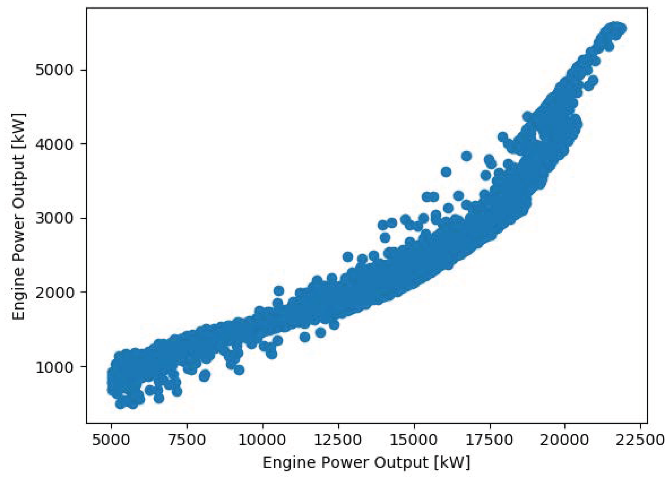
The validity of this assumption can be seen by observing Figure A1 and Figure A2 where the calculated power from the main engines is represented against the ship speed and the turbocharger speed, respectively.
where Equations (A4)–(A6) represent the mass balances of the bypass split, bypass merge, and cylinder respectively, while Equations (A7) and (A8) represent the energy balances of the turbocharger and of the bypass merge, respectively.
Figure A1.
Scatter plot, Propulsion power versus ship speed.

Figure A2.
Scatter plot, Main engine power versus turbocharger speed (ME1).
The energy balance over the whole engine is presented in Equation (A9).
with:
The value of is determined based on the balance in Equation (A9). The share between the four contributions in Equation (A13) is calculated based on the data for the heat loss to the HT and LT systems presented in the engines project guides as functions of the engine load. The values are interpolated based on a 2nd degree polynomial and scaled to respect the energy balance. In absence of more accurate data, it is then assumed that the contributions of and are equal for all loads.
The most relevant operative values are provided in Table A1 and Table A2 and the main energy flows are listed in Table A3 and Table A4.

Table A1.
Main engines, measured and calculated temperatures and flows at different engine loads.
| Variable | Unit | M/C | 30% | 50% | 70% | 90% | |
|---|---|---|---|---|---|---|---|
| Compressor | |||||||
| C | M | 302 | |||||
| C | C | 356.0 | 409.4 | 434.1 | 461.7 | ||
| kg/s | C | 4.24 | 7.62 | 8.51 | 10.28 | ||
| - | M | ||||||
| Turbine | |||||||
| C | C | 698.8 | 702.2 | 763.3 | 786.0 | ||
| C | M | 639.3 | 592.9 | 633.2 | 631.0 | ||
| kg/s | C | 4.35 | 7.79 | 8.73 | 10.57 | ||
| - | C | ||||||
| Bypass valve | |||||||
| kg/s | C | 0.98 | 2.05 | 1.02 | 0.39 | ||
| Cylinders | |||||||
| kg/s | C | 3.25 | 5.57 | 7.49 | 9.89 | ||
| kg/s | C | 0.11 | 0.17 | 0.22 | 0.28 | ||
| kg/s | C | 3.37 | 5.74 | 7.71 | 10.17 | ||
| C | M | 323.7 | 323.2 | 323.1 | 323.5 | ||
| C | M | 698.8 | 702.2 | 763.3 | 786.0 | ||
| CAC-LT stage | |||||||
| C | C | 355.2 | 350.1 | 360.0 | 368.7 | ||
| C | M | 323.7 | 323.2 | 323.1 | 323.5 | ||
| C | M | 309.3 | 309.6 | 309.5 | 309.6 | ||
| C | C | 310.4 | 311.0 | 311.8 | 313.0 | ||
| kg/s | C | 23.36 | 26.09 | 29.1 | 31.53 | ||
| CAC-HT stage | |||||||
| C | C | 356.0 | 409.4 | 434.1 | 461.7 | ||
| C | C | 355.2 | 350.1 | 360.0 | 368.7 | ||
| C | C | 360.8 | 360.2 | 359.6 | 358.7 | ||
| C | C | 360.8 | 362.6 | 363.6 | 365.4 | ||
| kg/s | C | 33.21 | 33.18 | 33.33 | 33.33 | ||
| LOC | |||||||
| C | C | 346.6 | 348.9 | 349.8 | 350.5 | ||
| C | M | 335.1 | 336.8 | 338.1 | 338.3 | ||
| C | C | 310.4 | 311.0 | 311.8 | 313.0 | ||
| C | C | 317.4 | 317.6 | 317.5 | 318.5 | ||
| JWC | |||||||
| C | C | 423 | |||||
| C | M | 358.1 | 358.4 | 357.6 | 356.4 | ||
| C | C | 360.8 | 360.2 | 359.6 | 358.7 | ||
Table A2.
Auxiliary engines, measured and calculated temperatures and flows at different engine loads.
Table A2.
Auxiliary engines, measured and calculated temperatures and flows at different engine loads.
| Variable | Unit | M/C | 30% | 50% | 70% | 90% | |
|---|---|---|---|---|---|---|---|
| Compressor | |||||||
| C | M | 284.2 | 285.3 | 284.9 | 294.6 | ||
| C | C | 323.2 | 357.9 | 391.6 | 430.9 | ||
| kg/s | C | 1.96 | 2.65 | 3.5 | 4.27 | ||
| - | M | ||||||
| Turbine | |||||||
| C | M | 729.5 | 762.1 | 770.3 | 798.5 | ||
| C | M | 652.8 | 667.8 | 654.2 | 659.4 | ||
| kg/s | C | 2.02 | 2.74 | 3.61 | 4.41 | ||
| - | C | ||||||
| Cylinders | |||||||
| kg/s | C | 1.96 | 2.65 | 3.5 | 4.27 | ||
| kg/s | C | 0.05 | 0.08 | 0.11 | 0.14 | ||
| kg/s | C | 2.02 | 2.74 | 3.61 | 4.41 | ||
| C | M | 320.8 | 322.3 | 327.6 | 329.1 | ||
| C | C | 729.5 | 762.1 | 770.3 | 798.5 | ||
| CAC-LT stage | |||||||
| C | C | 323.2 | 356.3 | 366.7 | 372.0 | ||
| C | M | 320.8 | 322.3 | 327.6 | 329.1 | ||
| C | M | 317.1 | 316.3 | 317.5 | 314.1 | ||
| C | C | 317.2 | 318.2 | 320.5 | 318.3 | ||
| kg/s | C | 11.16 | 11.16 | 10.98 | 10.78 | ||
| CAC-HT stage | |||||||
| C | C | 323.2 | 357.9 | 391.6 | 430.9 | ||
| C | C | 323.2 | 356.3 | 366.7 | 372.0 | ||
| C | C | 362.5 | 364.2 | 368.0 | 368.2 | ||
| C | C | 362.5 | 364.3 | 369.3 | 371.9 | ||
| kg/s | C | 16.66 | 16.67 | 16.55 | 16.67 | ||
| LOC | |||||||
| C | C | 348.2 | 350.3 | 354.0 | 357.3 | ||
| C | M | 336.6 | 337.4 | 339.7 | 340.4 | ||
| C | C | 317.2 | 318.2 | 320.5 | 318.3 | ||
| C | C | 325.9 | 327.8 | 331.4 | 331.3 | ||
| JWC | |||||||
| C | C | 423 | |||||
| C | M | 360.0 | 359.7 | 362.3 | 361.5 | ||
| C | C | 362.5 | 364.2 | 368.0 | 368.2 | ||
Table A3.
Main engines, energy flows at different engine loads.
| Energy Flow | Type | 30% | 50% | 70% | 90% |
|---|---|---|---|---|---|
| Power output | Mech | 1767 | 2946 | 4118 | 5293 |
| Exhaust gas (after turbine) | Heat | 1672 | 2566 | 3227 | 3938 |
| CAC-LT | Heat | 80 | 197 | 353 | 613 |
| CAC-HT | Heat | 0 | 256 | 470 | 763 |
| JWC | Heat | 501 | 507 | 549 | 620 |
| LOC | Heat | 501 | 507 | 549 | 620 |
Table A4.
Auxiliary engines, energy flows at different engine loads.
| Energy Flow | Type | 30% | 50% | 70% | 90% |
|---|---|---|---|---|---|
| Power output | Mech | 828 | 1381 | 1932 | 2482 |
| Exhaust gas (after turbine) | Heat | 808 | 1144 | 1456 | 1753 |
| CAC-LT | Heat | 5 | 92 | 139 | 185 |
| CAC-HT | Heat | 0 | 4 | 87 | 256 |
| JWC | Heat | 278 | 366 | 436 | 510 |
| LOC | Heat | 278 | 366 | 436 | 510 |
Appendix A.3. Electric Demand Modeling
Appendix A.3.1. HVAC Systems
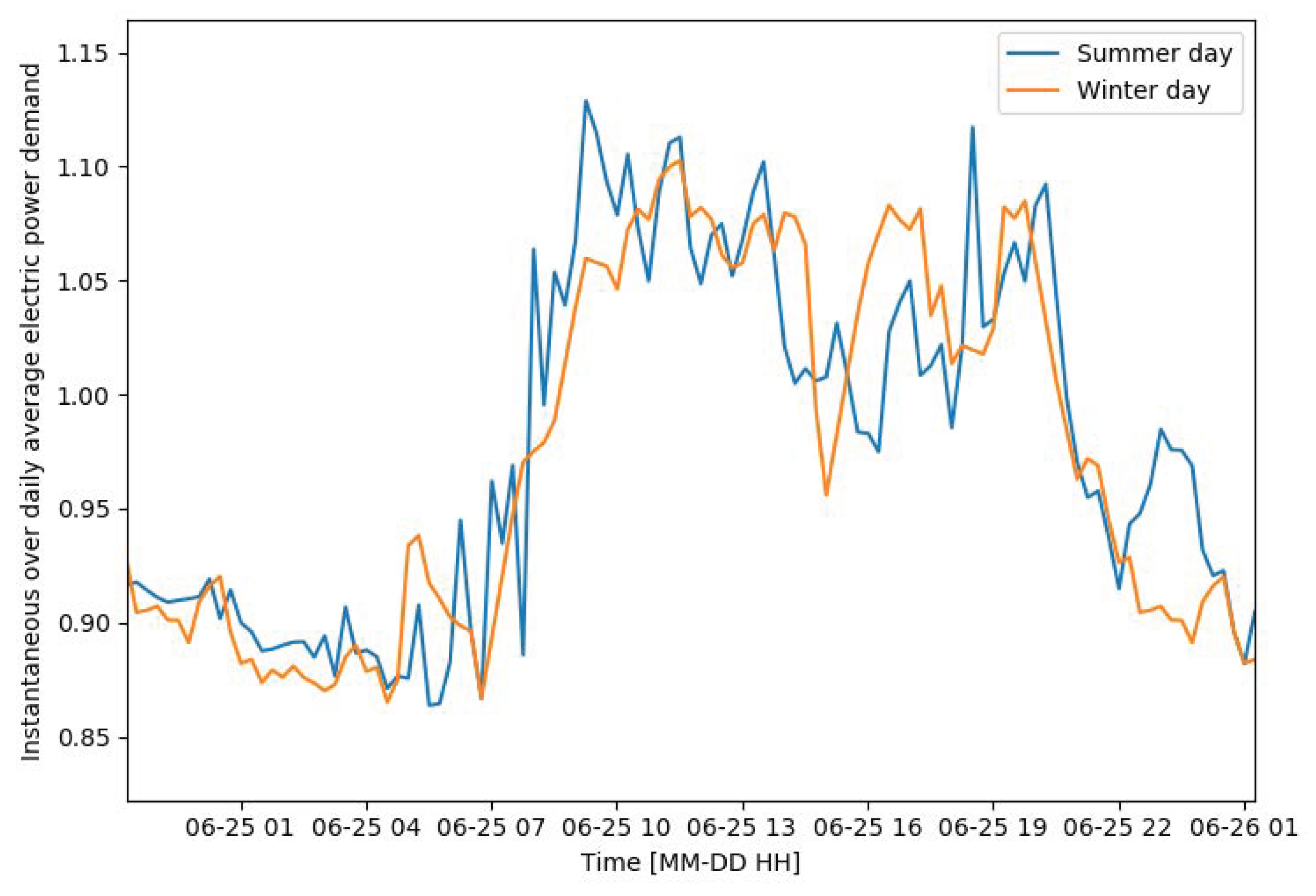
The observation of the total power demand over the year (see Figure A3, showing daily averages) leads to the identification of a period, corresponding to the summer months, when the electric power demand is significantly higher than during the remaining months. Based on this observation, in this work we assumed that the demand of the HVAC compressors related to the need for space cooling is concentrated during the summer months. Additionally, comparing the evolution of the daily demand (see Figure A4, representing the instantaneous demand divided by the daily average) between a typical summer and winter day, shows that the daily variation is comparable. This shows that assuming a constant consumption for the HVAC during the day does not introduce a substantial error in the estimations.
Figure A3.
Total electric power demand versus time (Daily average).

Figure A4.
Instantaneous power demand over daily average, winter versus summer day.
The HVAC electric power demand was estimated as follows:
where is calculated as:
Appendix A.3.2. Thrusters
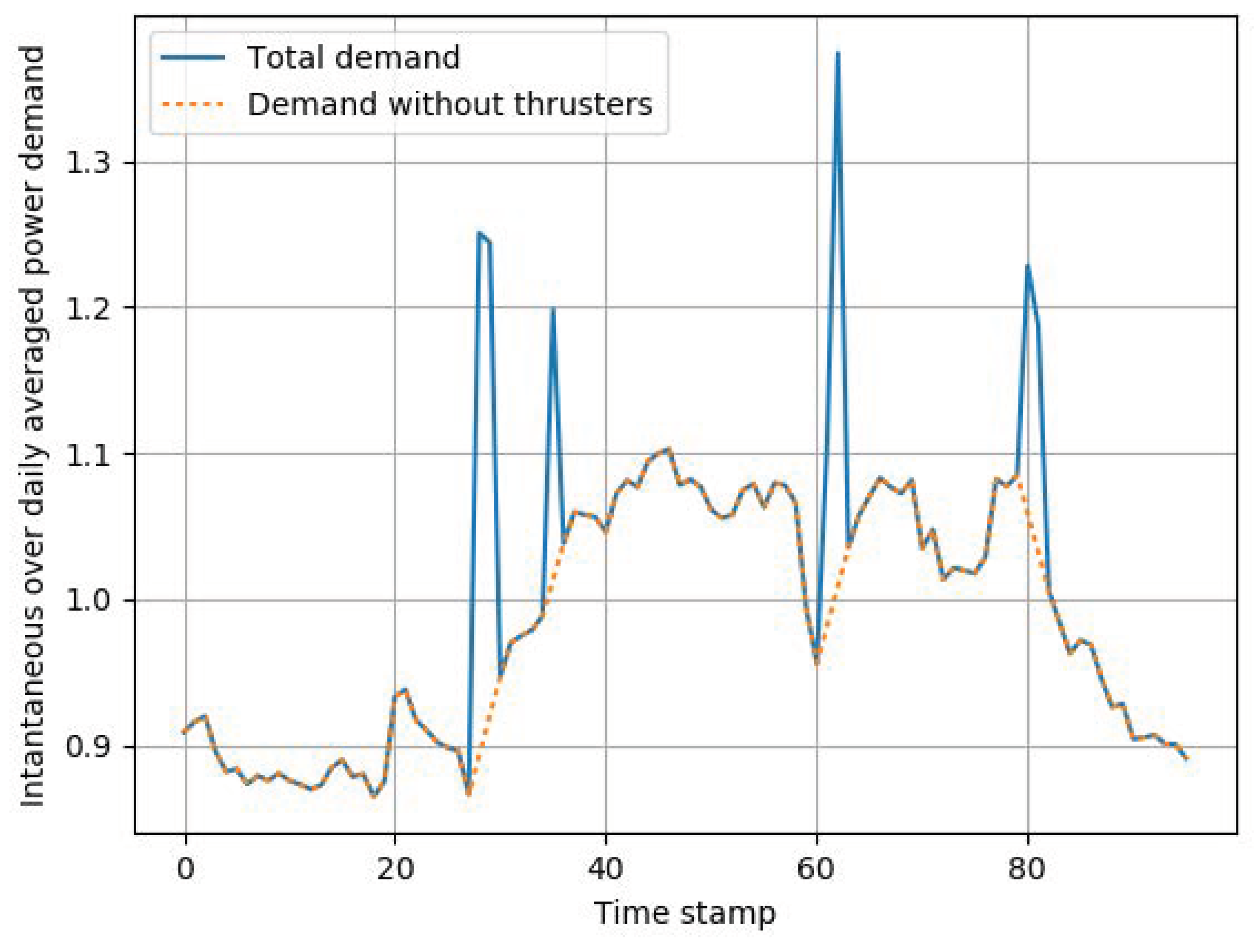
When entering port areas, the ship needs to use thrusters to maneuver and berth. In the case of this particular ships, operating on daily schedules and hence maneuvering four times per day, the power demand related to thrusters can be significant. In order to isolate the demand from the thrusters, we extracted from the ship’s operations a reference daily energy profile, based on the instantaneous electric power demand divided by the daily average. From this daily profile (made of 96 points), we manually selected the points that could be clearly identified as related to the thrusters energy demand, and substituted the actual value with a weighted average of the previous and subsequent points (see Figure A5).
By comparing the reference profile to the instantaneous one, the points where the former is more than 10% higher than the latter are identified as “thruster-on” points and treated consequently.
Figure A5.
Example of the procedure of selection of thruster power demand.
Appendix A.4. Heat Demand
The heat demand was calculated as the sum of the contributions of the elements listed in the ship’s heat balance documentation. The assumptions used in the estimation are summarized in Table A5.
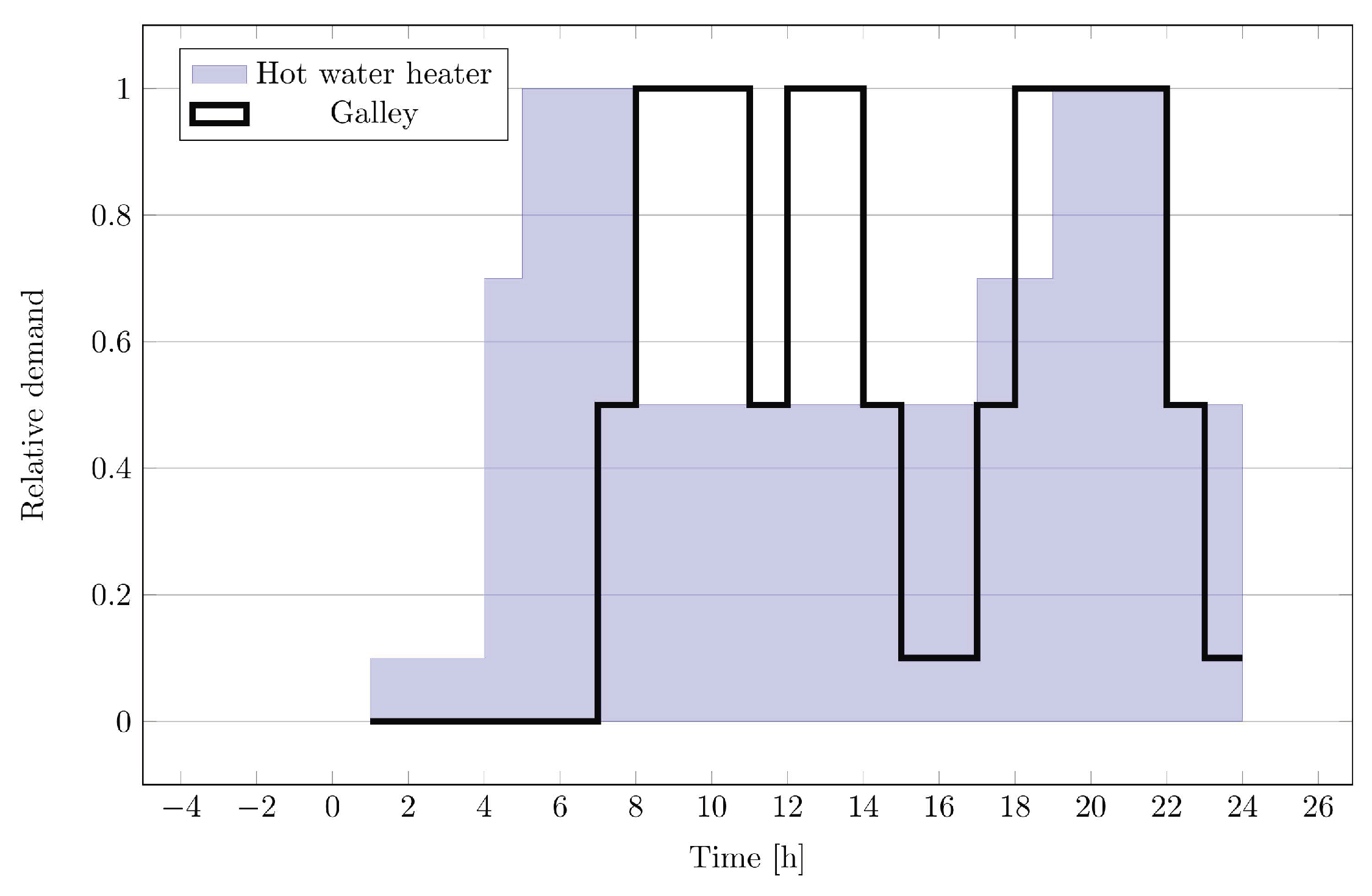
Where all factors are treated as calibration parameters (see Table A6). The and functions represent the assumption made on the daily evolution of the heating demand from the galley and the hot water heater respectively. The daily evolutions of the demand are considered to be the same over the whole year of operations and are represented graphically in Figure A6.
Figure A6.
Hourly relative demand of hot water heating and galley.

Table A5.
Summary of the heat demand contributions and their calculation.
| Heat Flow Name | Equation |
|---|---|
| HVAC Preheater | |
| HVAC Reheater | |
| Hot water heater | |
| Galley | |
| Low temperature tank heating | |
| HFO tank heating | |
| Machinery space heating | |
| HFO heater |
Appendix A.4.1. Heat Generation
The heat recovered in the EGBs is the only contribution to the heat balance that is known with a reasonable certainty. The heat transferred from the exhaust gas to the steam () is calculated according to Equation (16):
where and are measured for all EGBs, is calculated as a function of the exhaust gas composition and temperature, and is calculated based on the engine energy and mass balance.
It is known that the ship heating systems are designed for recovering energy from the high temperature cooling systems of engines on the ship. Based on the available measurements, we calculated the heat exchanged in the two HTHRs according to Equation (A18),
where the effectiveness of the heat exchanger is considered to be constant and its value is part of the parameter estimation problem (see Table A6). The HT-water outlet temperature for each engine room is calculated based on the thermal balance of the engines, and the HR water at the HTHR inlet () is considered as a calibration parameter.
The heat generated by the auxiliary boilers was calculated based on the energy balance between the heat generation and heat demand on board, i.e., to contribute with the amount of heat that cannot be provided by the waste heat recovery systems. The contribution of the boiler heat storage capacity is taken into account by a calibration parameter that determines the maximum heat deficit. This corresponds, in practice, to assuming that the boiler is started up when the steam pressure inside the boiler drops below a certain value, and stopped once the pressure has achieved its maximum operative value. In this calculation, the calibration parameters are the heat storage capacity () and the fixed heat rate () of the auxiliary boilers (see Table A6).
Appendix A.4.2. Heat Balance Parameter Estimation
The individual contributions of different consumers were determined by means of a parameter estimation procedure, using the daily boiler fuel consumption for the calibration of the parameters. The parameter estimation problem is hence written as a minimization problem:
where the vector includes the calibration parameters that are part of the heat demand and generation estimation model that is explained in detail in the following sections. A list of the parameters is shown in Table A6, together with the chosen upper and lower boundaries for the calibration procedure.
Table A6.
Parameters optimized in the parameter estimation for the heat balance.
| Parameter Name | Symbol | Unit | Lower Boundary | Higher Boundary | Optimal Value |
|---|---|---|---|---|---|
| Constant HTHR heat demand | kW | 0 | 1000 | 20.5 | |
| Constant steam demand | kW | 0 | 1000 | 0 | |
| Weight factor of the HVAC Re-heater | - | 0.5 | 1 | 0.40 | |
| Weight factor of the HVAC Pre-heater | - | 0 | 1 | 1.00 | |
| Weight factor of hot water heater | - | 0.5 | 1 | 0.72 | |
| Weight factor of the galley | - | 0.5 | 1 | 0.68 | |
| Weight factor of the other consumers | - | 0.5 | 1 | 0.21 | |
| HTHR inlet temperature | K | 343 | 353 | 348 | |
| Effectiveness of the HTHR HEX | - | 0.5 | 0.9 | 0.5 | |
| Boiler drum steam storage capacity | MJ | 100 | 100,000 | 9.5 × | |
| Boiler heat rate | kW | 2000 | 8000 | 5100 |
Appendix A.4.3. Uncertainty Quantification of Heat Demand
In this study, we base the estimation of the uncertainty on the production side, as it is the one that has the largest amount of information available. In these regards, the uncertainty can be reduced to the contribution of three elements: , , .
The uncertainty on the heat generated in the EGBs can be further subdivided based on its definition as a composition of the uncertainty of , , , and . In the case of and , measured values are used, where the uncertainty is related to the sensors (K-type thermocouples) that can be as high as 4% [CIT]. The uncertainty on the is related to the calculation assumptions and can be estimated of being up to 10%. The uncertainty of the value, given that both composition and temperature are accounted for, should be within 5% of the reference value. These assumptions lead to the following estimation of the uncertainty:
The resulting uncertainty can be as high as 30%, where most of the variability is related to the temperature measurements.
The uncertainty of the heat generated by the ABs can be reduced to the contribution of two elements: the uncertainty on and that on . The former will be at least as large as the calibration error (35%) and will be considered equal to 50% to be conservative and accounting also for errors in the aggregated boiler fuel measurements. In addition, the uncertainty on the efficiency can be considered to be around 10% based on the discrepancy between the considered sources and on the expected variability of the efficiency with load. As with the previous case, the combination of these efficiencies lead to a total uncertainty of 51%, where the main contribution comes from the uncertainty of the model output compared to the actual fuel consumption.
The estimation of the uncertainty of can be based on Equation (A18) having assigned an acceptable variation of 20% to the effectiveness of the heat exchanger, 20% on the estimation of the reference mass flow, K uncertainty on water temperature measurements and considering negligible the uncertainty on , leading to a 145% uncertainty on this measurement.
Appendix A.5. Full List of Exchangers in the Ship’s Heat Exchanger Network
Table A7.
Full list of exchangers in the ship’s heat exchanger networks.
| Identifier | Full Name | |
|---|---|---|
| Low temperature cooling | Charge air cooler, LT stage (ME1) | |
| Lubricating oil cooler (ME1) | ||
| Charge air cooler, LT stage (ME3) | ||
| Lubricating oil cooler (ME3) | ||
| Charge air cooler, LT stage (AE1) | ||
| Lubricating oil cooler (AE1) | ||
| Charge air cooler, LT stage (AE3) | ||
| Lubricating oil cooler (AE3) | ||
| Generator cooler (AE) | ||
| Propeller oil cooler | ||
| Shaft bearing cooler (ME) | ||
| Steam condenser | ||
| Fin stabiliser cooler | ||
| Gearbox cooler | ||
| High temperature cooling | Jacket water cooler (ME1) | |
| Charge air cooler, HT stage (ME1) | ||
| Jacket water cooler (ME3) | ||
| Charge air cooler, HT stage (ME3) | ||
| Jacket water cooler (AE1) | ||
| Charge air cooler, HT stage (AE1) | ||
| Jacket water cooler (AE3) | ||
| Charge air cooler, HT stage (AE3) | ||
| Heat recovery from HT cooling (eng.room1/3) | ||
| Hot water heat recovery system | Heat recovery from HT cooling (eng.room1/3) | |
| Heat recovery from HT cooling (eng.room 2/4) | ||
| Steam heater | ||
| AC-Reating | ||
| AC-Preheating | ||
| Hot water heater | ||
| Technical water generator | ||
| Steam systems | Heat recovery steam generator (AE1) | |
| Heat recovery steam generator (AE3) | ||
| Heat recovery steam generator (ME3) | ||
| Heat recovery steam generator (AE2) | ||
| Heat recovery steam generator (AE4) | ||
| Heat recovery steam generator (ME2) | ||
| Auxiliary boiler 1 | ||
| Auxiliary boiler 2 |
References
- IPCC. Climate Change 2014: Synthesis Report. Contribution of Working Groups I, II and III to the Fifth Assessment Report of the Intergovernamental Panel on Climate Change; Core Writing Team, Pachauri, R.K., Meyer, L.A., Eds.; Synthesis Report; IPCC: Geneva, Switzerland, 2014. [Google Scholar]
- Smith, T.; Jalkanen, J.P.; Anderson, B.; Corbett, J.J.; Faber, J.S.H.; O’Keeffe, E.; Parker, S.; Johansson, L.; Aldous, L.; Raucci, C.; et al. Third IMO GHG Study; Technical Report; International Maritime Organization (IMO): London, UK, 2014. [Google Scholar]
- Taljegard, M.; Brynolf, S.; Grahn, M.; Andersson, K.; Johnson, H. Cost-effective choices of marine fuels in a carbon-constrained world: results from a global energy model. Environ. Sci. Technol. 2014, 48, 12986–12993. [Google Scholar] [CrossRef] [PubMed]
- Sadeghinezhad, E.; Kazi, S.; Sadeghinejad, F.; Badarudin, A.; Mehrali, M.; Sadri, R.; Reza Safaei, M. A comprehensive literature review of bio-fuel performance in internal combustion engine and relevant costs involvement. Renew. Sustain. Energy Rev. 2014, 30, 29–44. [Google Scholar] [CrossRef]
- Andersson, K.; Brynolf, S.; Lindgren, J.F.; Wilewska-Bien, M. Shipping and the Environment; Springer: Berlin, Germany, 2016. [Google Scholar]
- MEPC. Meeting Summary of the Marine Environment Protection Committee (MEPC), 72nd Session. Available online: http://www.imo.org/en/MediaCentre/MeetingSummaries/MEPC/Pages/MEPC-72nd-session.aspx (accessed on 6 August 2018).
- CLIA. 2018 Cruise Industry Outlook; Technical Report; Cruise Lines International Association: Washington, DC, USA, 2017. [Google Scholar]
- Eijgelaar, E.; Thaper, C.; Peeters, P. Antarctic cruise tourism: The paradoxes of ambassadorship, “last chance tourism” and greenhouse gas emissions. J. Sustain. Tour. 2010, 18, 337–354. [Google Scholar] [CrossRef]
- Brynolf, S.; Baldi, F.; Johnson, H. Energy Efficiency and Fuel Changes to Reduce Environmental Impacts. In Shipping and the Environment; Springer: Berlin, Germany, 2016. [Google Scholar]
- Bouman, E.A.; Lindstad, E.; Rialland, A.I.; Strømman, A.H. State-of-the-art technologies, measures, and potential for reducing GHG emissions from shipping—A review. Transp. Res. Part D-Transp. Environ. 2017, 52, 408–421. [Google Scholar] [CrossRef]
- Shi, W.; Stapersma, D.; Grimmelius, H.T. Analysis of energy conversion in ship propulsion system in off-design operation conditions. WIT Trans. Ecol. Environ. 2009, 121, 449–460. [Google Scholar] [CrossRef]
- Theotokatos, G.; Tzelepis, V. A computational study on the performance and emission parameters mapping of a ship propulsion system. Proc. Inst. Mech. Eng. Part M J. Eng. Marit. Environ. 2015, 229, 58–76. [Google Scholar] [CrossRef]
- Martelli, M.; Vernengo, G.; Bruzzone, D.; Notti, E. Holistic modeling of the global propulsion energy index in waves for small craft. Int. J. Offshore Polar Eng. 2017, 27, 442–447. [Google Scholar] [CrossRef]
- Jafarzadeh, S.; Pedersen, E.; Notti, E.; Sala, A.; Ellingsen, H. A bond graph approach to improve the energy efficiency of ships. In Proceedings of the ASME 2014 33rd International Conference on Ocean, Offshore and Arctic Engineering, San Francisco, CA, USA, 8–13 June 2014; Volume 8B. [Google Scholar] [CrossRef]
- Yan, X.; Sun, X.; Yin, Q. Multiparameter sensitivity analysis of operational energy efficiency for inland river ships based on backpropagation neural network method. Mar. Technol. Soc. J. 2016, 49, 148–153. [Google Scholar] [CrossRef]
- Yuan, Y.; Li, Z.; Malekian, R.; Yan, X. Analysis of the operational ship energy efficiency considering navigation environmental impacts. J. Mar. Eng. Technol. 2017, 16, 150–159. [Google Scholar] [CrossRef]
- Galli, A.M.; Gualeni, P.; Stranieri, G.; Qualitch, S.; Cusano, G. Monitoring and analysis of the performance data of a RO-PAX ship in the perspective of energy efficiency. Pol. Mar. Res. 2014, 21, 18–26. [Google Scholar] [CrossRef]
- Thomas, G.; O’Doherty, D.; Sterling, D.; Chin, C. Energy audit of fishing vessels. Proc. Inst. Mech. Eng. Part M J. Eng. Marit. Environ. 2010, 224, 87–101. [Google Scholar] [CrossRef]
- Buglioni, G.; Notti, E.; Sala, A. E-audit: Energy use in Italian fishing vessels. In Sustainable Maritime Transportation and Exploitation of Sea Resources; CRC Press: Boca Raton, FL, USA, 2011; Volume 2, pp. 1043–1047. [Google Scholar]
- Basurko, O.C.; Gabiña, G.; Uriondo, Z. Energy performance of fishing vessels and potential savings. J. Clean. Prod. 2013, 54, 30–40. [Google Scholar] [CrossRef]
- Parker, R.; Tyedmers, P. Fuel consumption of global fishing fleets: Current understanding and knowledge gaps. Fish Fish. 2015, 16, 684–696. [Google Scholar] [CrossRef]
- Parker, R.; Gardner, C.; Green, B.; Hartmann, K.; Watson, R. Drivers of fuel use in rock lobster fisheries. ICES J. Mar. Sci. 2017, 74, 1681–1689. [Google Scholar] [CrossRef]
- Coraddu, A.; Figari, M.; Savio, S. Numerical investigation on ship energy efficiency by Monte Carlo simulation. Proc. Inst. Mech. Eng. Part M J. Eng. Marit. Environ. 2014, 228, 220–234. [Google Scholar] [CrossRef]
- Simonsen, M.; Walnum, H.J.; Gössling, S. Model for Estimation of Fuel Consumption of Cruise Ships. Energies 2018, 11, 1059. [Google Scholar] [CrossRef]
- Baldi, F.; Johnson, H.; Gabrielii, C.; Andersson, K. Energy and exergy analysis of ship energy systems—The case study of a chemical tanker. Int. J. Thermodyn. 2015, 18, 82–93. [Google Scholar] [CrossRef]
- Marty, P.; Corrignan, P.; Gondet, A.; Chenouard, R.; Hétet, J. Modelling of energy flows and fuel consumption on board ships: Application to a large modern cruise vessel and comparison with sea monitoring data. In Proceedings of the 11th International Marine Design Conference, Glasgow, UK, 11–14 June 2012. [Google Scholar]
- Shu, G.; Liang, Y.; Wei, H.; Tian, H.; Zhao, J.; Liu, L. A review of waste heat recovery on two-stroke IC engine aboard ships. Renew. Sustain. Energy Rev. 2013, 19, 385–401. [Google Scholar] [CrossRef]
- Mondejar, M.; Andreasen, J.; Pierobon, L.; Larsen, U.; Thern, M.; Haglind, F. A review of the use of organic Rankine cycle power systems for maritime applications. Renew. Sustain. Energy Rev. 2018, 91, 126–151. [Google Scholar] [CrossRef]
- Mondejar, M.E.; Ahlgren, F.; Thern, M.; Genrup, M. Quasi-steady state simulation of an organic Rankine cycle for waste heat recovery in a passenger vessel. Appl. Energy 2017, 185, 1324–1335. [Google Scholar] [CrossRef]
- Baldi, F.; Ahlgren, F.; Melino, F.; Gabrielii, C.; Andersson, K. Optimal load allocation of complex ship power plants. Energy Convers. Manag. 2016, 124, 344–356. [Google Scholar] [CrossRef]
- SMHI. Explorer SMHIs Data. Online Resource. Available online: http://opendata-catalog.smhi.se/explore/ (accessed on 7 August 2018).
- Bejan, A.; Tsatsaronis, G.; Moran, M. Thermal Design and Optimization; John Wiley & Sons: Hoboken, NJ, USA, 1996. [Google Scholar]
- Kotas, T.J. The Exergy Method of Thermal Plant Analysis; Elsevier: New York, NY, USA, 2013. [Google Scholar]
- Tsatsaronits, G. Definitions and nomenclature in exergy analysis and exergoeconomics. Energy 2007, 32, 249–253. [Google Scholar] [CrossRef]
- Szargut, J. Chemical exergies of the elements. Appl. Energy 1989, 32, 269–286. [Google Scholar] [CrossRef]
- Tsatsaronis, G. Thermoeconomic analysis and optimization of energy systems. Prog. Energy Combust. Sci. 1993, 19, 227–257. [Google Scholar] [CrossRef]
- Kanungo, T.; Mount, D.M.; Netanyahu, N.S.; Piatko, C.D.; Silverman, R.; Wu, A.Y. An efficient k-means clustering algorithm: Analysis and implementation. IEEE Trans. Pattern Anal. Mach. Intell. 2002, 24, 881–892. [Google Scholar] [CrossRef]
- Fazlollahi, S.; Bungener, S.L.; Mandel, P.; Becker, G.; Maréchal, F. Multi-objectives, multi-period optimization of district energy systems: I. Selection of typical operating periods. Comput. Chem. Eng. 2014, 65, 54–66. [Google Scholar] [CrossRef] [Green Version]
- Keogh, E.; Chakrabarti, K.; Pazzani, M.; Mehrotra, S. Locally adaptive dimensionality reduction for indexing large time series databases. ACM Sigmod. Rec. 2001, 30, 151–162. [Google Scholar] [CrossRef] [Green Version]
- Baldi, F.; Maréchal, F.; Tammi, K. Process integration as a tool for the improvement of cruise ships energy efficiency. In Proceedings of the Shipping in Changing Climate Conference, London, UK, 4–5 September 2017. [Google Scholar]
- Ahlgren, F.; Mondejar, M.E.; Genrup, M.; Thern, M. Waste heat recovery in a cruise vessel in the Baltic Sea by using an Organic Rankine Cycle: A case study. J. Eng. Gas Turbines Power 2016, 138, 011702. [Google Scholar] [CrossRef]
- Sakalis, G.N.; Frangopoulos, C.A. Intertemporal optimization of synthesis, design and operation of integrated energy systems of ships: General method and application on a system with Diesel main engines. Appl. Energy 2018, 226, 991–1008. [Google Scholar] [CrossRef]
- Trivyza, N.L.; Rentizelas, A.; Theotokatos, G. A novel multi-objective decision support method for ship energy systems synthesis to enhance sustainability. Energy Convers. Manag. 2018, 168, 128–149. [Google Scholar] [CrossRef]
- Banks, C.; Turan, O.; Incecik, A.; Theotokatos, G.; Izkan, S.; Shewell, C.; Tian, X. Understanding Ship Operating Profiles with an Aim to Improve Energy Efficient Ship Operations. In Proceedings of the Low Carbon Shipping Conference, London, UK, 9–10 September 2013; pp. 1–11. [Google Scholar]
- Bock, H.G. (Ed.) Model Based Parameter Estimation: Theory and Applications; Number v.4 in Contributions in Mathematical and Computational Sciences; Springer: Berlin, Germany; New York, NY, USA, 2013. [Google Scholar]
- Crowe, C.M. Data reconciliation—Progress and challenges. J. Process Control 1996, 6, 89–98. [Google Scholar] [CrossRef]
- McKinney, W. Data Structures for Statistical Computing in Python. In Proceedings of the 9th Python in Science Conference, Austin, TX, USA, 28–30 June 2010; pp. 51–56. [Google Scholar]
Figure 1.
Reference operational profile (ship speed vs. time) for the case study. The two-way voyage from Stockholm to Mariehamn typically includes two stops in port, one period of stationing at sea during night, and two main sailing parts.
Figure 1.
Reference operational profile (ship speed vs. time) for the case study. The two-way voyage from Stockholm to Mariehamn typically includes two stops in port, one period of stationing at sea during night, and two main sailing parts.
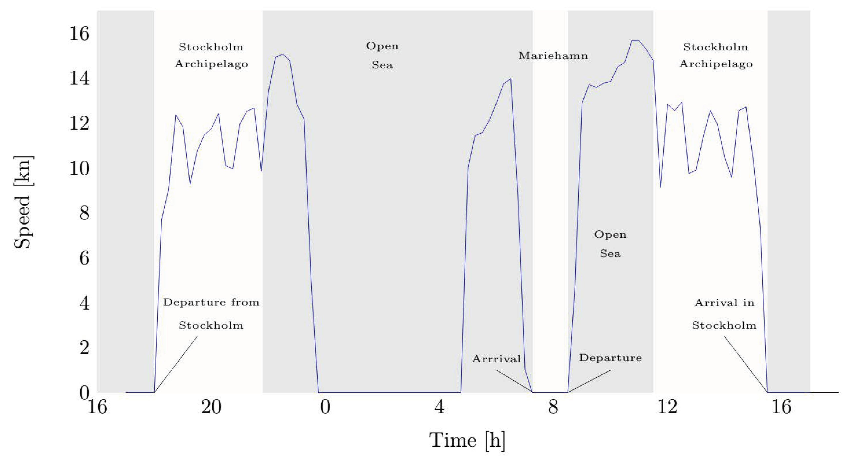
Figure 2.
Layout of the energy system of the case study. Energy converters are listed on the left, while the energy demands are summarized on the right. The blue, red and green colors refer to electric power, heat, and mechanical power, respectively.
Figure 2.
Layout of the energy system of the case study. Energy converters are listed on the left, while the energy demands are summarized on the right. The blue, red and green colors refer to electric power, heat, and mechanical power, respectively.
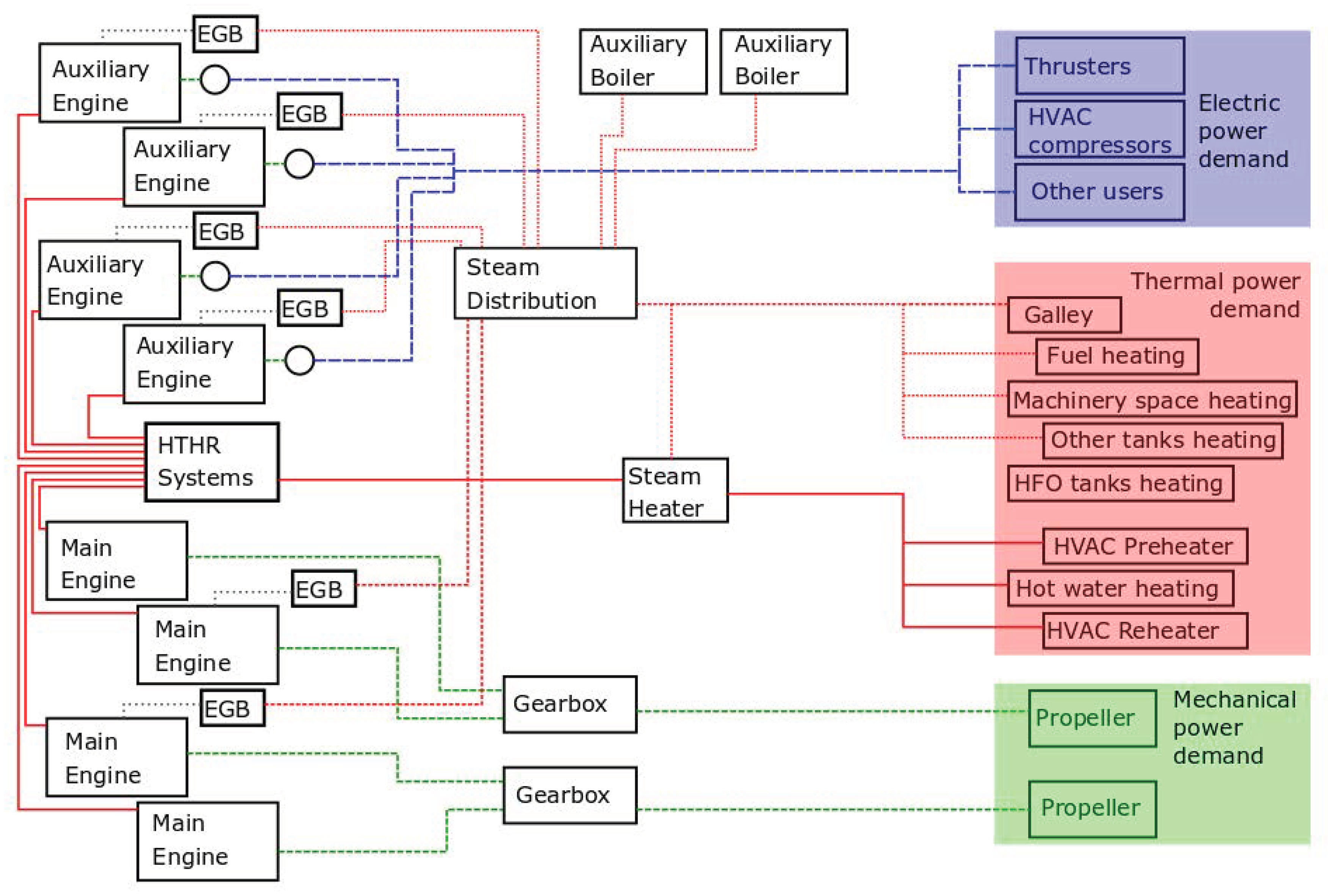
Figure 3.
Overview of the method, including the inputs coming from the data collection, the data processing, and the outputs of the energy and exergy analysis.
Figure 3.
Overview of the method, including the inputs coming from the data collection, the data processing, and the outputs of the energy and exergy analysis.

Figure 4.
Schematic representation of the Diesel engines and of their connections to the cooling systems.
Figure 4.
Schematic representation of the Diesel engines and of their connections to the cooling systems.

Figure 5.
General view of the ship heating and cooling systems. The full list of heat exchangers in the heat exchanger network is provided in Appendix A.5 in Table A7.
Figure 5.
General view of the ship heating and cooling systems. The full list of heat exchangers in the heat exchanger network is provided in Appendix A.5 in Table A7.
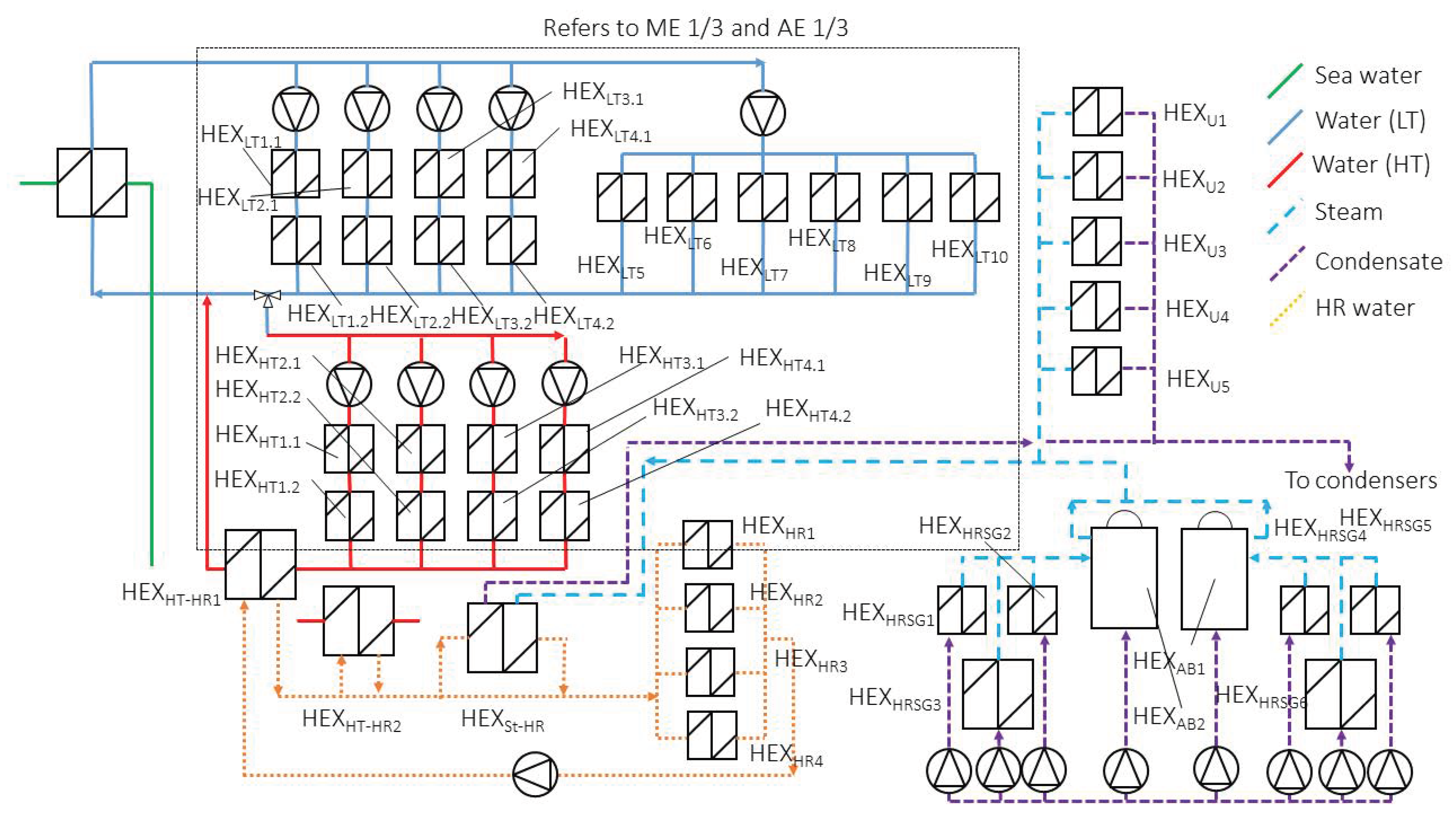
Figure 6.
Measured air and sea water temperatures based on yearly data for the investigated period of ship operations. Landsort, 2014.
Figure 6.
Measured air and sea water temperatures based on yearly data for the investigated period of ship operations. Landsort, 2014.

Figure 7.
Yearly distribution of ship speed. Periods spent in port at 0 speed are excluded from the count.
Figure 7.
Yearly distribution of ship speed. Periods spent in port at 0 speed are excluded from the count.

Figure 8.
Share of time spent by the ship in each operational mode considered in the analysis.
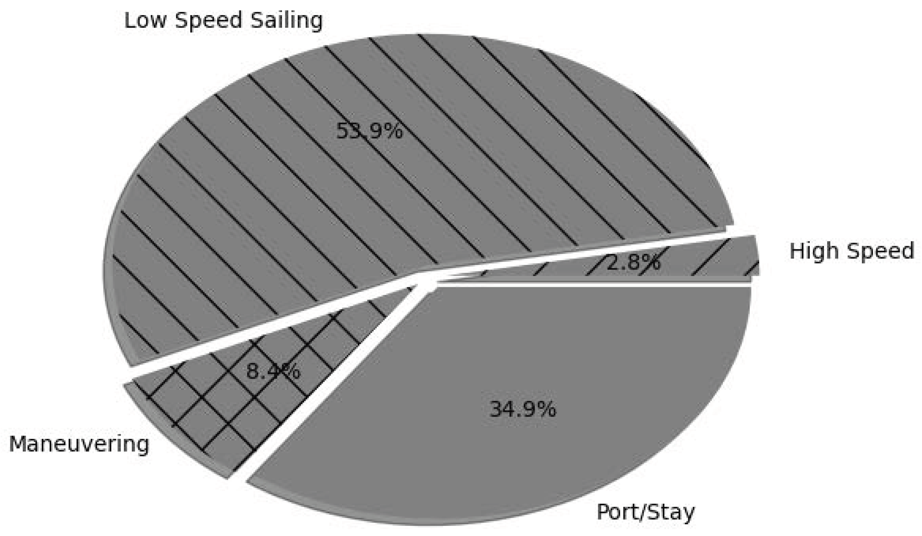
Figure 9.
Yearly load distribution of the ship’s main engines.
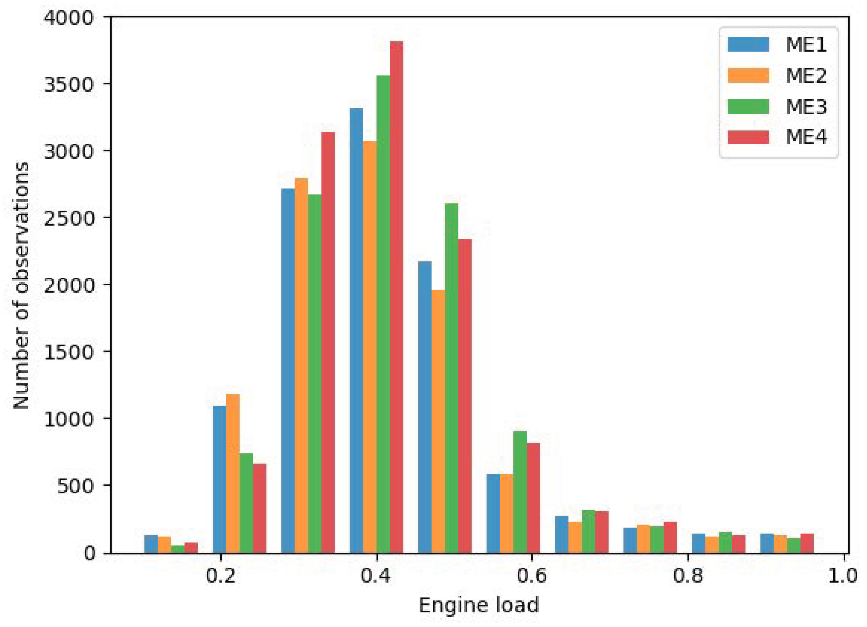
Figure 10.
Yearly load distribution of the ship’s auxiliary engines.

Figure 11.
Energy demand during a day of operations, Winter (31 January).

Figure 12.
Energy demand during a day of operations, Summer (31 July).

Figure 13.
Total ship energy demand subdivided by user, aggregated data for one year of operations. Green and blue areas refer to mechanical and electric power, respectively. Orange and red refer to low- and high-temperature heat demand, respectively.
Figure 13.
Total ship energy demand subdivided by user, aggregated data for one year of operations. Green and blue areas refer to mechanical and electric power, respectively. Orange and red refer to low- and high-temperature heat demand, respectively.
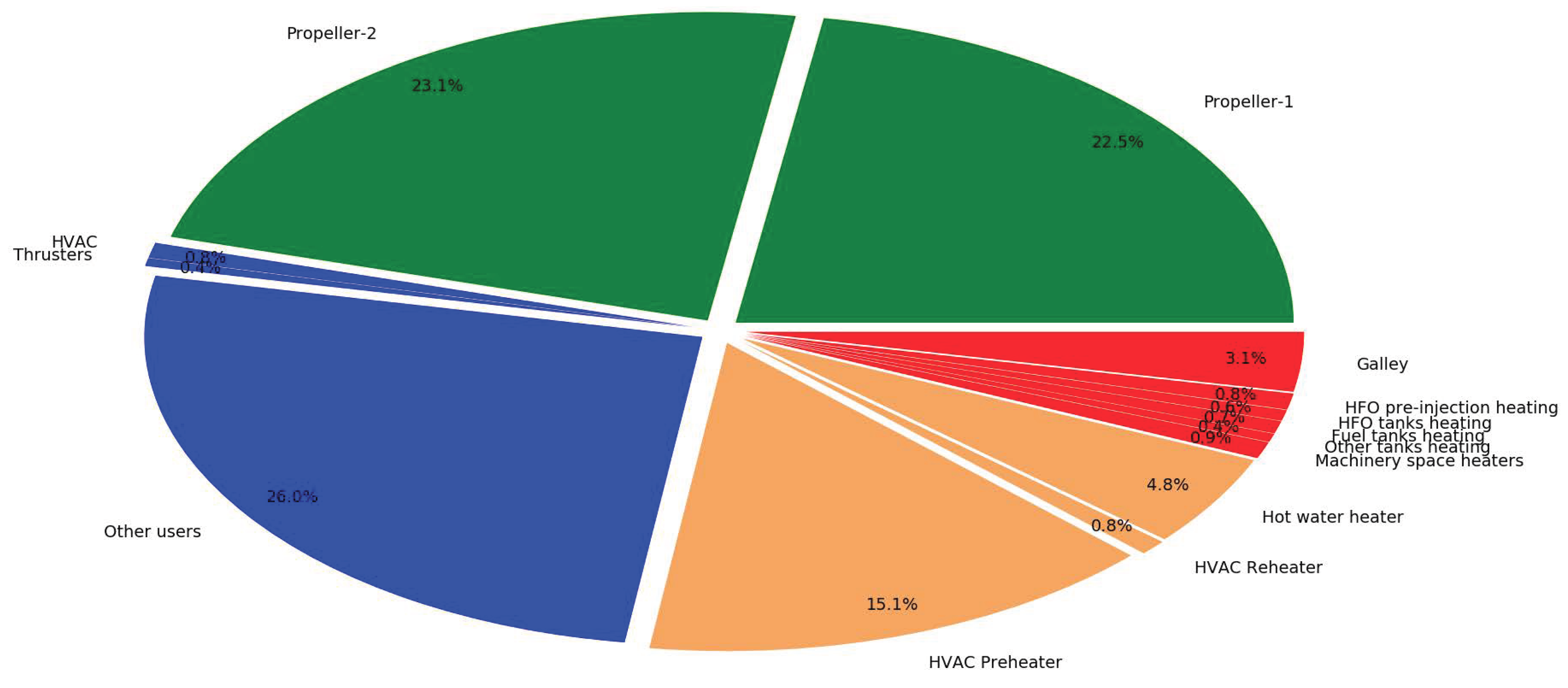
Figure 14.
Share of thermal power generated from on-board heat systems, aggregated values for one year of ship. White refers to the auxiliary boilers, light gray to the hot water heat recovery systems, dark gray to heat recovery steam generators.
Figure 14.
Share of thermal power generated from on-board heat systems, aggregated values for one year of ship. White refers to the auxiliary boilers, light gray to the hot water heat recovery systems, dark gray to heat recovery steam generators.

Figure 15.
Total ship energy generation for each engine/boiler, aggregated data for one year of operations. Light gray refers to auxiliary engines, dark gray to main engines, and black to the auxiliary boilers.
Figure 15.
Total ship energy generation for each engine/boiler, aggregated data for one year of operations. Light gray refers to auxiliary engines, dark gray to main engines, and black to the auxiliary boilers.
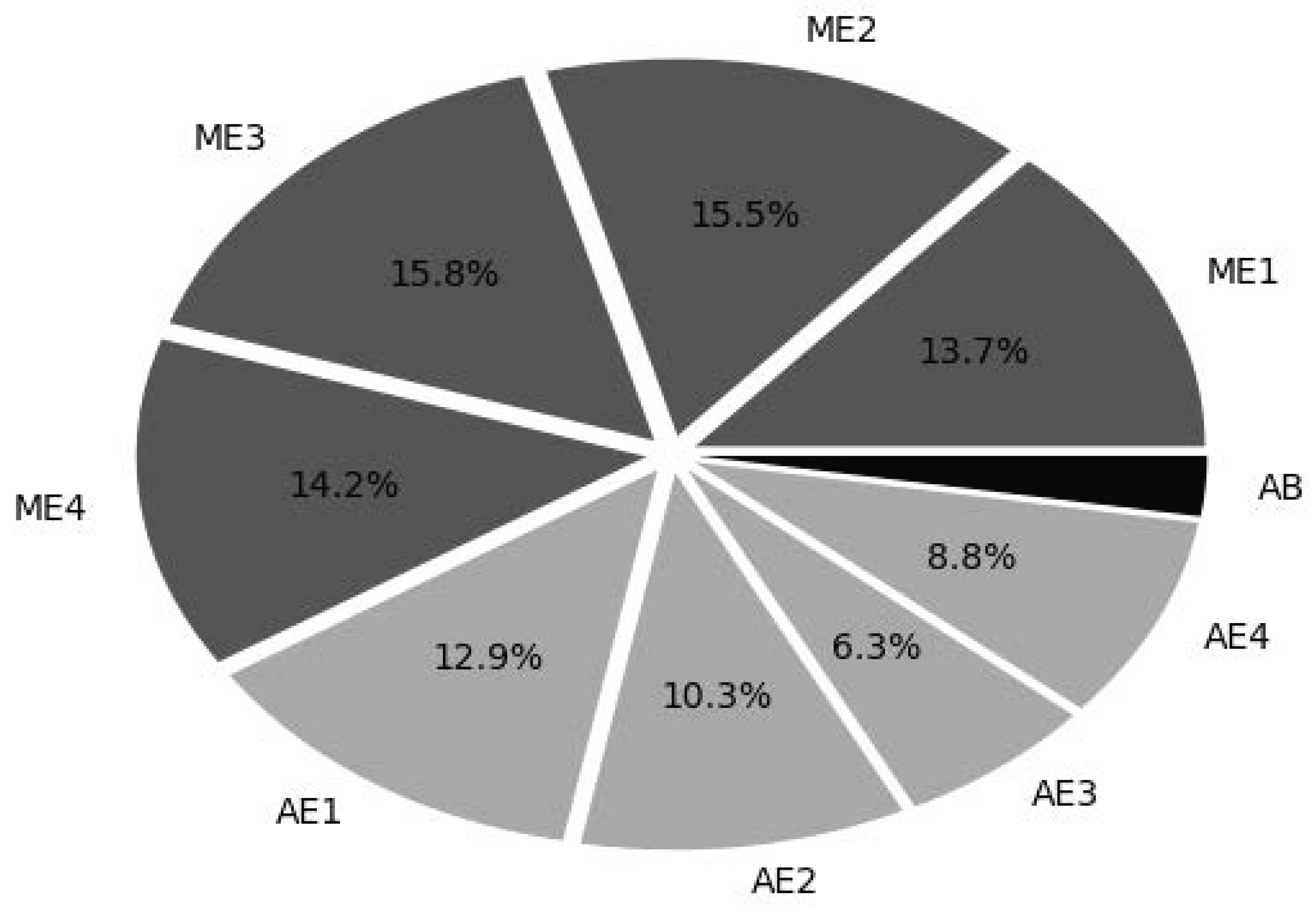
Figure 16.
Time series representation of the thermal power generated from on-board heat systems.

Figure 17.
Sankey diagram. The purple color refers to chemical energy; the green color refers to electric/mechanical energy. The yellow color refers to the exergy in the exhaust gas; the orange color refers to the energy in the cooling flows; the red color refers to the energy losses. Flow values are in GWh/year.
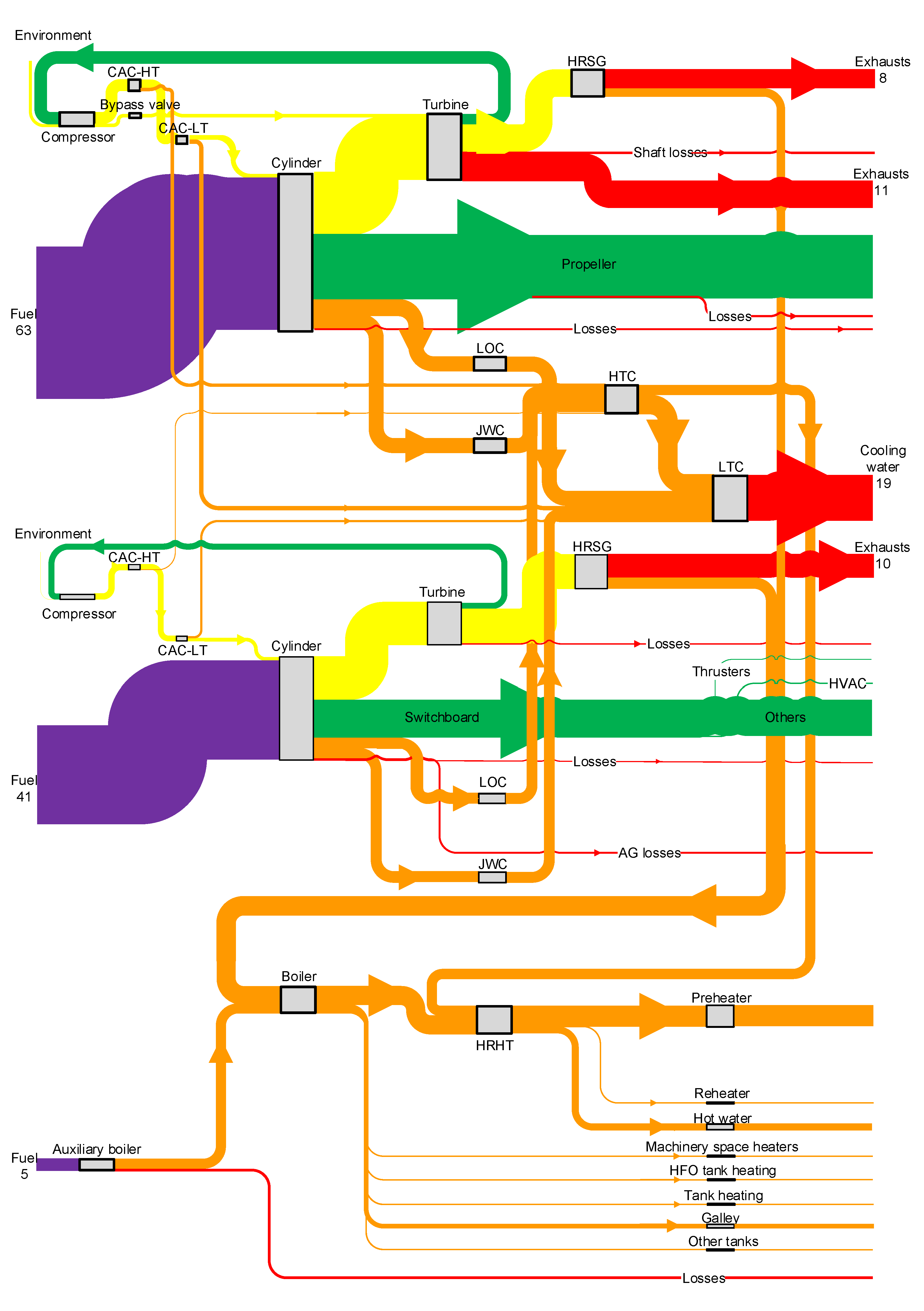
Figure 18.
Grassmann diagram. The purple color refers to chemical exergy; the green color refers to electric/mechanical exergy. The yellow color refers to the exergy in the exhaust gas; the orange color refers to the exergy in the cooling flows; the red color refers to the energy losses. The exergy destruction is not represented to preserve the readability of the diagram. Flow values are in GWh/year.
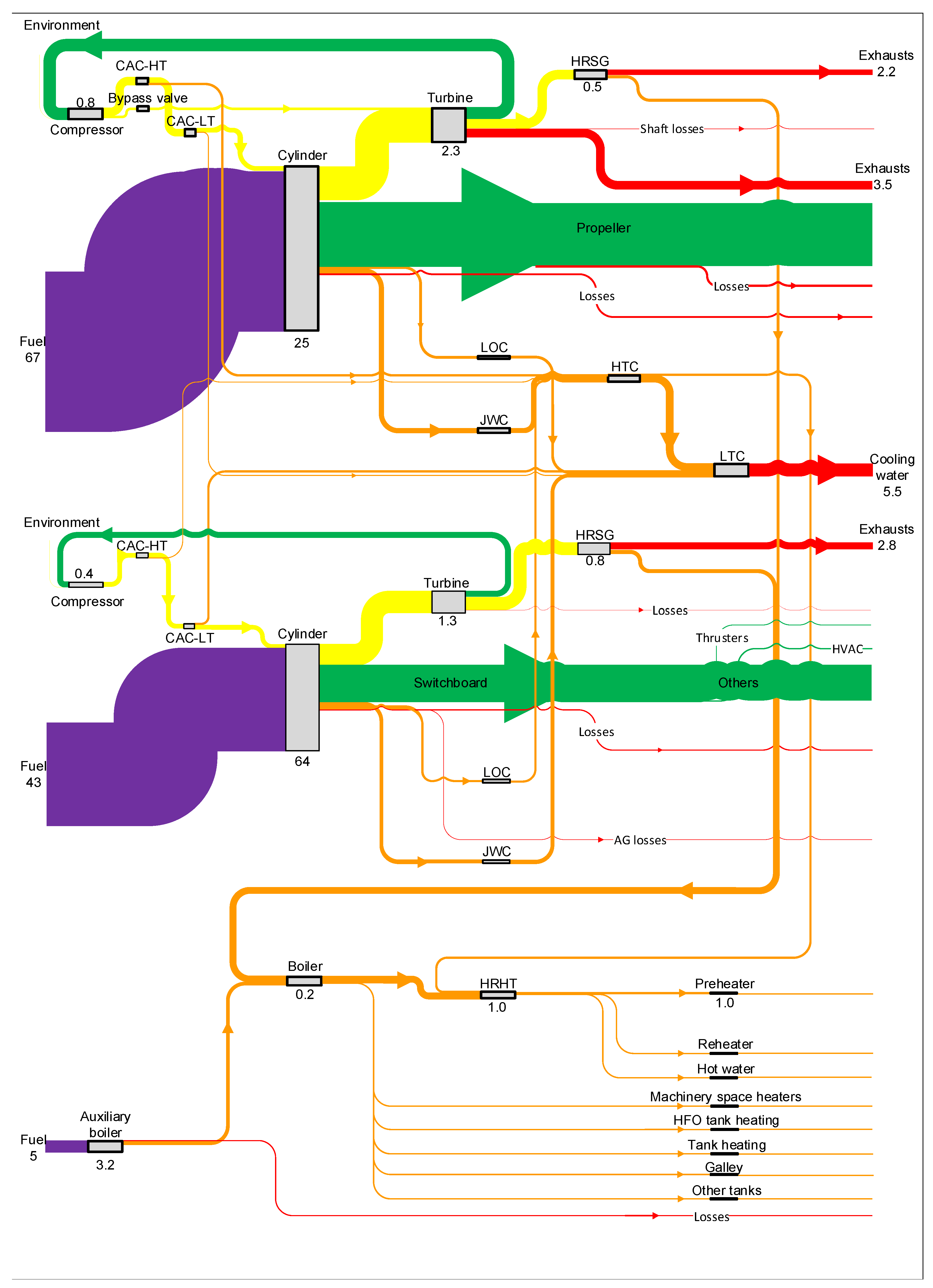
Figure 19.
Energy and exergy efficiency of the WHR systems.
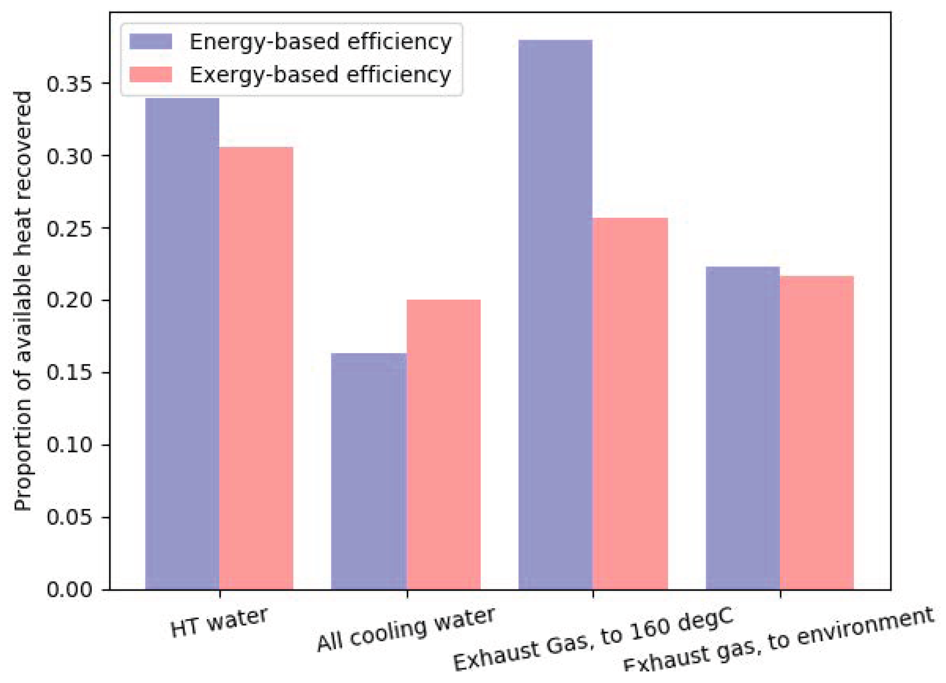
Figure 20.
Power profile and duration curves, represented with the 35,040 datapoints (black curve) and five typical days (other colors).
Figure 20.
Power profile and duration curves, represented with the 35,040 datapoints (black curve) and five typical days (other colors).
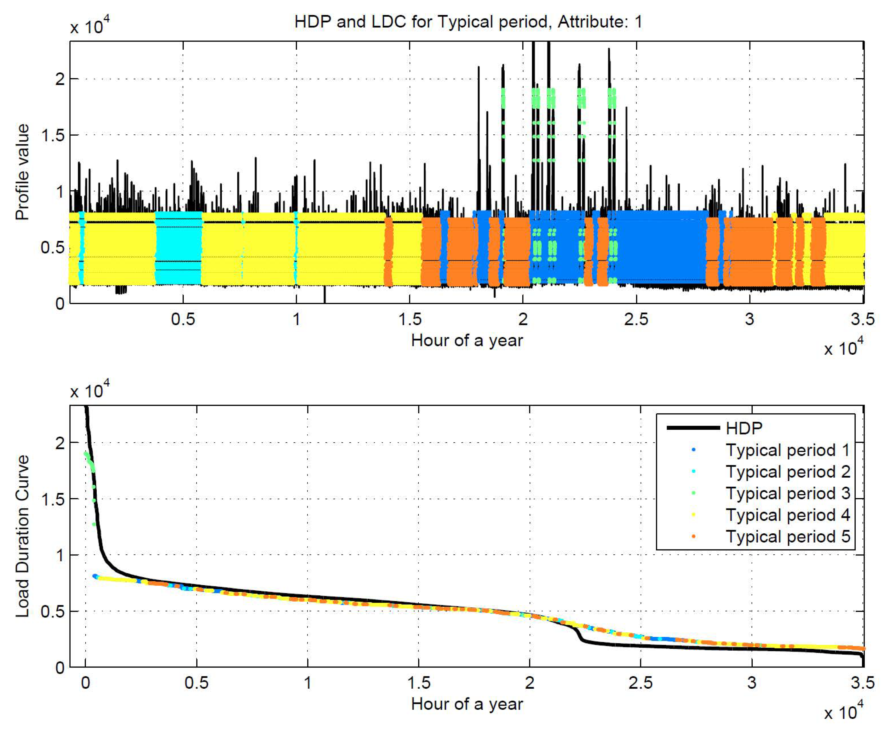
Figure 21.
Power profile and duration curves, represented with the 35,040 datapoints (black curve) and five typical days (other colors).
Figure 21.
Power profile and duration curves, represented with the 35,040 datapoints (black curve) and five typical days (other colors).

Figure 22.
Power (left) and heat (right) profiles, original (green) and segmented (blue), for the 5 typical days and duration curves.
Figure 22.
Power (left) and heat (right) profiles, original (green) and segmented (blue), for the 5 typical days and duration curves.
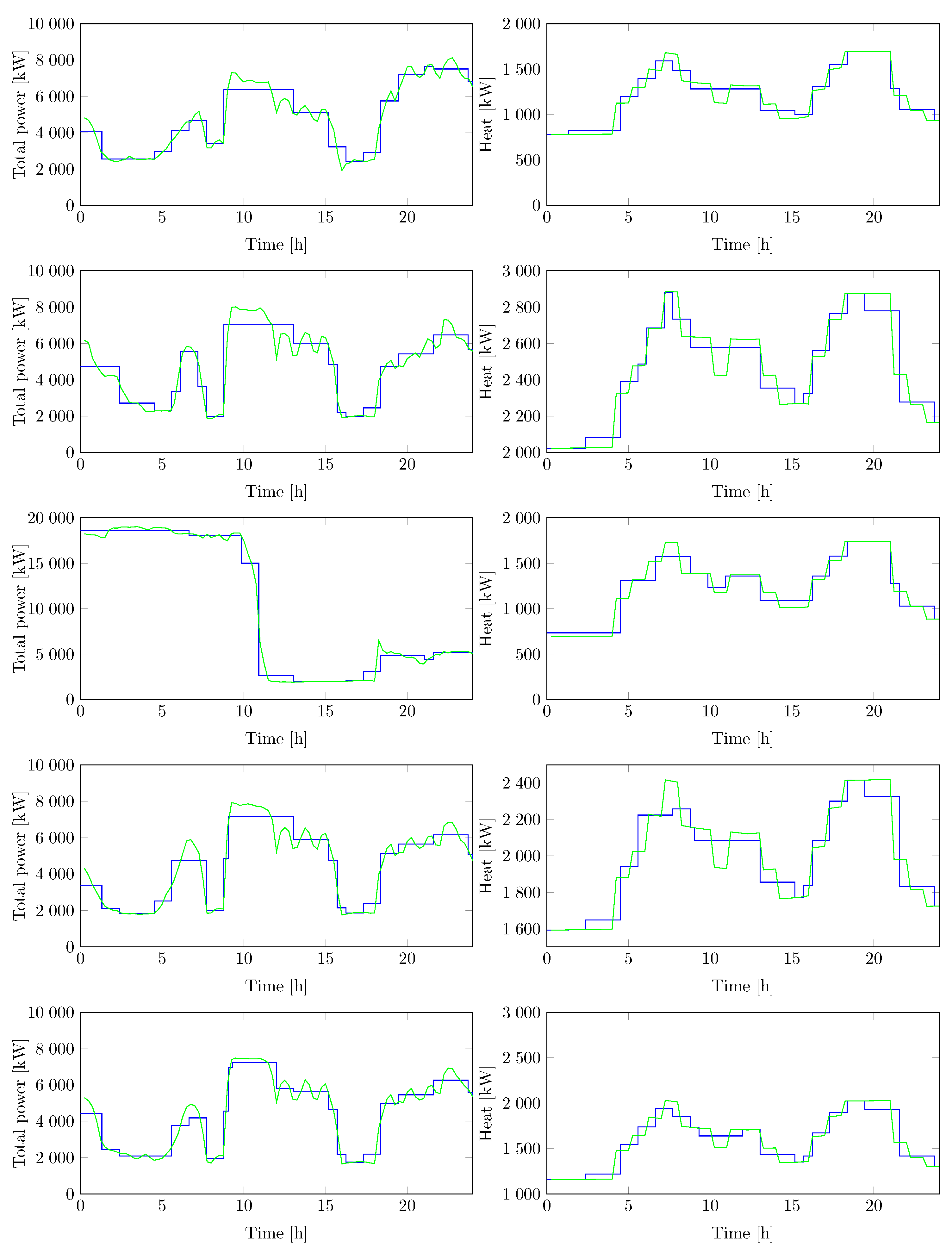
Figure 23.
Power (left) and exergy destruction (right) profiles, original (green) and segmented (blue), for the 2 typical days and duration curves.
Figure 23.
Power (left) and exergy destruction (right) profiles, original (green) and segmented (blue), for the 2 typical days and duration curves.

Table 1.
List of the main components of the ship energy systems.
| Unit Name | N | Rated Power | Other Info |
|---|---|---|---|
| Main engine | 4 | 5850 | 4-stroke, Nominal speed: 500 rpm, 6 cyl, Bore: 460 mm, Stroke: 580 mm, bsfc at rated power: 175 g/kWh |
| Auxiliary engine | 4 | 2760 | 4-stroke, Nominal speed: 750 rpm, 6 cyl, Bore: 320 mm, Stroke: 400 mm, bsfc at rated power: 184 g/kWh |
| HRSG (ME) | 2 | 800 | Based on 1000 kg/h steam at 7 bar. Only installed on ME2 and ME3 |
| HRSG (AE) | 4 | 640 | Based on 800 kg/h steam at 7 bar |
| Sea water cooler | 2 | 5400 | Based on a max water flow of 725 m/h |
| Electric generator | 4 | 3312 (kVA) | 8 poles, 50 Hz |
| Auxiliary boiler | 2 | 4500 | |
| HVAC–Preheater | 1 | 3500 | |
| HVAC–Reheater | 1 | 1780 | |
| HVAC–Compressors | 2 | 2015 |
Table 2.
Major contributors to ship exergy losses. Losses related to combustion are not included in the calculation.
Table 2.
Major contributors to ship exergy losses. Losses related to combustion are not included in the calculation.
| Component Name | Contribution to Exergy Losses |
|---|---|
| Turbochargers | 28.9% |
| HRSGs | 10.7% |
| Steam heater | 10.5% |
| HVAC preheater | 10.4% |
| Sea water cooler | 8.5% |
| Electric generators | 6.1% |
Table 3.
Performance parameters for the 5-cluster power and heat.
| 0.65 | 0.10 | |
| 0.11 | 0.11 | |
| 0.23 | 0.07 | |
| 0.18 | 0.06 | |
| 155.00 | 168.00 |
© 2018 by the authors. Licensee MDPI, Basel, Switzerland. This article is an open access article distributed under the terms and conditions of the Creative Commons Attribution (CC BY) license (http://creativecommons.org/licenses/by/4.0/).
Share and Cite
MDPI and ACS Style
Baldi, F.; Ahlgren, F.; Nguyen, T.-V.; Thern, M.; Andersson, K. Energy and Exergy Analysis of a Cruise Ship. Energies 2018, 11, 2508. https://doi.org/10.3390/en11102508
AMA Style
Baldi F, Ahlgren F, Nguyen T-V, Thern M, Andersson K. Energy and Exergy Analysis of a Cruise Ship. Energies. 2018; 11(10):2508. https://doi.org/10.3390/en11102508
Chicago/Turabian StyleBaldi, Francesco, Fredrik Ahlgren, Tuong-Van Nguyen, Marcus Thern, and Karin Andersson. 2018. "Energy and Exergy Analysis of a Cruise Ship" Energies 11, no. 10: 2508. https://doi.org/10.3390/en11102508
Note that from the first issue of 2016, this journal uses article numbers instead of page numbers. See further details here.