Optimal Dispatch of Microgrid with Combined Heat and Power System Considering Environmental Cost

Abstract

With the rapid development of wind power generation and photovoltaic power generation, the phenomenon of wind and solar abandoning becomes more and more serious in the operation of power systems, and the microgrid is a new operating mode of power systems which provides a new consumption mode for wind power generation. With the increasingly close connection among energy resources and people’s increasing awareness of environmental protection, this paper establishes a microgrid optimal scheduling model with a combined heat and power system, in consideration of environmental costs. This model aims at the lowest comprehensive cost, at the same time taking into account the emission reductions of SO₂ and NO_x, considering the cost of power generated by the micro-generator, environmental cost, the related cost of battery, operation and maintenance cost of wind power, and photovoltaic power generation. The related constraints of thermal balance and power balance are also considered during microgrid system operation. The established model is solved with an improved particle swarm algorithm. At last, taking a microgrid system as an example, the validity and reliability of the proposed model are verified.

1. Introduction

With the aggravation of environmental contamination and energy crisis, the bottleneck of traditional power generation is becoming more and more obvious. As a consequence, clean new energy generation forms are attracting more and more attention [1]. Wind power and photovoltaic power generation are the early forms of new energy generation, and the installed capacity and grid-connected scale have gradually increased. At the same time, its randomness and volatility pose great challenge to the safe operation of the power grid [2,3,4]. As a new form of network structure, microgrids can realize combined heat and power scheduling, give full play to the complementary characteristics of wind power generation and photovoltaic power generation [5], and realize local consumption of wind power and photovoltaic power generation, greatly reducing the amount of abandoned wind and photovoltaic energy. The problem of environmental pollution [6,7] is solved, to a certain extent.

With the deepening of relevant research, the advantages of microgrid economics, environmental protection, scheduling flexibility and other advantages, have gradually attracted the public’s attention [8,9,10], and field studies of microgrid systems are carried out in many areas. With the rise of the microgrid, how to determine the combined heat and power scheduling in the multisource microgrid system with wind and light storage [11,12], to achieve the goal of reducing the total operating costs and SO₂ and NO_x emissions, has become an urgent problem to be solved.

In recent years, the related research on microgrids has achieved certain results. In [13], Mao et al. comprehensively considered the operating cost, pollutant discharge, and operational risk, and established a multi-objective optimization model based on microgrids. It considered the impact of distributed power output volatility on microgrid operation, which can effectively improve the operation and management level of microgrids. In [14], Wu et al., based on the model of each power source in the microgrid, established the scheduling model when grid-connected, and proposed the mixed integer programming method applied to the optimal scheduling of the microgrid, which proves that this method has strong advantages in both computation time and calculation accuracy, and can provide fast and accurate scheduling information for short-term and ultra-short-term energy management of microgrids. In [15], Fubara et al. comprehensively considered the power balance and heat balance in a microgrid, and took the lowest operation cost as target, while considering the energy utilization rate, and two different operational strategies were proposed, which were applied to three different models. Through calculation, the operating costs under each power generation strategy were compared and verified. This contributed to the improvement of the energy efficiency of the microgrid. However, in [14,15], the investment of renewable energy, such as wind power and photovoltaics, is not taken into account, which can reduce the emission of pollutants to a certain degree. In [16], Thompson et al. established a multi-objective economic scheduling model with system operation cost, environmental benefit, and battery loss as evaluation indicators. An improved multi-objective particle swarm optimization (MOPSO) algorithm was proposed, which had better convergence and reduces the possibility of the algorithm falling into the local optimum. In [17] Lin et al. established an optimal scheduling model for hybrid power generation, in which renewable energy and batteries were considered. The enhanced bee colony optimization (EBCO) method was applied to solve the scheduling model. This method had better advantages in search efficiency and accuracy in high-dimensional space. The daily economic dispatch problem of the microgrid system could be better solved. In [18], Azizipanah-Abarghooee et al. constructed a microgrid scheduling model including micro-generators such as wind power, photovoltaic power generation, and combined heat and power units. The methods of chance-constrained and jointly distributed random variables are good proof that cogeneration scheduling has obvious economic benefits compared with single electrical scheduling. However, in [17,18], they did not consider the uncertainty of wind power forecasts nor the emission of pollutant. In [19], Lin et al. used the historical simulation method (HSM) to calculate the value at risk (VAR). Based on this, risk assessment of microgrid (MG) was conducted, and then according to the request of different confidence level, to develop a scheduling model of microgrid (MG). Finally, the reasonable balance between the risk and cost of microgrids was realized. In [20], Trivedi et al. proposed a whale optimization algorithm to solve the problem of combined economic emission dispatch (CEED), so as to minimize the total cost and total emissions of its microgrid operation. Compared with the gradient method (GM), ant colony optimization (ACO), and particle swarm optimizer (PSO) technique, separately, the optimal scheduling values obtained by whale optimization algorithm had more advantages in convergence speed and accuracy, which further proved the effectiveness and reliability of the algorithm. In [21], Tang et al. proposed a combined short-term load forecasting model based on empirical mode decomposition (EMD), extended Kalman filter (EKF), and extreme learning machine with kernel (KELM). The short-term load forecasting was carried out for the economic dispatch of microgrid to reduce the forecast error and ensure the system economic dispatch was optimal. The optimized particle swarm optimization algorithm [22,23,24] is used to solve some of the models mentioned in the literature above, which reduces the operating cost of the microgrid system.

In summary, in the operation of the microgrid, the best economic benefits can be obtained through reasonable scheduling. At present, the study of microgrid optimization scheduling, general, respectively, for the individual electric dispatch and electric heating joint scheduling [25,26,27], the former model is relatively simple, but in the study of combined thermoelectric scheduling, more attention is paid to economy, and the scheduling process taking environmental factors into account is rarely seen. With the enhancement of people’s awareness of environmental protection, the environmental factors in the operation of microgrids cannot be ignored.

This paper establishes a microgrid optimization scheduling model that takes into account the combined electric and thermal system under environmental costs, aiming at the lowest total cost and taking into account the emission reduction of SO₂ and NO_x. The power generation cost of micro-generators, environmental costs, the related cost of battery, operation and maintenance cost of wind power and photovoltaic power generation, are all considered in the total cost. The related constraints of thermal balance and power balance are also considered during microgrid system operation. This paper aims to reduce the operating cost of the system, and the emissions of SO₂ and NO_x. The impact of electricity price adjustment on microgrid scheduling cost is also analyzed. For wind power, photovoltaics, and other uncertain variables in the objective function, the clear equivalence forms are used to deal with this, so that the results are more accurate and realistic.

This paper is organized as follows: Section 2 and Section 3 establish the microgrid scheduling model, and give the respective target function and constraint conditions. Section 4 presents clear equivalence forms to deal with the uncertain variables in the model. Section 5 proposes an improved social particle swarm optimization algorithm to solve the microgrid scheduling model. Section 6 analyzes the results obtained by the microgrid model. Finally, Section 7 summarizes the conclusions.

2. Microgrid Objective Function Establishment

This article aims to minimize the comprehensive cost, at the same time taking into account the emission reductions of SO₂ and NO_x, based on the microgrid system with wind and solar storage, considering the cost of power generated by the micro-generator, environmental costs, operation and maintenance costs of wind power and photovoltaic power generation, and battery operating costs. In this paper, the microgrid structure is referred to [28] and improved on this basis, as shown in Figure 1, which consists of two thermal power generators (GEN), two combined heating and power units (CHP) containing heat storage devices, one wind turbine (WT), one unit of photovoltaic power generation equipment (PV), and one storage battery (SB) system. The combined heating and power unit includes two main parts: the microturbine (MT) and the bromine-cooling machine (BCM). The units in the network are uniformly controlled by the microgrid central controller (MGCC).

A scheduling model for a multisource microgrid power system was established. The objective function is as follows:

$$e=\min [e_1+e_2+e_3+e_4+e_5+e_6],$$

(1)

where e is the total operating cost of the microgrid system, e₁ is the cost of generating electricity for the micro-generator set; e₂ is the environmental cost; e₃ is the operation and maintenance cost of wind power generation; e₄ is the operation and maintenance cost of photovoltaic power generation; e₅ is the cost for exchanging energy between the microgrid system and the public power grid; e₆ is the operating cost of the battery.

2.1. Micro-Generator Set Generation Cost e₁

The micro-generator set includes two types of thermal power generators and combined heating and power units; both are coal-fired units. The cost of generating electricity for the micro-generator set includes the operating cost of thermal power generator and combined heating and power unit.

$$e_1=E_1(P_{it})+E_2(P_{ejt}),$$

(2)

where E₁ is the operating cost of the thermal power generator; E₂ is the operating cost of combined heating and power unit. P_it is the power output of the i-th thermal power generator during the t period, and P_ejt is the power output of the j-th combined heat and power unit during the t period.

A certain amount of fossil energy is consumed during the operation of thermal power generators, which will generate a certain cost of energy consumption. In the actual operation of thermal power generators, when the turbine intake valve suddenly opens, it will have a “valve point effect”, causing the generator’s consumption to increase, and the generator will have a certain start-up cost during the start-up process. Therefore, the calculation formula for the operating cost of a thermal power generator is as follows:

$$E_1={\displaystyle \sum _{t=1}^T{\displaystyle \sum _{i=1}^N\left\{\left[H(P_{it})+V(P_{it})+(1-S_{i(t-1)})B_{it}\right]S_{it}\right\}}},$$

(3)

$$H(P_{it})=a_i{P}_{it}{}^2+b_i{P}_{it}+c_i,$$

(4)

$$V(P_{it})=\left|e_i\sin \left[f_i(P_{it}-P_{imin})\right]\right|,$$

(5)

$$B_{it}={\gamma }_i+{\phi }_i(1-e^{-T_{it}^{off/{\theta }_i}}),$$

(6)

where H(P_it) is the energy cost of thermal power generator i in t period; a_i, b_i, c_i are the power generation cost coefficients of the thermal power generator i; V(P_it) is the energy consumption cost of the valve point effect of thermal power generator i during t period; e_i, f_i are the valve point effect coefficients of thermal power generator i; and P_imin is the lower limit of the output of thermal power generator i. S_it is the operating status of thermal power generator i during t period. S_it = 1 indicates unit operation, S_it = 0 indicates that the unit is out of service; B_it is the start-up cost of thermal power generator i during t period; γ_i, φ_i and θ_i are start-up cost factors for thermal power generator i; T_it^off is the downtime of thermal power generator i in t period. T is a scheduling period of the microgrid. In this paper, the scheduling period is divided into 24 periods, and N is the number of thermal power generators in the microgrid.

Combined heat and power unit as a heating unit cannot stop, therefore, the operating cost is the fuel cost. Equation (7) reference [29].

$$E_2={\displaystyle \sum _{t=1}^T{\displaystyle \sum _{j=1}^M\left\{a_{jr}{[P_{ejt}+c_v(P^r{}_{hit}+P^c{}_{hit,1}-P^c{}_{hit,2})]}^2+b_{jr}[P_{ejt}+c_v(P^r{}_{hit}+P^c{}_{hit,1}-P^c{}_{hit,2})]+c_{jr}\right\}}}$$

(7)

where P^r_hit is the total thermal power of the heat storage of the combined heat and power unit j during t period; P^c_hit,1 and P^c_hit,2 are the storage and release power of the heat storage device in the t period; a_jr, b_jr, c_jr are the fuel cost coefficients of the combined heat and power unit j respectively; c_v is the amount of change in electrical output when each unit heat output is increased for combined heat and power unit. M is the number of combined heat and power units in the microgrid.

2.2. Environmental Cost e₂

With the enhancement of the public’s environmental awareness, the requirements for the environmental protection of the power grid are increasing. The main contaminants considered in this paper are SO₂ and NO_x, and the environmental costs mainly include the operating costs of the desulfurization and denitrification devices and SO₂ and NO_x emission fees.

$$e_2=C_1+C_2,$$

(8)

where C₁ represents the operating cost of the desulfurization and denitrification device; and C₂ represents SO₂ and NO_x emission fees.

Among them, the calculation formulas for C₁ and C₂ are as follows:

$$C_1={\displaystyle \sum _{t=1}^T\left\{{\displaystyle \sum _{i=1}^N{P}_{it}}+{\displaystyle \sum _{j=1}^M[P_{ejt}+c_v(P^r{}_{hit}+P^c{}_{hit,1}-P^c{}_{hit,2})]+P_{tchange}}\right\}}(d_S{\eta }_S{C}_S+d_N{\eta }_N{C}_N),$$

(9)

$$\begin{array}{l}{C}_2={\displaystyle \sum _{t=1}^T({\displaystyle \sum _{i=1}^N{P}_{it}}+{\displaystyle \sum _{j=1}^M[P_{ejt}+c_v(P^r{}_{hit}+P^c{}_{hit,1}-P^c{}_{hit,2})]}}+P_{tchange})\\ (d_S(1-{\eta }_S)/L_S+d_N(1-{\eta }_N)/L_N)C_{NS}\end{array},$$

(10)

$$D=\left({\displaystyle \sum _{t=1}^T{\displaystyle \sum _{i=1}^N{P}_{it}+{\displaystyle \sum _{t=1}^T{\displaystyle \sum _{j=1}^M{P}_{ejt}}}}}\right)\left(d_S+d_N\right),$$

(11)

where d_S and d_N respectively generate the SO₂ and NO_x quality for the each unit power generation of the coal-fired unit; η_S and η_N are the efficiency of the desulfurization and denitrification devices respectively; C_S and C_N are the cost of removing SO₂ and NO_x per unit; L_S and L_N are the pollution equivalent values of SO₂ and NO_x respectively; and C_NS is the standard for the fee of SO₂ and NO_x for each amount of pollution. D is the total amount of pollutant emission of the generator set. P_tchange is the exchange power of the microgrid system with the public power grid during t period.

2.3. Operation and Maintenance Costs of Wind Power and Photovoltaic Power Generation e₃, e₄

Wind power generation and photovoltaic power generation are both new energy power generation forms, which do not generate environmental pollution during operation. They are clean energy and have strong competitiveness and broad prospects in future development. In this paper, the operation and maintenance costs of wind power and photovoltaic power generation are expressed as linear relations with their respective output power. The calculation formula is as follows:

$$e_3={\displaystyle \sum _{k=1}^K{\displaystyle \sum _{t=1}^T{C}_{wk}{P}_{wkt}}},$$

(12)

where C_wk is the operational maintenance cost coefficient for wind turbine k; P_wkt is the power generated by wind farm k during t period; and K is the number of wind turbines in the microgrid.

$$e_4={\displaystyle \sum _{l=1}^Q{\displaystyle \sum _{t=1}^T{C}_{vl}{P}_{vlt}}},$$

(13)

where C_vl is the operating and maintenance cost coefficient of the photovoltaic power station l; P_vlt is the power generated by photovoltaic power station l during t period. Q is the number of photovoltaic power stations in the microgrid.

2.4. The Cost of Exchanging Energy between the Microgrid System and the Public Power Grid e₅

The microgrid system is capable of power transmission with the public power grid, to ensure the microgrid system can operate safety. When the power provided by the power supply inside the microgrid system cannot meet the load demand, there is a need to buy electricity from the public grid. When the power generated by the internal power supply exceeds the load demand, excess power can be sold to the public power grid, therefore, it also plays the role of system rotary reserve. Equations (15) and (16) are from reference [10]. The cost for exchanging energy between the microgrid system and the public power grid is as follows:

$$e_5=C_{buy}+C_{sell,1},$$

(14)

where C_buy is the cost of the microgrid system to purchase electricity from the public grid; and C_sell,1 is the revenue from the sale of electric energy from the microgrid system to the public grid.

Among them, the calculation formulas of C_buy and C_sell,1 are as follows:

$$C_{buy}={\displaystyle \sum _{t=1}^T{P}_{tchange}{C}_{tgrid}}(P_{tchange}>0),$$

(15)

$$C_{sell,1}={\displaystyle \sum _{t=1}^T{P}_{tchange}{S}_{tgrid}}(P_{tchange}<0),$$

(16)

where P_tchange is the exchange power of the microgrid system with the public grid during t period; P_tchange > 0 indicates that the microgrid system purchases electricity from the public grid, and P_tchange < 0 indicates that the microgrid system sells electricity to the public grid; C_tgrid is the price of electricity for the public grid sells electricity to the microgrid during t period; and S_tgrid is the price of electricity when the microgrid sells electricity to the public grid during t period.

2.5. Storage Battery Operating Cost e₆

When the power generation of the internal power supply of the microgrid system is higher than the load demand, it can be sold to the public power grid, or excess electric energy can be stored in the storage battery as a system backup power supply. The storage battery will generate a certain cost during operation. In this paper, the operating cost of the storage battery is expressed as a positive correlation function between charge and discharge power and sold electric energy, as follows:

$$e_6={\displaystyle \sum _{t=1}^T{P}_{cha,ct}{C}_{cha}}+{\displaystyle \sum _{t=1}^T{P}_{dis,ct}{C}_{dis}}+{\displaystyle \sum _{t=1}^T{P}_{sell}}{C}_{sell,2},$$

(17)

where C_cha and C_dis are the operating cost of the storage battery unit charging and discharging power respectively; P_cha,ct, P_dis,ct are the charging and discharging power of the storage battery during t period. P_sell sells electricity to the public power grid for the storage battery during t period, and C_cell,2 is the electricity price when the storage battery is sold to the public power grid during t period.

3. Operational Constraints of Micro-Sources within the Microgrid

The microgrid has a complete power system structure and can interact with the public power grid at the same time, which further ensures the reliable operation of the microgrid system. In order to ensure the security of the microgrid system, it is necessary to satisfy relevant constraints, and the main constraints considered in this paper are as follows:

3.1. Thermal Power Generator Output Constraint

The output constraint for the thermal power generator is as follows:

$$P_{imin}\le P_{it}\le P_{imax},$$

(18)

where P_imin and P_imax are the lower and upper limits of the electric output of the thermal power generator i.

3.2. Thermal Power Generator Ramp Rate Constraint

The ramp rate constraint for the thermal power generator is as follows:

$$-r_{di}\le P_{it}-P_{i(t-1)}\le r_{ui},$$

(19)

where r_ui and r_di are the ramp-up rate constraint values and the ramp-down rate constraint values of the thermal power generator i.

3.3. Thermal Power Generator Output Constraint When Starting and Stopping

When the unit is out of service or from operation to downtime, the output of the unit should meet the minimum output:

$$\begin{array}{l}{S}_{i(t-1)}=0,S_i=1\\ S_i=1,S_{i(t+1)}=0\end{array}\}{P}_{it}=P_{imin}.$$

(20)

3.4. Combined Heat and Power Unit Electric Output Constraint

The electric output constraint for the combined heat and power unit is as follows:

$$P_{ejmin}\le P_{ejt}\le P_{ejmax},$$

(21)

where P_ejmin and P_ejmax are the lower and upper limits of the electric output of the combined heat and power unit j.

3.5. Combined Heat and Power Unit Thermal Output Constraint

The thermal output constraint for the combined heat and power unit is as follows:

$$0\le P^r{}_{hit,1}\le P^r{}_{hitmax},$$

(22)

where P^r_hit,1 is the thermal output of the combined heat and power unit j during t period; P^r_hitmax is the thermal output upper limit of the combined heat and power unit.

3.6. Combined Heat and Power Unit Ramp Rate Constraint

The ramp rate constraint for the combined heat and power unit is as follows:

$$-r^r{}_{dj}\le P_{ejt}-P_{ej(t-1)}\le r^r{}_{uj}$$

(23)

where r^r_uj and r^r_dj are the ramp-up rate constraint values and the ramp-down rate constraint values of the combined heat and power unit.

3.7. Storage Battery Charging Capacity Constraint

In order to ensure the service life of the battery and the battery can be used safely, the occurrence of overcharge and overdischarge of the battery shall be prevented, that is, it shall meet the constraints of certain upper and lower limits of capacity:

$$C_{min}\le C_t\le C_{max},$$

(24)

where C_max and C_min are the upper and lower limits of the battery state of charge; and C_t is the state of charge of the battery t.

The formula for C_t is as follows:

$$C_t=C_{t-1}+P_{cha,ct}-P_{dis,ct},$$

(25)

where P_cha,ct is the charging amount of the battery during the t period, and P_dis,ct is the discharging amount of the battery during the t period.

3.8. Storage Battery Charge and Discharge Power Constraint

Taking into account the battery charging and discharging power directly affect the battery’s service life and operating safety, therefore, the battery charging and discharging power need to meet the constraints of the certain limit, that is

$$\{\begin{array}{l}{P}_{dis,min}\le P_{dis,ct}\le P_{dis,max}\\ P_{cha,min}\le P_{cha,ct}\le P_{cha,max}\end{array},$$

(26)

where P_cha,max and P_dis,max are the upper limit of the charging and discharging power of the battery, and P_cha,min and P_dis,min are the lower limits of the charging and discharging power of the battery, respectively.

3.9. Charge and Discharge Constraint of the Battery at the Same Time

At the same time, the battery cannot charge and discharge at the same time, that is:

$$X_t·Y_t=0,$$

(27)

where X_t and Y_t are the battery’s charging and discharging states respectively, where X_t∈{0, 1}, Y_t∈{0, 1}.

3.10. Storage Battery Beginning and Ending Power Constraint

In order to meet the scheduling requirements of the next dispatch day and the safety operation of the battery, it is necessary to ensure that the battery’s electricity is equal to the initial battery’s electricity at the end of scheduling period, that is

$$C_{t0}=C_T,$$

(28)

where C_t0 and C_T are the initial value and the final value of the storage battery power during the scheduling period, respectively.

3.11. Heat Storage Device Capacity Constraint

The capacity constraint for the heat storage device is as follows:

$$C^r{}_{min}\le C^r{}_t\le C^r{}_{max},$$

(29)

where C^r_min and C^r_max are the minimum and maximum heat storage of the heat storage device; and C^r_t is the heat storage of the heat storage device during t period.

C^r_t is calculated as follows:

$$C^r{}_t=C^r{}_{t-1}+P^c{}_{hit,1}-P^c{}_{hit,2},$$

(30)

where P^c_hit,1 and P^c_hit,2 are the store and release power of the heat storage device during t period.

3.12. Heat Storage Device Beginning and Ending Heat Storage Constraint

The beginning and ending heat storage constraint for the heat storage device is as follows:

$$C^r{}_{t0}=C^r{}_T,$$

(31)

where C^r_t0 and C^r_T are the initial and final value of heat storage in the heat storage device scheduling period, respectively.

3.13. Heat Storage Device Storage and Exhaust Heat Constraint

The storage and exhaust heat constraint for the heat storage device is as follows:

$$P^c{}_{hit,1}{P}^c{}_{hit,2}=0$$

(32)

3.14. The Exchange Power of the Microgrid System with the Public Grid Constraint

The exchange power constraint for the microgrid system with the public grid is as follows:

$$P_{tchange,min}\le P_{tchange}\le P_{tchange,max},$$

(33)

where P_tchange,max and P_tchange,min are the upper and lower limits of the exchange power between the microgrid and the public power grid.

4. Processing of Uncertain Variables in Objective Function

4.1. System Credibility Opportunity Constraint

Wind power and photovoltaic power generation are fluctuating power supplies, have a certain degree of randomness, and the load and battery are also uncertain. Therefore, the wind power output, photovoltaic power output, battery output and load are represented by fuzzy parameters. That is, the power balance constraint is established at the confidence level α, which is

$$\mathrm{Cr}\left\{{\tilde{P}}_{lt}-{\displaystyle \sum _{i=1}^N{P}_{it}}-{\displaystyle \sum _{j=1}^M{P}_{ejt}}-{\displaystyle \sum _{k=1}^K{\tilde{P}}_{wkt}}-{\displaystyle \sum _{l=1}^Q{\tilde{P}}_{vlt}}-P_{tchange}-{\tilde{P}}_{cit}=0\right\}\ge \alpha ,$$

(34)

where P_lt is the demand for the load in the system during the period t. ${\tilde{P}}_{lt}$ is the fuzzy parameter of load demand; ${\tilde{P}}_{wkt}$, ${\tilde{P}}_{vlt}$ is the fuzzy parameter of the volatility power output of wind power and photovoltaic power generation; and P_cit is the power output of battery during t period, with P_cit > 0 indicating battery discharge, and P_cit < 0 indicating battery storage. ${\tilde{P}}_{cit}$ is the fuzzy parameter of the battery fluctuation output, Cr{·} is the credibility of the event in {·}, and α is the confidence level.

4.2. The Clear Equivalence Class of Fuzzy Chance Constraints

The fuzzy parameter ${\tilde{G}}_F$ of fluctuating power output and load in each scheduling can be represented by trapezoidal functions:

$$\mu (G_F)=\{\begin{array}{l}\frac{G_{F4}-G_F}{G_{F4}-G_{F3}},G_{F3}<G_F\le G_{F4}\\ 1,G_{F2}<G_F\le G_{F3}\\ \frac{G_F-G_{F1}}{G_{F2}-G_{F1}},G_{F1}<G_F\le G_{F2}\\ 0,others\end{array},$$

(35)

where μ(G_F) is a membership function; G_Fs (s = 1, 2, 3, 4) is a membership parameter; and G_Fs can be determined based on the predicted value G_fc.

G_F1–G_F4 can be determined based on the predicted value G_fc:

$$G_{Fs}={\omega }_s{G}_{fc},s=1,2,3,4;$$

(36)

where ω_s (s = 1, 2, 3, 4) is a proportional coefficient, 0 < ω_s < 1. The proportional coefficient is generally determined by the historical data of the fluctuating power output and load.

Trapezoidal fuzzy parameters can be represented by quadruplets:

$${\tilde{G}}_F=(G_{F1},G_{F2},G_{F3},G_{F4})=G_{fc}({\omega }_1,{\omega }_2,{\omega }_3,{\omega }_4),$$

(37)

Trapezoidal fuzzy parameters are shown in Figure 2.

The constraint function g(x, ξ) has the following form:

$$g(x,\xi )=h_1(x){\xi }_1+h_2(x){\xi }_2+\dots +h_t(x){\xi }_t+h_0(x),$$

(38)

where ξ_k is a trapezoidal fuzzy parameter (r_s1, r_s2, r_s3, r_s4), s = 1, 2, …, t, t∈R; and r_s1–r_s4 is a membership parameter.

The fuzzy parameter causes the constraint condition to not give a certain feasible set, so the confidence level is introduced, and it is hoped that the constraint condition is established with a certain confidence level α, expressed as

$$Cr\left\{g(x,\xi )\le 0\right\}\ge \alpha ,$$

(39)

where α is the confidence level; and Cr{·} is the credibility of the event in {·}.

Define two functions:

$$h_{\beta }^{+}(x)=\{\begin{array}{l}{h}_{\beta }(x),h_{\beta }(x)\ge 0\\ 0,h_{\beta }(x)<0\end{array},$$

(40)

$$h_{\beta }^{-}(x)=\{\begin{array}{l}0,h_{\beta }(x)\ge 0\\ -h_{\beta }(x),h_{\beta }(x)<0\end{array},$$

(41)

where β = 1, 2, …, t. Specially, if h(x) = 1, then h⁺(x) = 1, h⁻(x) = 0; if h(x) = −1, then h⁺(x) = 0, h⁻(x) = 1.

When the confidence level of the opportunity constraint is α ≧ 0.5, the clear equivalence form of the opportunity constraint (Equation (38)) is

$$\begin{array}{l}(2-2\alpha ){\displaystyle \sum _{s=1}^t[r_{s3}{h}_{\beta }^{+}(x)-r_{s2}{h}_{\beta }^{-}(x)]}+\\ (2\alpha -1){\displaystyle \sum _{s=1}^t[r_{s4}{h}_{\beta }^{+}(x)-r_{s1}{h}_{\beta }^{-}(x)]+}{h}_0(x)=0\end{array},$$

(42)

According to the above method, the fuzzy opportunity constraint is processed to obtain the clear equivalence form of the power balance constraint:

$$\begin{array}{l}(2-2\alpha )\left(P_{lt3}-{\displaystyle \sum _{k=1}^K{P}_{wkt2}}-{\displaystyle \sum _{l=1}^Q{P}_{vlt2}}-P_{\mathrm{c}it2}\right)+(2\alpha -1)\left(P_{lt4}-{\displaystyle \sum _{k=1}^K{P}_{wkt1}}-{\displaystyle \sum _{l=1}^Q{P}_{vlt1}}-P_{\mathrm{c}it1}\right)\\ -{\displaystyle \sum _{i=1}^N{P}_{it}}-{\displaystyle \sum _{j=1}^M{P}_{ejt}}-P_{tchange}=0\end{array}.$$

(43)

5. Improved Social Particle Swarm Optimization

5.1. Social Particle Swarm Optimization

The social particle swarm optimization algorithm sets have different audience thresholds for each individual and, accordingly, determine whether the individual follows other individuals or maintains the current state, or is free to move. In order to maintain the diversity of individuals in the population, avoid premature convergence of the algorithm and fall into a local optimum.

There are two types of particles in the social particle swarm algorithm: free particles and following particles. The free particle is a particle with a threshold value of 0. It is not affected by the behavior of other particles, and randomly determines the position of the next generation of particles. Particles with non-zero thresholds are followed by particles which are affected by the attraction point during the search process. Whether or not they follow the attraction point depends on how many other follower particles are present. The SPSO algorithm follows the particle update formula as:

$$v_{ij}\left(t+1\right)=\omega v_{ij}\left(t\right)+c_1{r}_1\left(pbes{t}_{ij}\left(t\right)-x_{ij}\left(t\right)\right)+c_2{r}_2\left(attrac{t}_{ij}\left(t\right)-x_{ij}\left(t\right)\right),$$

(44)

$$x_{ij}\left(t+1\right)=x_{ij}\left(t\right)+v_{ij}\left(t+1\right),$$

(45)

where ω is the inertia weight, indicating the impact of the historical velocity information of the particle on the current velocity; c₁ and c₂ are learning factors; and r₁ and r₂ are random numbers of [0,1].

Among them, the third term in the above formula is changed from the gbest_ij in the standard PSO to the attraction point attract_ij, which may also be different for different particles. When the algorithm is initialized, the following particle selects the individual with the best fitness value of the population as the initial attraction point, and the algorithm is consistent with the standard PSO algorithm. As the search progresses, each free particle may become a new attraction point. If the fitness value of a certain free particle k is better than the fitness value of all other particles, then k becomes the attraction point. At this time, individuals with a threshold value of 1 in the following particle will be attracted first, and then individuals with a higher threshold value will also move toward the attraction point. Individuals whose number of attracted populations do not reach the threshold will maintain the original searching mode.

5.2. Improvement of Weight ω

It is proposed that the inertia weight of each particle decreases not only with the increase of the number of iterations, but also decreases as the distance from the global best point increases. That is, the inertia weight ω dynamically changes according to the position of the particle:

$$\omega \left(t\right)={\omega }_{start}-\frac{\left(l_{xg}-l_{min}\right)\left({\omega }_{start}-{\omega }_{end}\right)t}{\left(l_{max}-l_{min}\right)t_{max}},$$

(46)

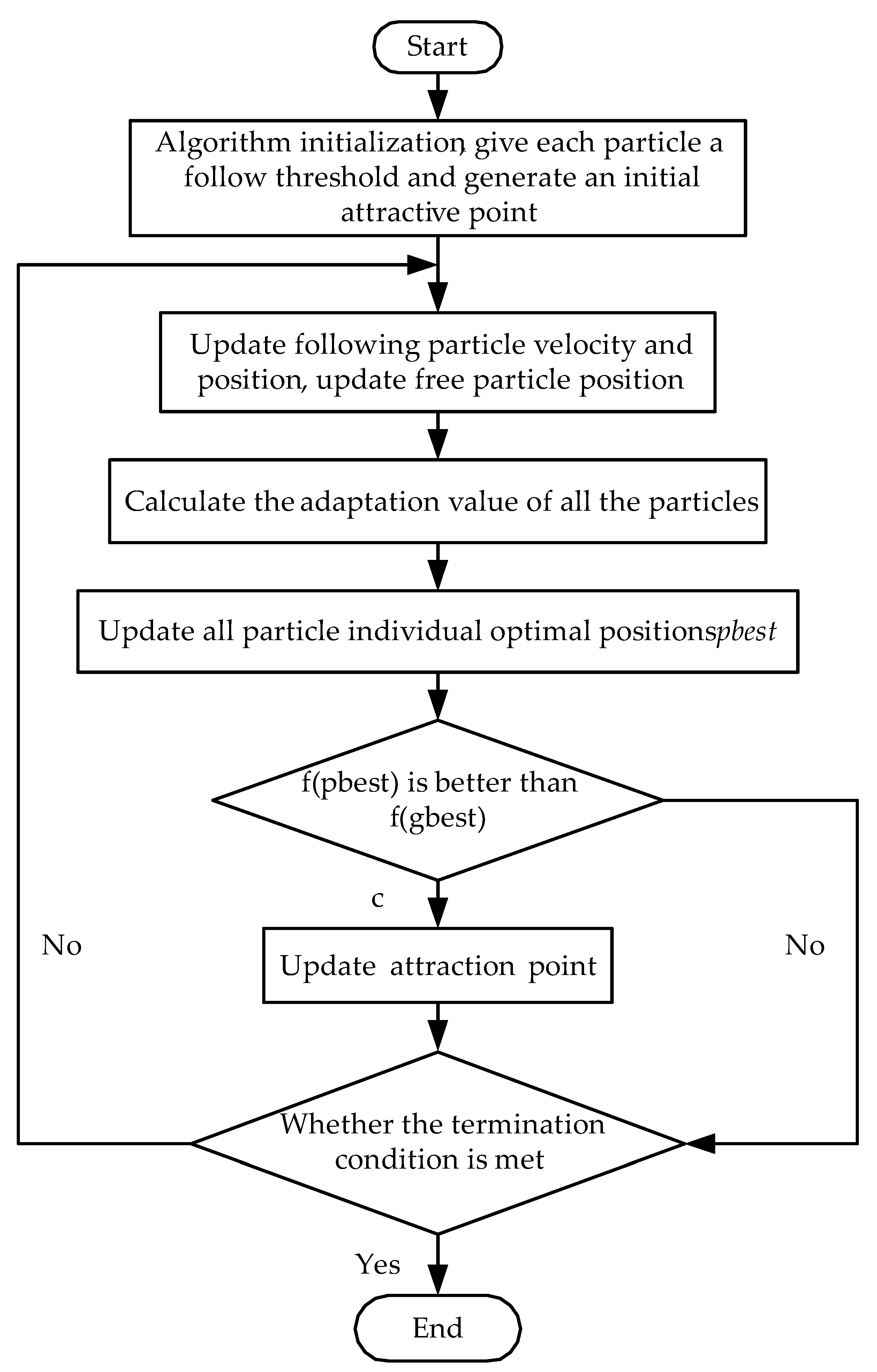
where l_xg is the distance from the particle x to the optimal particle, and l_max and l_min are the preset parameters of maximum distance and minimum distance, respectively. According to the above formula, when l_xg > l_max, ω = ω_start; when l_xg < l_min, ω = ω_end; when l_min < l_xg < l_max, ω increases monotonically with l_xg. Simulation results show that the algorithm has a significant improvement in convergence speed and convergence accuracy under this strategy. The flowchart for improved standard particle swarm optimization (SPSO) is shown in Figure 3.

6. Example Analysis

6.1. System Example Summarize

The microgrid system consists of two thermal power generators, two combined heating and power units with thermal storage units, one wind turbine unit, one photovoltaic power generation unit, and one battery system. The relevant data of wind power and photovoltaic power generation in the microgrid are shown in

Table 1. Distributed power parameters of microgrid.

Generator Type	Minimum Power/MW	Maximum Power/MW	Operation and Maintenance Costs/($/MW∙h)
(PV)	0	0.104	17.467
(WT)	0.002	0.246	14.556
(SB)	0	2.000	29.112

, which references [10], and the relevant parameters of the thermal power generator are shown in

Table 2. Conventional thermal power generator parameters.

Thermal Power Generator	Pimax/MW	Pimax/MW	Rui/(MW/h)	Rdi/(MW/h)	Power Generation Cost Coefficient
					a1 ($/MW2)	a2 ($/MW)	a3 ($)
Unit 1	2	1	0.500	0.500	1.746 × 10−4	2.929	20.713
Unit 2	2	0.800	1	1	7.424 × 10−3	8.798	44.047

. Coefficients of combined heating and power units are shown in

Table 3. Combined heat and power unit parameters.

Unit Type	Pejmax/MW	Pejmin/MW	Rrui/(MW/h)	Rrdi/(MW/h)	Prhitmax/MW
						CHP	3	1	1	1	3

and

Table 4. Combined heat and power unit parameters.

Unit Type	Cogeneration Unit Fuel Cost Coefficient
	ajr ($/MW2)	bjr ($/MW)	cjr ($)	cv
CHP	7.86 × 10−3	23.354	128.035	0.150

, and related data of batteries are shown in Table 1,

Table 5. Data of storage battery.

The Unit Type	Cn/MW∙h	Cmax/MW∙h	Cmin/MW∙h	Ct0/MW∙h	CT/MW∙h
(SB)	5	4.750	1.750	2	2

, and

Table 6. Data of storage battery.

The Unit Type	Tn/times	Ccha/($/MW∙h)	Cdis/($/MW∙h)	Csell/($/MW∙h)
(SB)	8	0.015	0.015	0.022

. Pollutant emissions of each unit are shown in

Table 7. Correlation coefficient of environmental cost calculation.

Correlation Coefficient of Environmental Cost Calculation
dS/kg	dN/kg	ηS/%	ηN/%	CS ($/kg∙MW∙h)	CN ($/kg∙MW∙h)	LS/kg	LN/kg	CNS/$
0.206	9.890	0.850	0.850	0.435	2.183	0.950	0.950	0.175

and

Table 8. Pollutant discharge coefficient of microgrid.

Contaminant Type	Pollutant Emission Coefficient/(kg/(MW·h))
	Coal-Fired Unit	PV	WT	SB	Ptchange
SO2	0.206	0	0	0	0.206
NOx	9.890	0	0	0	9.890

. Related parameters of heat storage device are shown in

Table 9. Related parameters of heat storage device.

Unit Type	Crmax/MW·h	Crmin/MW·h	Crt0/MW·h	CrT/MW·h
Heat storage device	4.750	1.750	2	2

. The exchange prices of microgrid and public power grid at each time period are shown in

Table 10. Electricity exchange price of microgrid and the public grid.

Time Period	0:00–7:00	7:00–10:00	10:00–15:00	15:00–18:00	18:00–21:00	21:00–00:00
Ctgrid ($/MW∙h)	32.023	61.135	94.614	61.135	94.614	61.135
Stgrid ($/MW∙h)	36.390	77.147	119.360	77.147	119.360	77.147

, which references [30]. This article selects a typical dispatch day as a research object and divides one day into 24 scheduling periods of one hour each. The forecast curve of load, wind power, and photovoltaic power generation is shown in Figure 4. The upper and lower limits of the exchange power between the microgrid and the public power grid are 2 MW and −2 MW, respectively (the microgrid absorbs power from the public power grid positively, otherwise it is negative). The number of charge and discharge times T_n of the battery is 8 times, and the rated capacity C_n is 5 MW∙h.

6.2. Example Result

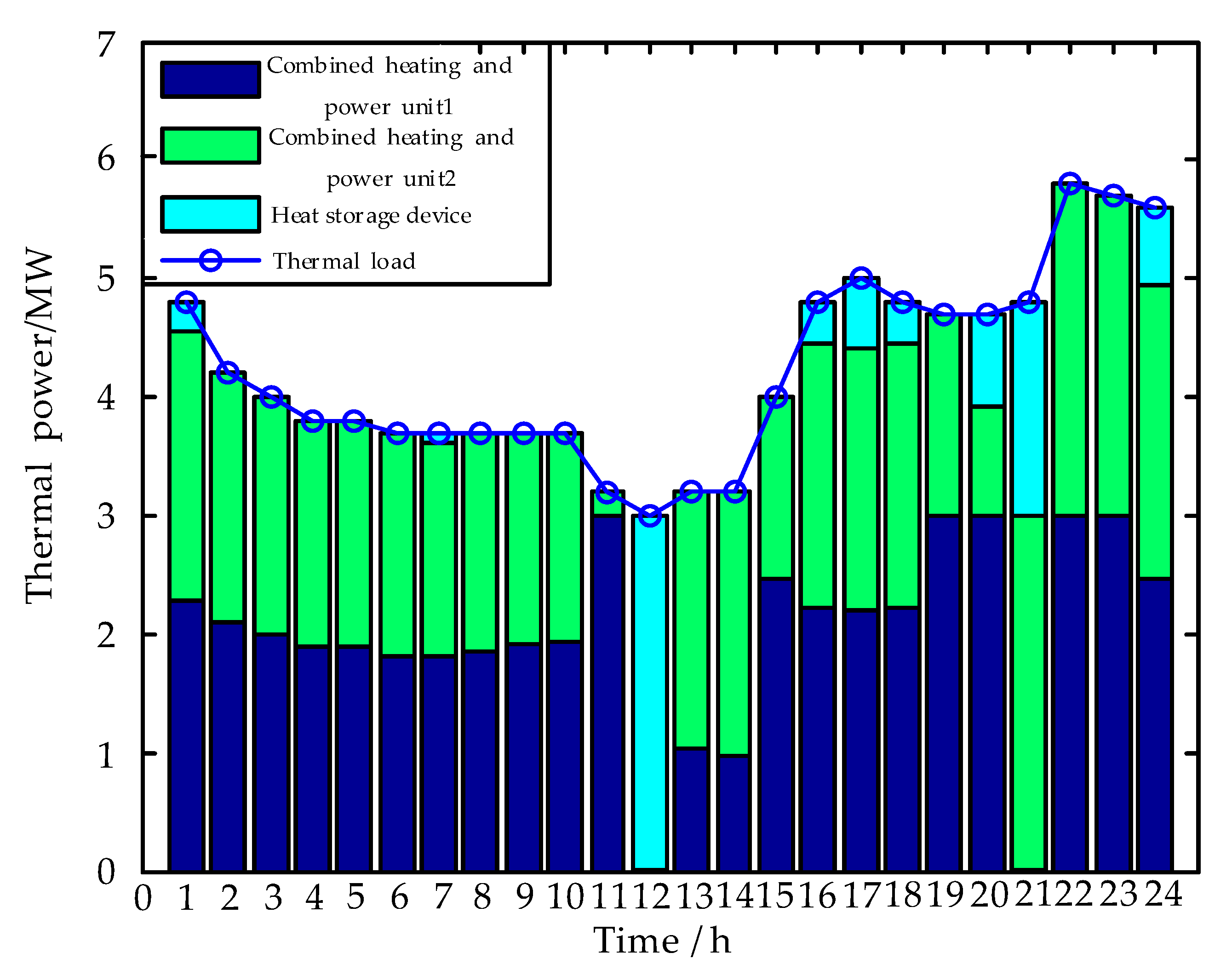
This paper has established a comprehensive consideration of the cost of power generation for micro-generator sets, environmental costs, operation and maintenance costs of wind power and photovoltaic power generation, and operating costs of batteries. A microgrid optimization scheduling model was built that included the combined heat and power system in consideration of environmental costs. Through the improved particle swarm algorithm, the minimum operating cost for the scheduled intraday microgrid system is 12,285 dollars. At this time, the scheduling curves of the power output of each micro-source are shown in Figure 5, and the thermal output of the combined heat and power units is shown in Figure 6.

Figure 5 shows the dispatch value of power generation output of each micro-generator when the total cost is the lowest. Both wind power and photovoltaic power generation are completely consumed in this dispatching process, that is, the maximum power follows the control. As can be seen from Figure 5, the thermal power generator and the combined heating and power unit serve as controllable units to track the change trend of the load to some extent.

As can be seen from Figure 6, the sum of the heat output of the combined heat and power unit and the heat storage device is equal to the value of the heat load, which satisfies the heat balance constraint during the operation. The heat storage device breaks the thermoelectric coupling characteristics of the combined heat and power unit, and realizes a reasonable dispatch of the unit’s heat output.

The battery storage capacity and charge or discharge power of the battery during this economic dispatch are shown in Figure 7.

As can be seen from Figure 7, for the storage battery, charging and discharging cannot be performed at the same time, and the charging and discharging amount of the storage battery are equal in a scheduling period. Compared with Figure 4, we can see that in the low-load period, the battery is charging. In the peak load period, the battery is discharging, which not only increased the peak capacity of the microgrid system, but also provides a new way for the consumption of new energy generation.

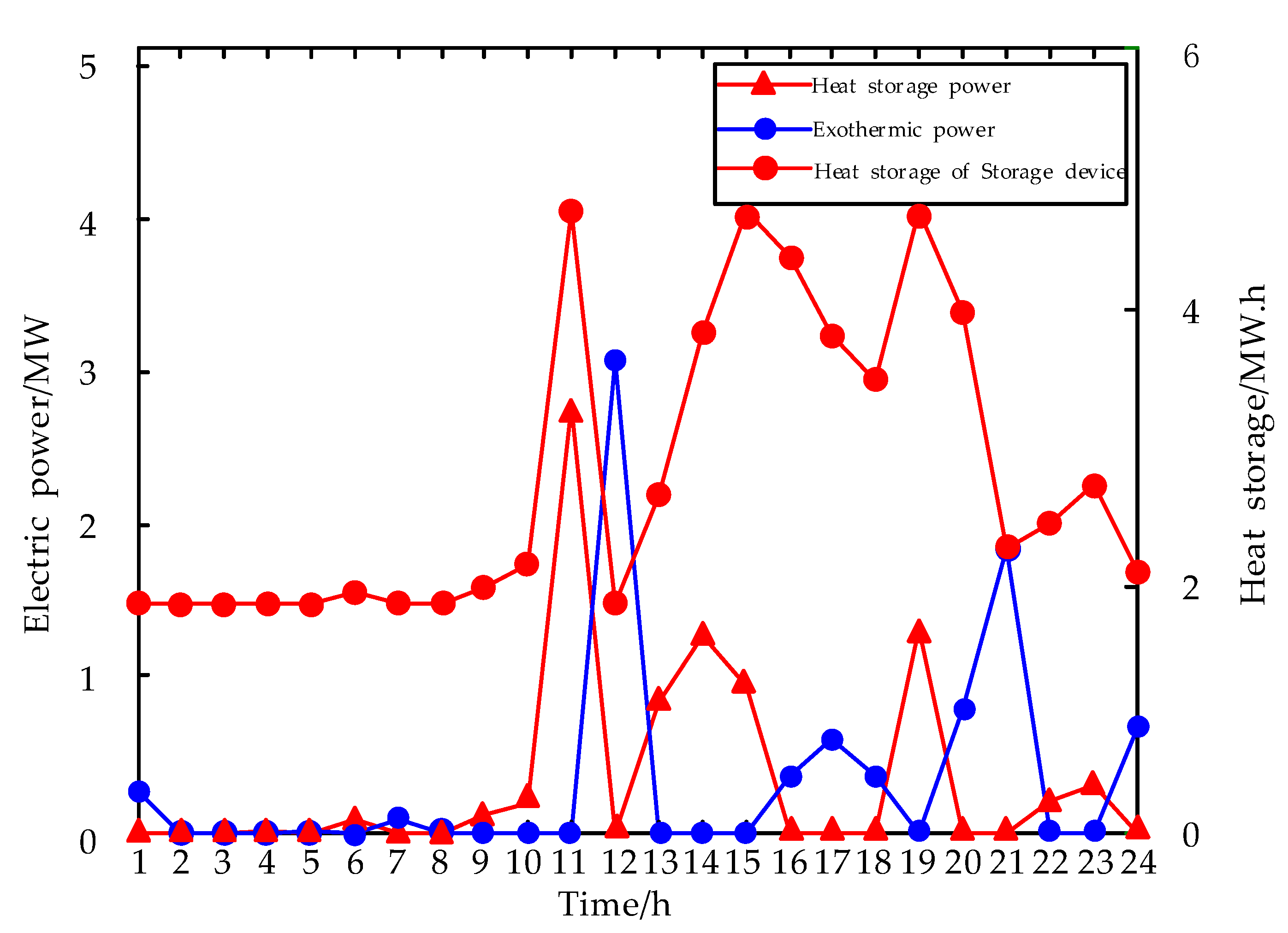
From Figure 8, it can be seen that the heat storage device cannot store and release heat at the same time, and the thermal storage capacity is the same as the thermal release capacity. After a scheduling period, the thermal storage remains unchanged, which ensures the normal operation of the next scheduling cycle.

6.3. Different Model Results

In order to verify the superiority of this paper’s scheduling model in consideration of environmental costs, it is compared with the conventional micro-network scheduling model that does not consider environmental costs, and is defined as follows.

Model 1: This article takes into account the environmental costs of the microgrid thermal-electric joint scheduling model.

Model 2: Traditional microgrid thermal-electric joint scheduling model without environmental costs.

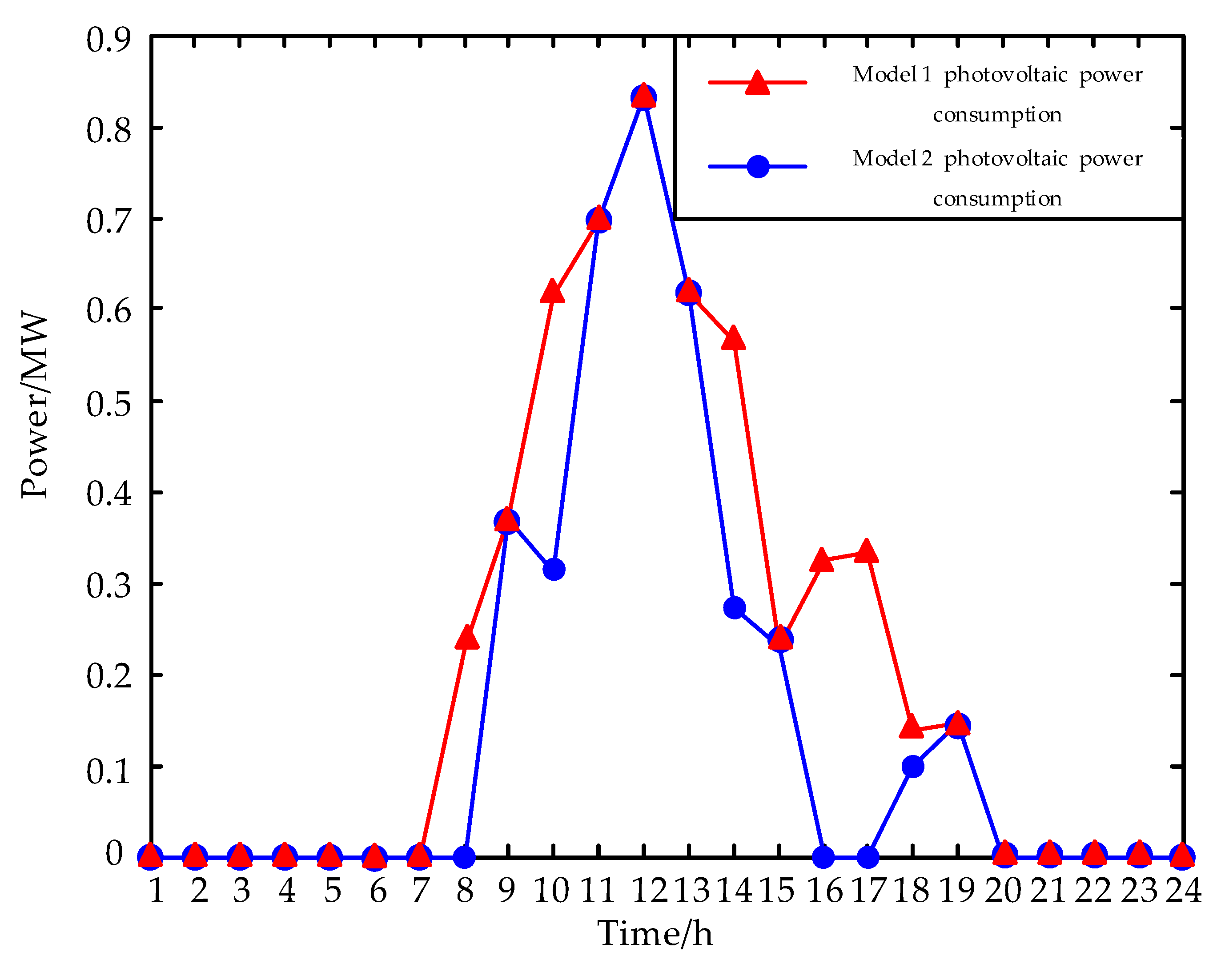
The comparison of wind power’s consumption under different scheduling models is shown in Figure 9, and the comparison of photovoltaic power consumption is shown in Figure 10.

From Figure 9 and Figure 10, it can be seen that for the consumption of wind power and photovoltaic power generation, model 1 is generally higher than model 2, that is, it can effectively increase the consumption of wind power generation after taking into account environmental costs, and promote the development of wind power generation.

The scheduling results for different models are shown in

Table 11. Scheduling results comparison of two models.

Model	Total Costs/$	Wind Power Consumption/%	Photovoltaic Consumption/%	SO2 Emissions/ton	NOx Emissions/ton
Model 1	12285	100	100	0.005	0.255
Model 2	8690	54.470	70.090	0.038	1.810

.

From Table 11, it can be seen that in terms of comprehensive cost, model 1 is increased by 3595 dollars compared with model 2. However, in terms of wind power generation’s consumption, model 1 achieved complete absorption of wind power generation and photovoltaic power generation, and the wind power’s consumption increased by 45.53% compared with model 2, and the photovoltaic power generation’s consumption increased by 29.91% compared with model 2. Regarding the emission of pollutants, model 1 reduced SO₂ and NO₂ emissions by 0.033 tons and 1.555 tons, respectively, compared with model 2, which can significantly promote the development of electricity and environmental protection.

Taking into account that the environmental costs in the scheduling process can significantly increase the amount of wind power generation and photovoltaic power generation, and reduce SO₂ and NO_x emissions, for new energy generation and environmental protection, this development has great significance.

6.4. Different Algorithm Results

In order to verify the superiority of the improved particle swarm optimization algorithm in terms of iterative speed and accuracy, the results obtained by the two algorithms are compared. The curve is shown in the following figure. Figure 11 and Figure 12 show the change curve of the scheduling cost and the amount of pollutant emissions with the number of iterations, obtained by the standard particle swarm optimization algorithm. Figure 13 and Figure 14 show the change curve of the scheduling cost and the amount of pollutant emissions with the number of iterations, obtained by the improved social particle swarm optimization algorithm.

Table 12. Comparison of two algorithm scheduling results.

Comparison of Results	SPSO	Improved SPSO
Scheduling cost e/k$	12.838	12.285
Pollutant emissions D/ton	0.370	0.260

shows the value of the scheduling cost and the amount of the pollutant emission finally obtained by the two algorithms.

It can be seen from the above figure that with the increase of the number of iterations, the scheduling cost and the amount of pollutant emissions obtained by the improved particle swarm optimization algorithm finally converge to the lowest value, which verifies the effectiveness of the algorithm. It can be seen from Figure 11 and Figure 12 that when the standard particle swarm optimization algorithm is used, the cost of the scheduling and the amount of pollutant emissions converge to the lowest value after 500 iterations. Figure 13 and Figure 14 show that the convergence speed is significantly improved after using the improved particle swarm algorithm, and the lowest value is obtained after 300 iterations. In Table 12, the scheduling cost and the amount of pollutant emissions obtained by the improved particle swarm optimization algorithm are, respectively, 12,285 dollars and 0.26 tons. Compared with the results obtained by the standard particle swarm optimization algorithm, the superiority of the improved particle swarm optimization algorithm in convergence speed and accuracy is well verified.

6.5. The Effect of Adjustment of Time-of-Use Electricity Price on Scheduling Results

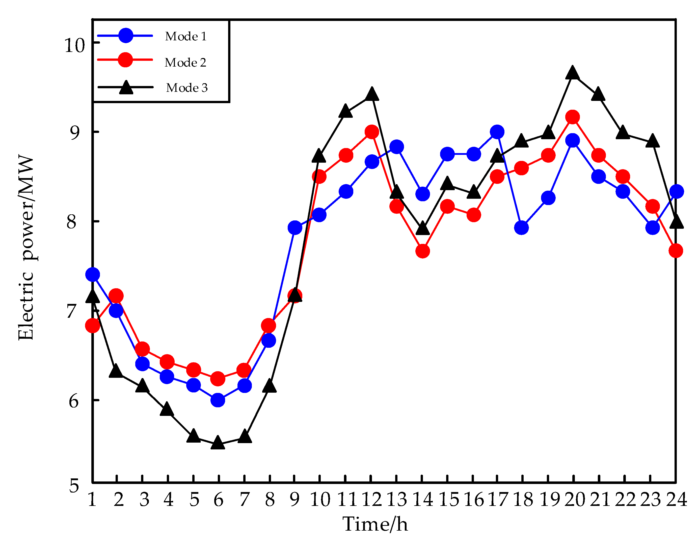
For the calculation of e₅ in the objective function, the time-of-use price is taken into account, and now adjusting the time-of-use price, to analyze the impact of price changes on microgrid scheduling. The electricity price is uniformly increased by 10% and reduced by 10%, respectively. The power generation output scheduling curve obtained is shown in the Figure 15.

From this, it can be seen that mode 1 is the power generation output curve obtained after increasing by 10%, and it can be seen that the peak valley difference is the smallest. Mode 2 is the power generation output curve under the original electricity price. Mode 3 is the curve obtained after 10% reduction, with the maximum peak valley difference. This is because after mode 1 increases the electricity price, restraining the demand of the load and shortening the peak valley difference becomes inevitable. After the electricity price is decreased in mode 3, the electricity consumption of users during peak hours will be increased, further increasing the peak valley difference.

For further increase or decrease of electricity price, the corresponding scheduling cost is shown in

Table 13. Scheduling cost under different electricity price.

Comparison of Results	Electricity Price Raised by 10%	Electricity Price Raised by 20%	The Original Price	Electricity Price Fell by 10%	Electricity Price Fell by 20%
Scheduling cost e/$	12,490	12,239	12,285	12,310	12,530

.

It can be seen from the table that after the electricity price increases by 10%, the scheduling cost is slightly reduced, but it is not obvious. After the electricity price 10% reduction, the scheduling cost increased slightly. When the electricity price is increased or decreased by 20%, the scheduling cost increases obviously. This is because when electricity prices are raised, load demand is suppressed, and peak valley difference reduced, thereby reducing the number of power generator start and stop times, saving the start-up cost and total cost of scheduling. When the electricity price is decreased, the demand of load during peak hours will be increased, increasing peak valley difference. The number of power generator start and stop times will be increased, so the scheduling costs will also increase. The results from the table show that the price of electricity cannot increase arbitrarily, and the scheduling cost will have a significant increasing due to the unreasonable electricity prices. Under the calculation parameters of this paper, for the adjustment of electricity price, it is reasonable to increase within 10 percentage points, if necessary.

7. Conclusions

This paper aims to minimize the total cost, while taking into account the emission reductions of SO₂ and NO_x, considering the power generation costs, the environmental costs of micro-generator sets, the operation and maintenance costs of wind power and photovoltaic power generation, the related cost of battery, and the operation and maintenance cost of wind power and photovoltaic power generation. The related constraints of thermal balance and power balance also considered during microgrid system operation. A microgrid optimization scheduling model was established that included a combined heat and power system in consideration of environmental costs. Taking a microgrid system as an example, the improved particle swarm optimization algorithm is used to verify the validity and reliability of the model, and it also proves the effectiveness and superiority of the improved algorithm. The impact of electricity price’s adjustment on microgrid scheduling cost also analyzed. The results show that, in this paper, the environmental cost scheduling model is compared with the traditional non-environmental cost scheduling model. Although the total cost has increased by 3595 dollars, the wind power consumption has increased by 45.53%, and the photovoltaic generation consumption has increased by 29.91%. SO₂ and NO_x emissions are respectively reduced by 0.033 tons and 1.555 tons, which has great significance for energy conservation and emission reduction.

References

- Arriagada, E.; López, E.; López, M.; Blasco-Gimenez, R.; Roa, C.; Poloujadoff, M. A probabilistic economic dispatch model and methodology considering renewable energy, demand and generator uncertainties. Electr. Power Syst. Res. 2015, 121, 325–332. [Google Scholar] [CrossRef]
- Zhang, Z.-S.; Sun, Y.-Z.; Gao, D.W.; Lin, J.; Chen, L. A versatile probability distribution model for wind power forecast errors and its application in economic dispatch. IEEE Trans. Power Syst. 2013, 28, 3114–3125. [Google Scholar] [CrossRef]
- Ren, B.; Jiang, C. A review on the economic dispatch and risk management considering wind power in the power market. Renew. Sustain. Energy Rev. 2009, 13, 2169–2174. [Google Scholar]
- Eftekharnejad, S.; Heydt, G.T.; Vittal, V. Optimal generation dispatch with high penetration of photovoltaic generation. IEEE Trans. Sustain. Energy 2015, 6, 1013–1020. [Google Scholar] [CrossRef]
- Xu, Q.; Ding, Y.; Zheng, A. An optimal dispatch model of wind-integrated power system considering demand response and reliability. Sustainability 2017, 9, 758. [Google Scholar] [CrossRef]
- Gjengedal, T.; Johansen, S.; Hansen, O. A qualitative approach to economic-environment dispatch-treatment of multiple pollutants. IEEE Trans. Energy Convers. 2002, 7, 367–373. [Google Scholar] [CrossRef]
- Zhong, J.-Q. Research on environmental economic dispatch of power system including wind farm. Phys. Procedia 2012, 24, 107–113. [Google Scholar]
- Moghaddam, A.A.; Seifi, A.; Niknam, T.; Pahlavani, M.R.A. Multi-objective operation management of a renewable MG (micro-grid) with back-up micro-turbine/fuel cell/battery hybrid power source. Energy 2011, 36, 6490–6507. [Google Scholar] [CrossRef]
- Motevasel, M.; Seifi, A.R.; Niknam, T. Multi-objective energy management of CHP (combined heat and power)-based micro-grid. Energy 2013, 51, 123–136. [Google Scholar] [CrossRef]
- Li, C.; Zhang, J.; Li, P. Multi-objective optimization model of micro-grid operation considering cost, pollution discharge and risk. Proc. CSEE 2015, 35, 1051–1058. [Google Scholar]
- Khorramdel, B.; Raoofat, M. Optimal stochastic reactive power scheduling in a microgrid considering voltage droop scheme of DGs and uncertainty of wind farms. Energy 2012, 45, 994–1006. [Google Scholar] [CrossRef]
- Fang, X.; Ma, S.; Yang, Q.; Zhang, J. Cooperative energy dispatch for multiple autonomous microgrids with distributed renewable sources and storages. Energy 2016, 99, 48–57. [Google Scholar] [CrossRef]
- Mao, M.; Ji, M.; Wei, D.; Chang, L. Multi-objective economic dispatch model for a microgrid considering reliability. In Proceedings of the 2nd International Symposium on Power Electronics for Distributed Generation Systems, Hefei, China, 16–18 June 2010. [Google Scholar]
- Wu, X.; Wang, X.; Wang, J.; Bie, Z. Economic generation scheduling of a microgrid using mixed integer programming. Proc. CSEE 2013, 33, 1–8. [Google Scholar]
- Fubara, T.C.; Cecelja, F.; Yang, A. Modelling and selection of micro-CHP systems for domestic energy supply: The dimension of network-wide primary energy consumption. Appl. Energy 2014, 114, 327–334. [Google Scholar] [CrossRef]
- Thompson, C.C.; Oikonomou, K.; Etemadi, A.H.; Sorger, V.J. Optimization of data center battery storage investments for microgrid cost savings, emissions reduction, and reliability enhancement. IEEE Trans. Ind. Appl. 2016, 52, 2053–2060. [Google Scholar] [CrossRef]
- Lin, W.-M.; Tu, C.-S.; Tsai, M.-T. Energy management strategy for microgrids by using enhanced bee colony optimization. Energies 2015, 9, 5. [Google Scholar] [CrossRef]
- Azizipanah-Abarghooee, R.; Niknam, T.; Bina, M.A.; Zare, M. Coordination of combined heat and power-thermal-wind-photovoltaic units in economic load dispatch using chance-constrained and jointly distributed random variables methods. Energy 2014, 79, 50–67. [Google Scholar] [CrossRef]
- Lin, W.-M.; Tu, C.-S.; Tsai, M.-T. An optimal scheduling dispatch of a microgrid under risk assessment. Energies 2018, 11, 1423. [Google Scholar] [CrossRef]
- Trivedi, I.N.; Bhoye, M.; Bhesdadiya, R.H.; Jangir, P.; Jangir, N.; Kumar, A. An emission constraint environment dispatch problem solution with microgrid using Whale Optimization Algorithm. In Proceedings of the 2016 National Power Systems Conference (NPSC), Bhubaneswar, India, 19–21 December 2016. [Google Scholar]
- Tang, Q.; Zhang, J.; Xie, Z. Short-term micro-grid load forecast method based on EMD-KELM-EKF. In Proceedings of the 2014 International Conference on Intelligent Green Building and Smart Grid (IGBSG), Taipei, Taiwan, 23–25 April 2014. [Google Scholar]
- Wang, L.; Singh, C. Environmental/economic power dispatch using a fuzzified multi-objective particle swarm optimization algorithm. Electr. Power Syst. Res. 2007, 77, 1654–1664. [Google Scholar] [CrossRef]
- Niknam, T.; Mojarrad, H.D.; Nayeripour, M. A new fuzzy adaptive particle swarm optimization for non-smooth economic dispatch. Energy 2010, 35, 1764–1778. [Google Scholar] [CrossRef]
- Mohammadi-Ivatloo, B.; Moradi-Dalvand, M.; Rabiee, A. Combined heat and power economic dispatch problem solution using particle swarm optimization with time varying acceleration coefficients. Electr. Power Syst. Res. 2013, 95, 9–18. [Google Scholar] [CrossRef]
- Gambino, G.; Verrilli, F.; Meola, D.; Himanka, M.; Palmieri, G.; Vecchio, C.D.; Glielmo, L. Model predictive control for optimization of combined heat and electric power microgrid. IFAC Proc. Vol. 2014, 47, 2201–2206. [Google Scholar] [CrossRef]
- Sun, T.; Lu, J.; Li, Z.; Lubkeman, D.L.; Lu, N. Modeling combined heat and power systems for microgrid applications. IEEE Trans. Smart Grid 2017, 9, 4172–4180. [Google Scholar] [CrossRef]
- Zidan, A.; Gabbar, H.A.; Eldessouky, A. Optimal planning of combined heat and power systems within microgrids. Energy 2015, 93, 235–244. [Google Scholar] [CrossRef]
- Li, Z.; Zhang, F.; Liang, J.; Yun, Z.; Zhang, J. Optimization on microgrid with combined heat and power system. Proc. CSEE 2015, 35, 3569–3576. [Google Scholar]
- Lv, Q.; Chen, T.; Wang, H.; Li, L.; Lv, Y.; Li, W. Combined heat and power dispatch model for power system with heat accumulator. Electr. Power Autom. Equip. 2014, 34, 79–85. [Google Scholar]
- Kang, S.; Li, J.; Li, Y.; Zhu, J.; Liang, B.; Liu, M. Multi-objective generation scheduling model of source and load considering the strategy of TOU price. Power Syst. Protect. Control 2016, 44, 83–89. [Google Scholar]
Figure 1.
The structure of microgrid.
Figure 2.
Trapezoidal fuzzy parameters.
Figure 3.
Flowchart for improved standard particle swarm optimization (SPSO).
Figure 4.
Prediction curve of load, wind power, and PV.
Figure 5.
Power output scheduling curve of micro source.
Figure 6.
Heat power scheduling curve of combined heat and power unit.
Figure 7.
Storage battery capacity and charge and discharge power.
Figure 8.
Thermal storage power and exothermic power of heat storage system.
Figure 9.
Comparison of wind power accommodation under different models.
Figure 10.
Comparison of photovoltaic accommodation under different models.
Figure 11.
The change curve of economic costs with the number of iterations (SPSO).
Figure 12.
The change curve of pollutant emissions with the number of iterations (SPSO).
Figure 13.
The change curve of economic costs with the number of iterations (improved SPSO).
Figure 14.
The change curve of pollutant emissions with the number of iterations (improved SPSO).
Figure 15.
Power output curve under different electricity price.