Power Estimation of Multiple Two-State Loads Using A Probabilistic Non-Intrusive Approach
by
 ,
,
Nilson Henao
1,* ,
,
Kodjo Agbossou
1,
Sousso Kelouwani
2,
Sayed Saeed Hosseini
1 and
Michael Fournier
3 1
Department of Electrical and Computer Engineering, Université du Québec, Trois-Rivieres, QC G9A 5H7, Canada
2
Department of Mechanical Engineering, Université du Québec, Trois-Rivières, QC G9A 5H7, Canada
3
Laboratoire des Technologies de l’Énergie, Institut de Recherche Hydro-Québec, Shawinigan, QC G9N 7N5, Canada
*
Author to whom correspondence should be addressed.
Energies 2018, 11(1), 88; https://doi.org/10.3390/en11010088
Submission received: 30 November 2017
/
Revised: 20 December 2017
/
Accepted: 22 December 2017
/
Published: 1 January 2018
Abstract
:This paper investigates a non-intrusive approach of retrieving electric space heater (ESH) power profiles from a residential aggregated signal. In cold-climate regions with heating appliances controlled by electronic thermostats, an accurate non-intrusive recognition of power profiles is a challenging task. Accordingly, a robust disaggregation approach based on the difference factorial hidden Markov model (DFHMM) and the Kronecker operation is contributed. The proposed method aims to uncover the underlying stochastic tow-state models of ESHs using their common prior knowledge. The major advantage of the developed load-monitoring architecture consists of modeling simplicity and inference as well as load-detection efficacy in the presence of perturbations from other unknown loads. The experimental results prove the effectiveness of the method in manipulating the challenging case of multiple two-state loads with a high event overlapping probability.
1. Introduction
Several countries with cold climates are using electric baseboards as household heating systems. These appliances, which consume a high amount of energy, require an energy management structure to monitor and control their power demands without jeopardizing users’ comfort. The approach of non-intrusive load monitoring (NILM) in the context of the smart grid paradigm is a promising way to manage electric baseboards’ operation in terms of natural convection space heaters. NILM is an important key in smart grid applications such as customer energy consumption feedback, self-management strategies, appliance diagnostic and efficiency assessment, as well as high-resolution load forecasting.
To the best knowledge of the authors, the literature lacks the relevant works that non-intrusively estimate these appliances’ power consumption. Indeed, most reported studies have focused on estimating heating-system demand through modeling the residential building’s thermal behavior [1,2,3]. In this regard, inverse modeling approaches based on prior knowledge of the environmental and household interior temperatures have been considered. However, it is well known that these approaches are sensitive to disturbances such as additional heat generated by other household devices, generally domestic appliances for cooking. Furthermore, in the cold season, opened entries, that is, doors and windows, can significantly affect the effectiveness of the inverse modeling approach. In this case, it is possible to investigate the heat lost through windows and doors by monitoring the electronic thermostat signals by means of load disaggregation. Therefore, disaggregating household power consumption can help to identify each space heater’s operation more accurately. However, this desirable process is highly challenging because of the type of the electronic thermostats involved in the space heaters’ control system. These devices generate a pulse width modulation (PWM) signal at time periods of less than 16 s. Because a typical house in winter is likely to use several space heaters, the observed aggregated power profile is a combination of PWM signals. In addition, the load monitoring task becomes more complex with the use of similar heaters, that is, with the same electronic thermostats and power levels. As a matter of fact, load disaggregation approaches based on event detection regarding power changes as the considered feature face a large rate of simultaneous events, which also depends on the sampling rate.
Generally, NILM approaches can be classified into two main categories, which are machine learning (ML) and optimization methods. Nevertheless, combined approaches are among the other solutions for the NILM problem proposed in the literature. The optimization technique tries to match the observed aggregated power measurement to a possible combination of individual appliances’ power consumption listed in a database to reduce the matching error on the basis of a knapsack problem [4]. On the other hand, ML methods utilize pattern recognition algorithms to classify appliances by analyzing observed features. These techniques iteratively learn from data and allow the procedure to look for hidden insights without being explicitly programmed where to look. The requirement of a labeled database leads the ML concept to fall into supervised and semi/unsupervised learning classes, which apply their solutions to load disaggregation problems using discriminative and generative techniques. Discriminative models aim to directly map input data to output classes through learning process [5] using artificial neural networks (ANNs), support vector machines (SVMs), the k-nearest neighbors algorithm (k-NN), and other rule-based expert systems [6,7,8,9,10]. On the other hand, generative models employ class-conditional distributions and prior probabilities to draw their inference on the basis of Bayes rule [11,12,13,14,15,16]. All these methods require further development in order to improve scalability and to tackle the complex problem of disaggregating several electric space heater (ESH) power profiles with similar signatures [17].
2. Related Works
The disaggregation of the household power consumption profile including space heaters with electronic thermostats has been rarely considered in research [18]. The majority of approaches have less emphasis on ESHs. Although the space heating elements belong to the type I family of appliances, that is, on/off devices, which has been discussed in literature [6,10,19,20,21], a high number of ESH instances are capable of generating challenging load disaggregation as a result of a high switching frequency and overlapping events [22]. These challenges are difficult to address using traditional NILM methods. It should be noted that the type I load disaggregation task is still a problematic NILM practice when rated power consumptions are similar [13,17]. Indeed, the presence of multiple electronic thermostats with high switching rates is representative of such a situation, which makes it a difficult case for load disaggregation.
From the feature extraction viewpoint, appliance recognition systems are classified into low- and high-frequency data acquisition [9,23]. A low-frequency data sampling rate can be executed using existing metering infrastructure without additional installation, whilst high-frequency data acquisition can provide more information and assist in a more accurate and precise analysis. However, this method undergoes difficulties, for example, high set-up costs and a more complex signature database to manage [23,24]. Features based on a high-frequency sampling rate cannot be considered for analyzing linear resistive loads such as ESHs [14,25] because of the similarity between voltage and current waveforms. Therefore, a macroscopic analysis of the active power (and/or reactive power) using a low-frequency sampling rate is more promising to disaggregate these appliances [26,27]. Most of these kinds of loads have on–off behavior, and their operational states can be optimally inferred by probabilistic algorithms in which their observed macroscopic features make them statistically different. These algorithms generally model a stochastic finite-state machine (FSM), such as hidden Markov models (HMMs).
HMM-based NILM tackles the disaggregation problem through the variants of HMM, which are capable of modeling the additive nature of the total power consumption presented as factorial HMMs (FHMMs) [11,16,21,28,29]. The robustness and applicability of these models in supervised and unsupervised NILM solutions have been largely demonstrated. However, one of the main drawbacks of factorial models is related to the time complexity of dynamic programming procedures for optimal hidden sequences’ inference. In fact, for a set of M underlying two-state HMMs, the time complexity of the Viterbi forward–backward procedures of a corresponding FHMM is [30], with K as the length of the sequence. This exponential complexity can be reduced by alternative techniques, which need to be carefully studied according to the nature of targeted loads and acceptable assumptions. In this regard, three main techniques are considered in NILM literature: (1) stochastic simulation by Monte Carlo methods; (2) variational approximative inference; and (3) reduction of forward–backward procedures by sparsity and one-at-a-time assumptions.
Stochastic simulation by Markov chain Monte Carlo (MCMC) methods is generally used in the Bayesian framework to infer the latent variables in a large searching space. The proposed MCMC techniques generally used to decode the hidden states are simulated annealing [11], Gibbs sampling [31], and reversible Jump MCMC (RJMCMC) [32]. Theses methods are preferred because of their ability to simplify the setting-up sampling schema. However, strong correlations between the aggregated event emissions and joint state transitions need to be studied in order to avoid local minima or excessive sampling iterations [33].
Variational approximate inference based on integer programming was introduced in [28]. This method performs the maximum a posteriori probability (MAP) estimate of aggregated emissions through an additive Factorial Approximate MAP (AFAMAP). The authors illustrated the efficiency of this method by applying it to the both synthetic data and height frequency sampled experimental data. However, the main issue with this approach lies with the assumption that just one appliance can change state at the same sampling period (one-at-a-time). In fact, regarding their proposed aspect for which low-sampling-frequency data has been considered, an overlapping transition is highly probable, particularly with several ESHs installed in each house. For instance, in our case, the baseboards are equipped with thermostats with a 16 s switching period. Likewise, the one-at-a-time assumption was exploited in [34] on the basis of a truncated Viterbi algorithm. In this study, the authors claimed an improved convergence ratio compared to the AFAMAP-based approach. In order to evaluate the consequences of such an assumption, a comparative study is proposed in Section 6.2. We aim to demonstrate the dramatic decrease of the NILM algorithm’s performance on the basis of the one-at-a-time assumption in the presence of several electronic thermostats. Indeed, most of the state-of-art approaches have not been evaluated under complicated scenarios including high-event-rate devices. Additionally, the reduction of forward–backward procedures by the sparsity of combined state transition matrices as proposed by [35] is non-applicable for multiple two-state ESH elements. This is due to the fact that underlying two-state transition matrices of thermostats that are independent and periodic cannot be sparse. Therefore, the construction of FHMMs as a super-state HMM does not provide any sparsity. In fact, the nature of space heaters’ operation avoids such prior assumptions, and thus, the ESH super-state HMM is always a matter of time complexity. Moreover, similar power demands and a high overlapping probability can override event transitions, which leads to producing a cancellation effect in event emission. Nonetheless, these situations are neglected by the sparse Viterbi algorithm, for which only non-zero elements are considered.
According to the above discussion, this work contributes the following:
- It provides a robust algorithm to estimate the ESH power consumption in a house regarding the fact that the ESH multi-state profile is a composition of underlying two-state elements.
- It proposes a compositional Markovian analysis for multiple thermostatic loads on the basis of the Kronecker product and sum, which requires only a few tuning parameters and operates at a low sampling frequency of less than 10 Hz.
- It provides a simple sampling schema for a factorial structure with a high event overlapping probability in the context of factorial Markovian models.
3. ESH Power Profile Disaggregation Methodology
According to the number of operational states, household appliances are divided into three main categories [36]. Type I presents on–ff appliances having two states, type II describes FSM devices having multiple operation states, and type III stands for continuously variable loads [37,38]. The most energy-intensive home appliances are finite-state loads, which can be decomposed as a combination of elementary profiles of type I appliances. Accordingly, the necessary number of on–ff profiles to represent a FSM with states is at least . The FSM of a multi-state load profile resulting from individual two-state sub-profiles can be characterized using the following equation:
At discrete time k, denotes the FSM load profile; , which is a column vector presenting the on–off state sub-profiles, that is, 1 for the on-state and 0 for the off-state; the vector indicates the power consumption of sub-profiles; and is the noise.
The observed signal is acknowledged to be an additive mixture of power profiles from all operating appliances, and thus, the total load profile can be expressed as follows:
where is the total ESH power consumption, is the overall power demand by other electric appliances and is the measured noise.
The disaggregation problem consists of the overall ESH power consumption separation in order to uncover individual ESH power profiles. The profile is considered as a FSM power profile constructed according to Equation (1). It represents the heating demand of a finite set of baseboards, where all of them are governed by electronic thermostats. Furthermore, the following constraints are taken into account:
- is unknown;
- baseboards can have similar power signatures;
- the sampling time is low (less than 10 Hz).
4. Combination of Underlying Hidden Markov Models
In a HMM, a sequence of observations is modeled as being generated probabilistically from a discrete-valued stochastic process . In a two-state Markov model, the hidden variable takes values from a countable set representing possible states. The aggregation of emissions and the estimation of underlying sequences of hidden states is a problem treated in NILM literature by the FHMM [21]. In fact, in FHMM, the aggregated emission is an additive combination of the power consumption of all appliances. In other words, each configuration in the FHMM is the composition of hidden states of an individual HMM. A thorough description about FHMM and learning algorithms has been presented in [30,39]. Furthermore, a FHMM can be represented as a super-state HMM. Each sub-profile of a type I load has a transition matrix describing the state transition probabilities . As a result, the compositional transition matrix of M sub-profiles can be calculated by the Kronecker product of individual transition matrices [40,41] expressed by
This leads to a Markov model having states, which present the number of possible combinations of individual operating states. In the same way, the emission distribution in terms of power consumption rates corresponding to each hidden state is a continuous probability density function (PDF) given by . This PDF is normally approximated in NILM approaches with a Gaussian distribution , where and are the mean and variance of the power consumption related to the ith state [42]. Accordingly, the compositional emission distribution is also Gaussian with parameters estimated using the Kronecker sum of the individual power mean and variance vectors expressed by
The FHMM utilized for aggregated load modeling can undergo a major drawback. The FHMM is sensible to perturbations from unknown loads or non-stationary noise [16]. In fact, the aggregated power levels can easily fall out of super-state HMM conditional distributions in the presence of unknown constant power levels or low-frequency disturbances. To avoid this defect, the difference hidden Markov model (DHMM) is investigated to model events corresponding to the load’s state changes [16,28]. The DHMM infers the probability of a change in the aggregated power signal between two consecutive states related to an individual appliance state transition . In this perspective, the distribution of power changes conditioned by appliance state changes is given by . Utilizing the DHMM significantly reduces the effect of unknown loads, as the aggregation effect, that is, power addition, can only appear in state transitions, and the rest of the time the power differences are close to zero. Similarly to the super-HMM representation of FHMM, it is possible to construct a super-DHMM by Kronecker operations. In this regard, the aggregated emission of consecutive differences is defined as super-states of Gaussian PDFs with parameters estimated by the following:
These matrices preallocate the power mean and variance of a combination of super-state transitions. Accordingly, the aggregated power difference has the likelihood , where and corresponds to the integer representation of :
Inferring Hidden States by Sampling the Posterior of Combined-State Transitions
As mentioned above, the problem of inferring hidden states of multiple two-state processes is due to the natural application of FHMMs. In this study, we resort to stochastic simulation by a MCMC method, specifically, by using the Gibbs sampler as proposed in [30] in order to infer the set of underlying ESH hidden states. Gibbs sampling is suitable because of its simplicity and compatibility with Kronecker calculations of joint and overlapped transitions. In addition, no auxiliary variables or regularizing parameters are required. The main prerequisite of the Gibbs sampling procedure is to provide an adequate simulating schema for the posterior probabilities of individual hidden states. Generally, for a given underlying state, the sampling process is performed considering the posterior [39]. A Gibbs sampler can become stuck in a local minimum when the emission strongly correlates with coupled decisions. In such cases, a combined transition instead of some individual state change is required to jump out of some state combinations. However, these collaborative decisions are not considered by the posterior. Nonetheless, combined transitions are necessary during the operation of multiple thermostats having high switching frequencies. As a matter of fact, the Gibbs sampler performs adequately when the one-at-a-time hypotheses can be accepted. In order to avoid minimal local state configurations, it is possible to simulate the joint posterior of combined states. Accordingly, the joint posterior of a set of hidden states at time k is given by the application of Bayes rule described by Equation (8):
In Equation (8), the factor corresponds to the likelihood of the aggregated emission difference, and the terms and are extracted from the aggregated transition matrix according to the elements and , respectively. This sampling schema reduces the time complexity to infer the coupled hidden structure of , where L is the number of iterations for convergence. In order to verify the fast convergence of the Gibbs sampling procedure in the estimation of joint hidden states, we simulated different aggregation scenarios of DHMMs in a 1 h interval. Accordingly, in this simulation study, a low sampling frequency of 2 Hz was used, and the commutation period of the underling process was fixed at 16 s. We sequentially increased the dimension of DHMMs set from 2 to 12 for a total of 10 simulations per set. Consequently, the average value and the standard deviation of the number of iterations for the entire sequence were calculated. The results of this simulation are illustrated in Figure 1. We can corroborate the fast convergence of the Gibbs sampling even when the number of underlying DHMMs is high. A more detailed study about the convergence of Gibbs samplers has been described in [43].
5. Constructing a DFHMM Structure from Individual Thermostats Dynamics
Seeking a robust and adaptive method that supports the dynamics of electric heaters, we propose a combined DHMM with a reduced number of parameters. This approach introduces a method to estimate the underlying transition matrices in order to optimally create a combined Markov model using general prior information related exclusively to the heating loads. Accordingly, the analysis is started with an elementary Markov chain modeling a two-state electric load and is extended to account for several instances operating simultaneously. Regarding the fact that ESHs are periodic stochastic loads, we use the concept of a duty cycle in order to describe the proportion of energy demand during a period of time . In fact, the duty cycle referred to as is related to the fraction of time spent by a load in the ON-state, in such a way that the ON-time is . Consequently, the state transition probabilities of the corresponding Markov chain can be expressed by the following transition matrix:
where is the ratio between the sampling period and the commutation period of the load . It should be mentioned that Equation 10 is valid when some commutations have occurred during the time windows of analysis. This means that the electronic thermostat is cycling but is not continuously in the same on (saturate mode) or off (idle mode) state, which in turn results in the constraint . As the duty cycle of each thermostat is a hidden variable, we use an initial random value of drawn from a uniform distribution. Subsequently, the estimation is improved with the disaggregation performed in each iteration. In this regard, the duty cycle of thermostats is updated as follows:
In order to model baseboards’ active power consumption, we refer to our previous studies about the power variation of resistive loads [44]. This has resulted in an approximation of the power variance v as the multiplication of a constant with the nominal power of the heating element as , where is the power coefficient of the variation of convective electric heaters. Hence, the power mean and variance of each HMM emission density is defined by the vectors and , respectively, where is the average power consumption of thermostats during the OFF-state and is their related variance. It should be pointed out that electronic thermostats have a small power consumption of around 6 W necessary for the operation of embedded electronics circuits.
Algorithm 1 summarizes the proposed procedure for tracking the power consumption of a set of ESH elements on the basis of Gibbs sampling and Kronecker operations. In this process, all the Kronecker product were changed by Kronecker sums of log-probabilities and -likelihoods in order to avoid calculating underflows. In fact, the logarithm estimation of each transition allows us to define a termination criterion according to the variation of the log-likelihood average of the sampled sequence. Therefore, for as the average log-likelihood of the sampled sequence at iteration i, the sampler stops when , where is a small threshold.
| Algorithm 1: ESH power tracking using Gibbs sampling. |
 |
6. Experiments
We examined the efficiency of the proposed approach using experimental data of a public database and our measurement system. Particularly, the purpose of this experiment was to validate the following:
- the electric heater power profile disaggregation using the proposed DFHMM model and the Gibbs sampling algorithm;
- the impact of the sampling frequency on disaggregation precision;
- the robustnesses of the approach in the presence of strong perturbations.
Our experimental analysis concerned the utilization of real data of ESHs. Therefore, a test bench with four electric baseboards controlled individually by electronic thermostats was built, and the combined power profiles were recorded. This test-bench was constructed on the basis of the National Instruments acquisition system including one root-mean-square (RMS) transducer for main voltage, one alternative current (AC) transducer for aggregated current, and four AC current transducers for each electronic thermostat. The heating system total load consisted of electricity demand from the four electric heating resistances controlled by four electronic thermostats with a switching period of 16 s. The aggregated and non-aggregated RMS currents were measured at a 32 Hz sampling rate, and subsequently, the aggregated and individual power consumption were recorded at 8, 4, 2, and 1 Hz sampling frequencies. Two groups of baseboards were considered in such a way that the first had two baseboards with 400 W of nominal power and the second comprised another two baseboards with 800 W of nominal power. The prior knowledge about the ESH usage is summarized in Table 1. We can verify that this approach requires the prior information of a small number of parameters commonly made available by manufactures.
On the other hand, we take advantage of the currently available public dataset to create an emulated background of household power consumption. Accordingly, the Electricity Consumption and Occupancy (ECO) data as a publicly available dataset intended for load disaggregation studies has been exploited. Subsequently, the power profiles of ESH measured data were added to the public real dataset in order to construct the full aggregated signal. We have evaluated different aggregation scenarios during 1 h time windows of ESH operation. In order to avoid biased statistics, we have constructed 100 different aggregated power profiles by taking random data slices from the ECO dataset at different times of the day, as conventional loads of ECO data have operation activities that strongly depend on the time of the day. As a result, the influence of different conditions on the performance of the proposed approach to ESH disaggregation can be evaluated. These conditions are the hours with low activities, such as the off-peak, and the time with high load operations, such as mid/on-peaks, during which large perturbations are created by major appliances such as stoves.
The accuracy of the ESH estimated power profile is evaluated using the following metric according to [45]:
where denotes the reconstructed electric heater power profile and presents the ground-truth electric heater overall power profile.
6.1. Experimental Result
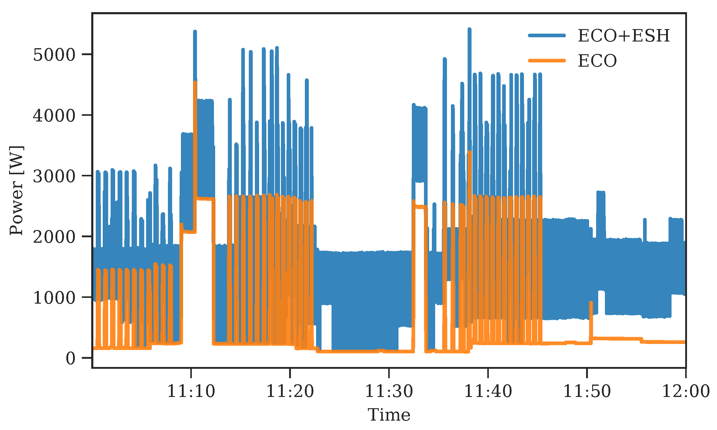
As shown in Figure 2, the aggregated power signal is generated by adding considerable power disturbances to the power consumption of the space heaters. Considering our approach to identifying ESHs, the disturbance is an unconcerned information level to uncover, presented in the aggregated signal that challenges the load disaggregation ambition. Accordingly, the unwanted information in terms of disturbances can be utilized to evaluate the robustness of the exploited mechanism to achieve an acceptable ESH power consumption estimation as the fruit of the disaggregation process. In our case study, the considered disturbance is a real aggregated signal of a house with several appliances accounting for an extensive number of events, which can itself be an exhausting NILM problem. Consequently, such a signal is suitable to be added to the ESH total aggregated load for examining the algorithm’s robustness. As a result, we utilized the ECO database and consider the data of a day with a high event rate of appliances, including one refrigerator, one freezer, one dishwasher, and one stove, as well as other minor appliances [46]. Subsequently, the ECO aggregated data was added to the ESH power profiles measured during one day. It is noted that the provided disturbance suggests a high power consumption that is comparable with the ESH’s notable energy usage.
In Figure 3, it can be observed that the disaggregated ESH power profile defined by the red curve is close to the measured ground-truth power profile, even if several other appliances are included in the original aggregated signal. In fact, the computed accuracy metric is higher than at 8 Hz. This result suggests the effectiveness of the proposed DHMM parameter estimation process.
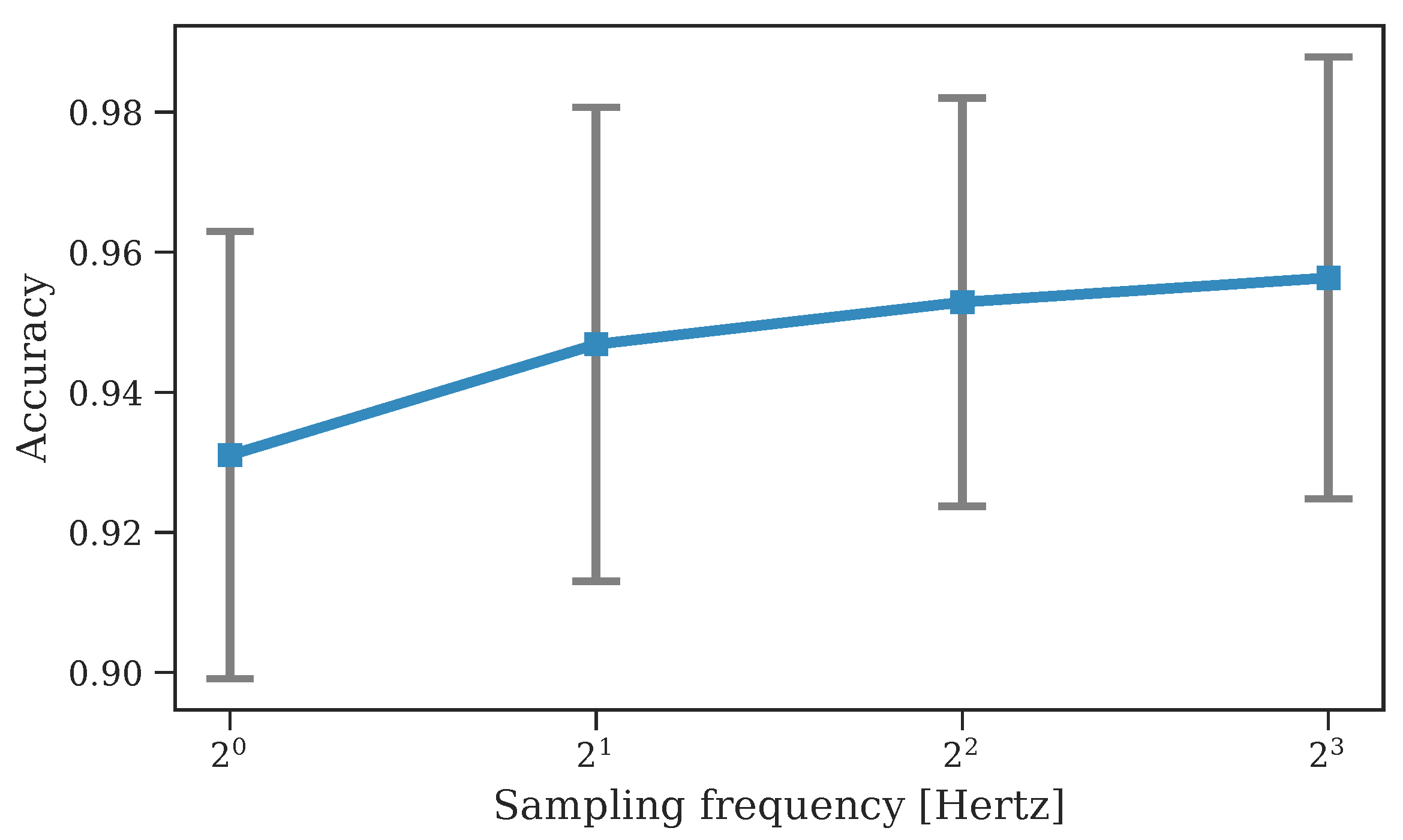
The impact of the sampling frequency on the disaggregation accuracy is demonstrated in Figure 4. It can be seen that the value increases with respect to the sampling frequency. With four electric heaters, the value is greater than while the sampling frequency is higher than 1 Hz according to the red curve. These results indicate the promise of the proposed approach to achieve a valid disaggregation practice even if the power profile is complex, with several electronic thermostats.
6.2. Comparative Study for Evaluating the One-at-a-Time Assumption
Moreover, our experimental and comparative study aims to provide the weaknesses of commonly used NILM approaches based on the well-known Hart method [10,19] in order to highlight the contribution of the DHMM aspect. Using the same method of combining the ECO-dataset aggregated power profile with electric heater power profiles (see Figure 2), we have performed the disaggregation of the refrigerator power profile. With no electric heater power profile and using the NILM method presented in [10], the refrigerator power is close to the ground-truth power profile during the steady-state operation. For this comparative study, the disaggregation accuracy metric (Equation (12)) was used. Additionally, we calculated the performance of the ESH power profile detection using the F-score measure [10]:
The accuracy of the disaggregated electric energy consumption is also estimated by the ratio between the estimated energy and ground-truth energy using the following equation:
Figure 5 illustrates that the computed metric is greater than when only conventional loads are presented in the aggregated profile. However, as the number of electric heater power profiles involved in the aggregated power profile increases, the disaggregation performance decreases exponentially and reaches with only four heaters, defined by the red curve. On the other hand, as shown in Figure 4, the proposed DHMM approach utilized to disaggregate the ESH load profile can maintain a remarkable performance of at an 8 Hz sampling frequency. The conducted scenario demonstrates the impracticality of recent NILM approaches based on the one-at-a-time assumption when low sampling frequencies are used.
7. Conclusions
In this work, we have presented a probabilistic approach to non-intrusively disaggregate ESH power profiles. The proposed disaggregation system uses a difference factorial hidden Markov model (DFHMM) to process active power changes in the aggregated signal. Furthermore, we have used a compositional Markovian modeling aspect based on the Kronecker representation, which allows us to construct ESH super-state models. Because underlying transition matrices involved in the overall DHMM framework were required, we proposed a simple and intuitive method to integrate the prior ESH parameters in the modeling process. The validation was performed using experimental data from our laboratory and the public ECO dataset. In addition, the comparative study between our approach and a commonly used Hart-based concept has indicated the efficacy of our proposed method to significantly improve the ESH power profile disaggregation performance. Finally, we have demonstrated the impact of the sampling frequency on the disaggregation performance as well as the robustness and efficacy of the proposed approach.
Acknowledgments
This work was supported by Laboratoire des technologies de l’énergie (LTE) d’Hydro-Québec, the Natural Science and Engineering Research Council of Canada and the Foundation UQTR.
Author Contributions
Nilson Henao proposed and implemented the methodology. Sousso Kelouwani validated the model and analyzed the data. Kodjo Agbossou was responsible for the direction of the project and contributed in designing the methodology. Michael Fournier provided feedback on the experimental work and data interpretation. Saeed Hosseini contributed to the results’ analysis and written discussion. All authors read and approved the final manuscript.
Conflicts of Interest
The authors declare no conflict of interest.
Abbreviations
The following abbreviations are used in this manuscript:
| NILM | Non-intrusive load monitoring |
| HMM | Hidden Markov model |
| DHMM | Difference HMM |
| FHMM | Factorial HMM |
| DFHMM | Difference FHMM |
| ESH | Electric space heating |
| RMS | Root-mean-square |
| AC | Alternative current |
| ML | Machine learning |
| ECO | Electricity Consumption and Occupancy |
| MAP | Maximum a Posteriori |
| AFAMAP | Additive Factorial Approximate MAP |
| MCMC | Markov chain Monte Carlo |
References
- Ma, Y.; Kelman, A.; Daly, A.; Borrelli, F. Predictive Control for Energy Efficient Buildings with Thermal Storage: Modeling, Stimulation, and Experiments. IEEE Control Syst. 2012, 32, 44–64. [Google Scholar] [CrossRef]
- Good, N.; Zhang, L.; Navarro-Espinosa, A.; Mancarella, P. Physical modeling of electro-thermal domestic heating systems with quantification of economic and environmental costs. In Proceedings of the IEEE Eurocon 2013, Zagreb, Croatia, 1–4 July 2013; pp. 1164–1171. [Google Scholar]
- Javed, A.; Larijani, H.; Ahmadinia, A.; Emmanuel, R. Modelling and optimization of residential heating system using random neural networks. In Proceedings of the 2014 IEEE International Conference on Control Science and Systems Engineering, Yantai, China, 29–30 December 2014; pp. 90–95. [Google Scholar]
- Egarter, D.; Sobe, A.; Elmenreich, W. Evolving non-intrusive load monitoring. In Lecture Notes in Computer Science; Including Subseries Lecture Notes in Artificial Intelligence and Lecture Notes in Bioinformatics; Springer: Vienna, Austria, 2013; Volume 7835 LNCS, pp. 182–191. [Google Scholar]
- Du, L.; Member, S.; Restrepo, J.A.; Yang, Y.; Harley, R.G.; Habetler, T.G. Nonintrusive, Self-Organizing, and Probabilistic Classification and Identification of Plugged-In Electric Loads. IEEE Trans. Smart Grid 2013, 4, 1371–1380. [Google Scholar] [CrossRef]
- Kramer, O.; Wilken, O.; Beenken, P.; Hein, A.; Klingenberg, T.; Meinecke, C.; Raabe, T.; Sonnenschein, M.; Hüwel, A. On Ensemble Classifiers for Nonintrusive Appliance Load Monitoring. Hybrid Artif. Intell. Syst. 2012, 7208, 322–331. [Google Scholar]
- Figueiredo, M.; de Almeida, A.; Ribeiro, B. Home electrical signal disaggregation for non-intrusive load monitoring (NILM) systems. Neurocomputing 2012, 96, 66–73. [Google Scholar] [CrossRef]
- Chang, H.H. Load identification of non-intrusive load-monitoring system in smart home. WSEAS Trans. Syst. 2010, 9, 498–510. [Google Scholar]
- Ducange, P.; Marcelloni, F.; Antonelli, M. A Novel Approach Based on Finite-State Machines with Fuzzy Transitions for Nonintrusive Home Appliance Monitoring. IEEE Trans. Ind. Inform. 2014, 10, 1185–1197. [Google Scholar] [CrossRef]
- Zhao, B.; Stankovic, L.; Stankovic, V. On a Training-Less Solution for Non-Intrusive Appliance Load Monitoring Using Graph Signal Processing. IEEE Access 2016, 4, 1784–1799. [Google Scholar] [CrossRef]
- Kim, H.; Marwah, M.; Arlitt, M.F.; Lyon, G.; Han, J. Unsupervised Disaggregation of Low Frequency Power Measurements. In Proceedings of the 11th SIAM International Conference on Data Mining, Mesa, AZ, USA, 28–30 April 2011; pp. 747–758. [Google Scholar]
- Srinivasarengan, K.; Goutam, Y.; Chandra, M.G.; Kadhe, S. A Framework for Non Intrusive Load Monitoring Using Bayesian Inference. In Proceedings of the 2013 Seventh International Conference on Innovative Mobile and Internet Services in Ubiquitous Computing, Taichung, Taiwan, 3–5 July 2013; pp. 427–432. [Google Scholar]
- Zeifman, M. Disaggregation of home energy display data using probabilistic approach. IEEE Trans. Consum. Electron. 2012, 58, 23–31. [Google Scholar]
- Zoha, A.; Gluhak, A.; Imran, M.A.; Rajasegarar, S. Non-intrusive load monitoring approaches for disaggregated energy sensing: A survey. Sensors 2012, 12, 16838–16866. [Google Scholar] [CrossRef] [PubMed] [Green Version]
- Parson, O.; Ghosh, S.; Weal, M.; Rogers, A. An Unsupervised Training Method for Non-Intrusive Appliance Load Monitoring. Artif. Intell. 2014, 217, 1–19. [Google Scholar] [CrossRef]
- Parson, O. Using Hidden Markov Model Variants for Non-intrusive Appliance Load Monitoring from Smart Meter Data; Technical report; University of Southampton: Southampton, UK, 2012. [Google Scholar]
- Egarter, D.; Pöchacker, M.; Elmenreich, W. Complexity of Power Draws for Load Disaggregation. arXiv, 2015; arXiv:1501.02954. Available online: https://arxiv.org/abs/1501.02954(accessed on 16 May 2016).
- Guedri, M.E.; D’Urso, G.; Lajaunie, C.; Fleury, G. RJMCMC point process sampler for single sensor source separation: An application to electric load monitoring. In Proceedings of the IEEE 17th European Signal Processing Conference EUSIPCO, Glasgow, UK, 24–28 August 2009; pp. 1062–1066. [Google Scholar]
- Henao, N.; Agbossou, K.; Kelouwani, S.; Dube, Y.; Fournier, M. Approach in Nonintrusive Type I Load Monitoring Using Subtractive Clustering. IEEE Trans. Smart Grid 2015, 8, 812–821. [Google Scholar] [CrossRef]
- Froehlich, J.; Larson, E.; Gupta, S.; Cohn, G.; Reynolds, M.; Patel, S. Disaggregated End-Use Energy Sensing for the Smart Grid. IEEE Pervasive Comput. 2011, 10, 28–39. [Google Scholar] [CrossRef]
- Makonin, S. Approaches to Non-Intrusive Load Monitpring (NILM) in the Home; Technical report; BTech, British Columbia Institute of Technology: Burnaby, BC, Canada, 2012. [Google Scholar]
- Batra, N.; Parson, O.; Berges, M.; Singh, A.; Rogers, A. A comparison of non-intrusive load monitoring methods for commercial and residential buildings. arXiv, 2014; arXiv:1408.6595 [cs.SY]. Available online: https://arxiv.org/abs/1408.6595(accessed on 24 April 2015).
- Zeifman, M.; Akers, C.; Roth, K. Nonintrusive appliance load monitoring: Review and outlook. IEEE Trans. Consum. Electron. 2011, 57, 76–84. [Google Scholar] [CrossRef]
- Hassan, T.; Javed, F.; Arshad, N. An Empirical Investigation of V-I Trajectory Based Load Signatures for Non-Intrusive Load Monitoring. IEEE Trans. Smart Grid 2013, 5, 870–878. [Google Scholar] [CrossRef]
- Wong, Y.F.; Ahmet Sekercioglu, Y.; Drummond, T.; Wong, V.S. Recent approaches to non-intrusive load monitoring techniques in residential settings. In Proceedings of the 2013 IEEE Computational Intelligence Applications in Smart Grid (CIASG), Singapore, 16–19 April 2013; pp. 73–79. [Google Scholar]
- Akbar, M.; Khan, Z.A. Modified Nonintrusive Appliance Load Monitoring For Nonlinear Devices. In Proceedings of the 2007 IEEE International Multitopic Conference, Lahore, Pakistan, 28–30 December 2007; pp. 1–5. [Google Scholar]
- Wang, Y.; Filippi, A.; Rietman, R.; Leus, G. Compressive Sampling for Non-Intrusive Appliance Load Monitoring (NALM) using Current Waveforms. In Proceedings of the Signal Processing, Pattern Recognition and Applications/ 779: Computer Graphics and Imaging (SPPRA 2012), Crete, Greece, 18–20 June 2012; pp. 2–8. [Google Scholar]
- Kolter, J.Z.; Jaakkola, T. Approximate Inference in Additive Factorial HMMs with Application to Energy Disaggregation. JMLR Proc. 2012, 22, 1472–1482. [Google Scholar]
- Zoha, A.; Gluhak, A.; Nati, M.; Imran, M.A. Low-power appliance monitoring using Factorial Hidden Markov Models. In Proceedings of the 2013 IEEE Eighth International Conference on Intelligent Sensors, Sensor Networks and Information Processing, Melbourne, VIC, Australia, 2–5 April 2013; pp. 527–532. [Google Scholar]
- Ghahramani, Z.; Jordan, M.I. Factorial Hidden Markov Models. Mach. Learn. 1997, 29, 245–273. [Google Scholar] [CrossRef]
- Monin Nylund, J.-A. Semi-Markov modelling in a Gibbs sampling algorithm for NIALM. Masters Thesis, Royal Institute of Technology, Stockholm, Sweden, 2013. [Google Scholar]
- Sanquer, M.; Chatelain, F.; El-Guedri, M.; Martin, N. A reversible jump MCMC algorithm for Bayesian curve fitting by using smooth transition regression models. In Proceedings of the 2011 IEEE International Conference on Acoustics, Speech and Signal Processing (ICASSP), Prague, Czech Republic, 22–27 May 2011; pp. 3960–3963. [Google Scholar]
- Chen, S.-H.; Ip, E.H. Behaviour of the Gibbs sampler when conditional distributions are potentially incompatible. J. Stat. Comput. Sim. 2015, 85, 3266–3275. [Google Scholar] [CrossRef] [PubMed]
- Lange, H.; Berg, M. Efficient Inference in Dual-Emission FHMM for Energy Disaggregation. In Proceedings of the Artificial Intelligence for Smart Grids and Smart Buildings, Phoenix, AZ, USA, 25–30 January 2015; pp. 248–254. [Google Scholar]
- Makonin, S.; Popowich, F.; Bajic, I.V.; Gill, B.; Bartram, L. Exploiting HMM Sparsity to Perform Online Real-Time Nonintrusive Load Monitoring. IEEE Trans. Smart Grid 2016, 7, 2575–2585. [Google Scholar] [CrossRef]
- Hart, G.W. Nonintrusive appliance load monitoring. Proc. IEEE 1992, 80, 1870–1891. [Google Scholar] [CrossRef]
- Hassan, T.; Javed, F.; Arshad, N. An Empirical Investigation of V-I Trajectory Based Load Signatures for Non-Intrusive Load Monitoring. IEEE Trans. Smart Grid 2014, 5, 870–878. [Google Scholar] [CrossRef]
- Chang, H.H.; Lian, K.L.; Su, Y.C.; Lee, W.J. Power-Spectrum-Based Wavelet Transform for Nonintrusive Demand Monitoring and Load Identification. IEEE Trans. Ind. Appl. 2014, 50, 2081–2089. [Google Scholar] [CrossRef]
- Jacobs, R.A.; Jiang, W.; Tanner, M.A. Factorial Hidden Markov Models and the Generalized Backfitting Algorithm. Neural Comput. 2002, 14, 2415–2437. [Google Scholar] [CrossRef] [PubMed]
- Sankara, A. Energy Disaggregation in NIALM Using Hidden Markov Models. Ph.D. Thesis, Missouri University of Science and Technology, Rolla, MO, USA, 2015. [Google Scholar]
- Tuğrul, D. Analyzing markov chains based on kronecker products. Computer 2012, 4047, 279–300. [Google Scholar]
- Parson, O. Unsupervised Training Methods for Non-intrusive Appliance Load Monitoring from Smart Meter Data. Ph.D. Thesis, University of Southampton, Southampton, UK, 2014. [Google Scholar]
- Roberts, G.O.; Rosenthal, J.S. Surprising Convergence Properties of Some Simple Gibbs Samplers under Various Scans. Int. J. Stat. Probab. 2015, 5, 51. [Google Scholar] [CrossRef]
- Henao, N.; Kelouwani, S.; Agbossou, K.; Dube, Y. Active power load modeling based on uncertainties for Non Intrusive Load Monitoring. In Proceedings of the 2016 IEEE 25th International Symposium on Industrial Electronics (ISIE), Santa Clara, CA, USA, 8–10 June 2016; pp. 684–689. [Google Scholar]
- Makonin, S.; Popowich, F. Nonintrusive load monitoring (NILM) performance evaluation. Energy Effic. 2015, 8, 809–814. [Google Scholar] [CrossRef]
- Beckel, C.; Kleiminger, W.; Cicchetti, R.; Staake, T.; Santini, S. The ECO data set and the performance of non-intrusive load monitoring algorithms. In Proceedings of the 1st ACM Conference on Embedded Systems for Energy-Efficient Buildings (BuildSys’14), Memphis, TN, USA, 3–6 November 2014; pp. 80–89. [Google Scholar]
Figure 1.
Number of iterations until convergence of a Gibbs sampler for joint hidden states.
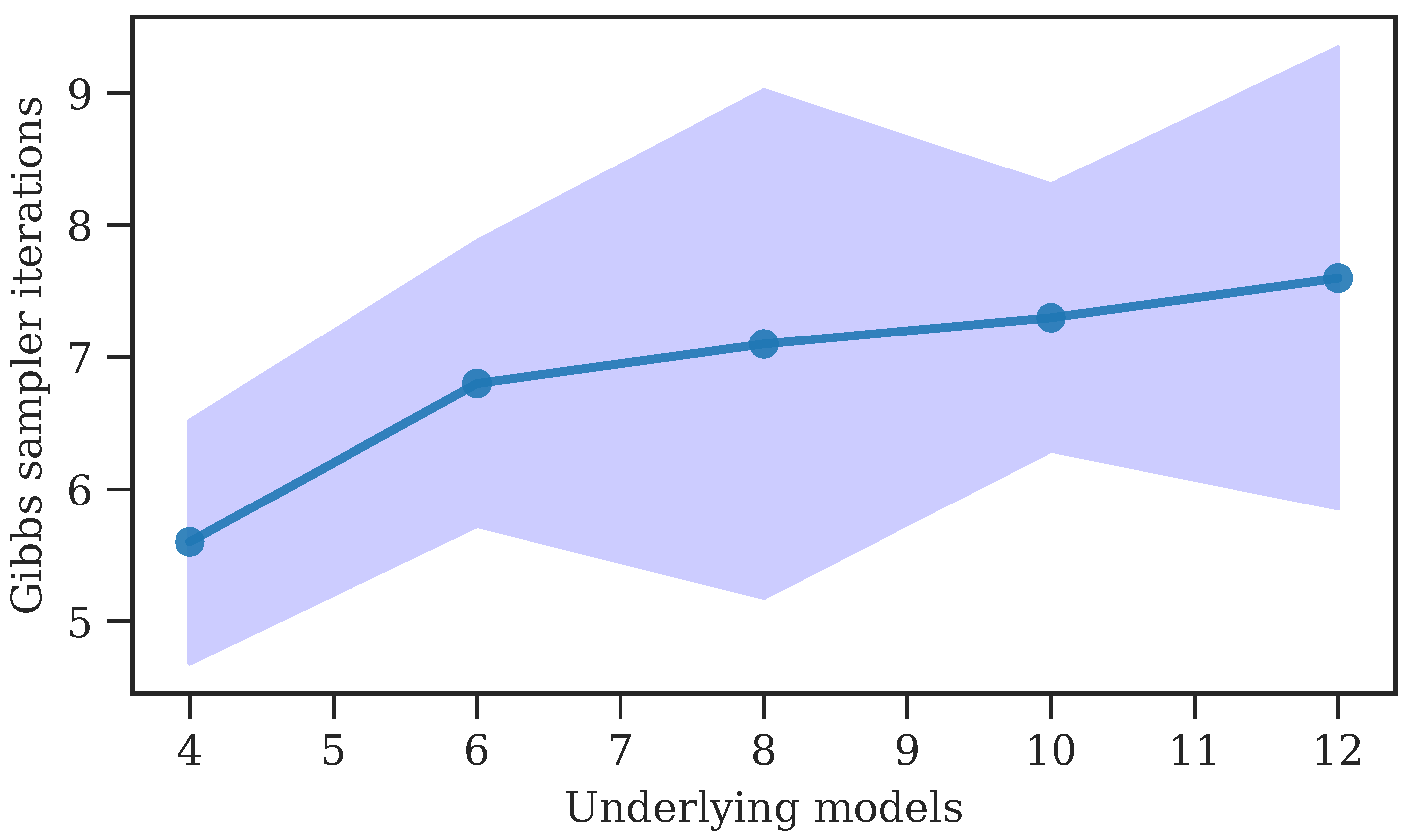
Figure 2.
Aggregated power profiles of electric heater appliances and ECO dataset.

Figure 3.
Disaggregated power profile of four baseboards.
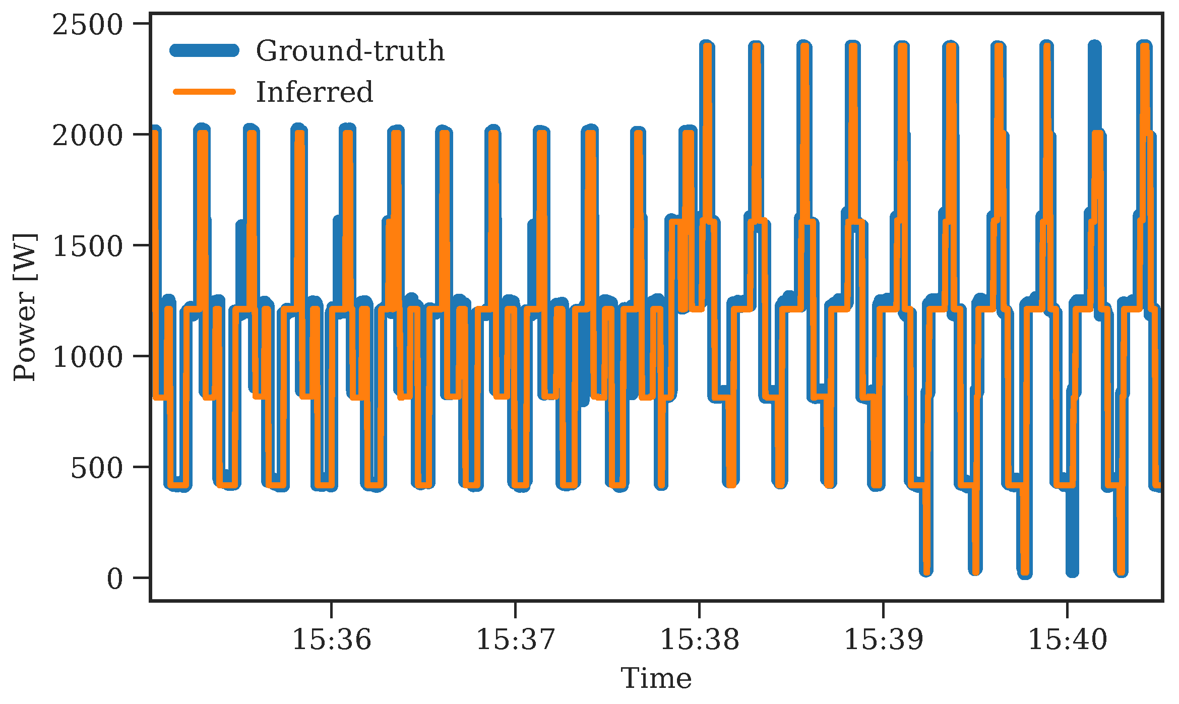
Figure 4.
Performance of electric space heater (ESH) power disaggregation at different sampling frequencies.
Figure 4.
Performance of electric space heater (ESH) power disaggregation at different sampling frequencies.

Figure 5.
Disaggregation performance in the presence of electric heater instances.


Table 1.
Parameter set-up of electric space heater (ESH) disaggregation practice.
| Parameter | Value |
|---|---|
| Commutation period, | 16 s |
| Baseboards’ power at 240 Volts | W |
| Off-state average power | W |
| Off-state power standard deviation | 6 W |
| Coefficient of variation, | 0.015 |
| Stopping Gibbs sampling, | 0.01 |
© 2018 by the authors. Licensee MDPI, Basel, Switzerland. This article is an open access article distributed under the terms and conditions of the Creative Commons Attribution (CC BY) license (http://creativecommons.org/licenses/by/4.0/).
Share and Cite
MDPI and ACS Style
Henao, N.; Agbossou, K.; Kelouwani, S.; Hosseini, S.S.; Fournier, M. Power Estimation of Multiple Two-State Loads Using A Probabilistic Non-Intrusive Approach. Energies 2018, 11, 88. https://doi.org/10.3390/en11010088
AMA Style
Henao N, Agbossou K, Kelouwani S, Hosseini SS, Fournier M. Power Estimation of Multiple Two-State Loads Using A Probabilistic Non-Intrusive Approach. Energies. 2018; 11(1):88. https://doi.org/10.3390/en11010088
Chicago/Turabian StyleHenao, Nilson, Kodjo Agbossou, Sousso Kelouwani, Sayed Saeed Hosseini, and Michael Fournier. 2018. "Power Estimation of Multiple Two-State Loads Using A Probabilistic Non-Intrusive Approach" Energies 11, no. 1: 88. https://doi.org/10.3390/en11010088
Note that from the first issue of 2016, this journal uses article numbers instead of page numbers. See further details here.