Long-Term Battery Voltage, Power, and Surface Temperature Prediction Using a Model-Based Extreme Learning Machine †

1
Department of Chemical and Biological Engineering, The Hong Kong University of Science and Technology, Clear Water Bay, Kowloon, Hong Kong, China
2
Guangzhou HKUST Fok Ying Tung Research Institute, Guangzhou 510000, China
*
Author to whom correspondence should be addressed.
†
A short version of the paper was presented at ISEV2017 on 26–29 July in Sweden. This paper is a substantial extension of the short version of the conference paper.
Energies 2018, 11(1), 86; https://doi.org/10.3390/en11010086
Submission received: 23 November 2017
/
Revised: 9 December 2017
/
Accepted: 11 December 2017
/
Published: 3 January 2018
(This article belongs to the Special Issue The International Symposium on Electric Vehicles (ISEV2017))
Abstract
:A battery’s state-of-power (SOP) refers to the maximum power that can be extracted from the battery within a short period of time (e.g., 10 s or 30 s). However, as its use in applications is growing, such as in automatic cars, the ability to predict a longer usage time is required. To be able to do this, two issues should be considered: (1) the influence of both the ambient temperature and the rise in temperature caused by Joule heat, and (2) the influence of changes in the state of charge (SOC). In response, we propose the use of a model-based extreme learning machine (Model-ELM, MELM) to predict the battery future voltage, power, and surface temperature for any given load current. The standard ELM is a kind of single-layer feedforward network (SLFN). We propose using a set of rough models to replace the active functions (such as logsig()) in the ELM for better generalization performance. The model parameters and initial SOC in these “rough models” are randomly selected within a given range, so little prior knowledge about the battery is required. Moreover, the identification of the complex nonlinear system can be transferred into a standard least squares problem, which is suitable for online applications. The proposed method was tested and compared with RLS (Recursive Least Square)-based methods at different ambient temperatures to verify its superiority. The temperature prediction accuracy is higher than ±1.5 °C, and the RMSE (Root Mean Square Error) of the power prediction is less than 0.25 W. It should be noted that the accuracy of the proposed method does not rely on the accuracy of the state estimation such as SOC, thereby improving its robustness.
1. Introduction
Electric vehicles (EV) and Plug-in hybrid electric vehicles (PHEV) are transportation solutions to the worldwide energy and environmental crisis [1,2,3], in which lithium-based batteries are commonly used as the only power source [4,5]. Normally, a battery management system (BMS) is a requisite to monitor and control the working status (such as temperature and voltage) of these cells, which, in return, keeps the EVs safe and extends the battery pack’s lifespan [6,7]. Among the most important variables for a BMS to track is the maximum power that can be properly extracted from (or charged into) the battery within a short period of time (e.g., 10 s or 30 s) [8]. This is defined as the battery’s state of power (SOP). The SOP can influence the accelerating, braking, and climbing performance of an EV, which is critical to the user experience. The ability to predict this has gained the interest of many researchers.
The methods relating to SOP prediction can be categorized into two types, namely, offline determination and online calculation. The dominant offline approach to determine the static SOP is the HPPC (hybrid pulse power characterization) developed by the Idaho National Engineering & Environmental Laboratory [9]. However, this is a sub-optimal approach and can only be tested in a lab environment. Compared with hybrid pulse power characterization (HPPC), the online calculation of SOP is more competitive. The general idea of the online approach is to firstly obtain a battery’s model, and then use this model to calculate the voltage response of a given current to obtain the corresponding power [10,11]. Since the battery performance is strongly related with its internal states, the actual SOP prediction process is usually combined with the estimation of the battery’s open circuit voltage (OCV), state of charge (SOC), polarization voltage, and so on [11,12]. Understanding that the battery should not be overused, the predicted maximum output power should thus satisfy a set of constraints such as those relating to SOC [13], state of energy (SOE)[14], voltage [15], and temperature [16]. To balance the accuracy and computational cost, the Thevenin model is most commonly used in more recent publications [17,18,19,20]. It is also suggested that a diffusion model should be further considered if the temperature is low [21].
However, it should be noted that most of the existing SOP estimation only covers a short period of time, up to a few hundreds of seconds. With increasing user demand, a much longer predication time is required. In other words, we want to know in advance if a battery is still within its safe operating window [22] after having run a certain load condition for a few hours. To fulfill this task, some issues should be further considered:
- Temperature: the battery performance and its safety can be influenced significantly by temperature [23,24,25]. When the prediction time is short, it is reasonable to set the battery temperature as the surface temperature. However, for long-term prediction, the battery temperature may change due to the accumulation of the Joule heat [16,26]. Therefore, the battery’s future temperature should be predicted before its long-term voltage and power.
- SOC: the battery OCV, and thus the terminal voltage, is strongly related to the SOC [27,28,29]. For short-term prediction, as long as the capacity change is not significant, the SOC and OCV can be regarded as a constant number [30], which is beneficial for online calculations. However, the SOC change can no longer be neglected if we are doing long-term predictions. It should be noted that estimating the SOC online at changing temperatures is not only difficult, but may also be computationally complex [23,31]. Unfortunately, without an accurate SOC estimation, the initial SOC for the long-term open-loop prediction is no longer accurate, which will lead to a drift in the predicted voltage.
In response to the above problems, we propose a model-based extreme learning machine (MELM) method to model the battery and predict the future temperature, voltage, and power. By doing so, we can compare these values with the corresponding operating limitations. extreme learning machine (ELM) is a type of single layer feedforward network (SLFN) with better generalization performance than the Back Propagation back propagation (BP)neural network [32,33]. We propose replacing the active functions by a set of models to further enhance the long-term prediction performance. To predict the future temperature, a first order plus delay model is proposed, and to predict the battery’s future voltage or power, an enhanced Thevenin model, in which each parameter changes with the temperature, is proposed. The online identification of some model parameters in this case, such as the time delay or temperature coefficients, can be difficult and computationally complex. To overcome this problem, we rely on the advantages of the ELM method: first, randomly select these parameters within a given range for each model in the network and, second, integrate these models with random parameters using a standard least squares (LS) algorithm. The proposed method is verified and shown to be superior with different load conditions at different temperatures.
The remainder of this paper is organized as follows: the algorithms—including the standard ELM, proposed MELM, temperature model and enhanced Thevenin model—are introduced in Section 2; the experimental configurations and results are introduced in Section 3; and the conclusions are noted in Section 4.
2. Algorithm Design
2.1. Conventional Extreme Learning Machine
ELM is a type of single layer feedforward network (SLFN) proposed by Huang [32], and its structure is similar to that of the three-layer neural network shown in Figure 1.
However, its training procedure is very different to the BP neural network [33,34]. Referring to Figure 1, the output of the network can be expressed as:
where x(·) is the uniformed input data with length L, a(·, ·) is the input weight function with the size N × L, b(·) is the input bias, and W(·) stands for the output weight matrix with the length N. The matrix parameters in matrix a = a(i, j) and b = b(i, j) are randomly selected and the active function in ELM is s-function such as logsig() or tanh() function. Equation (1) in the matrix form:
where , and . In this way, if we have S training samples, we can calculate the optimal W matrix using the following method:
where H = [h(1,:), h(2,:), …, h(S,:)]T, and Y = [y(1), y(2), … y(S)]T. This method can guarantee that Wop is the minimal norm least squares solution. This solution can also be obtained using its recursive form, called recursive least squares (RLS), as shown in the following Table 1.
In this table, λ is the forgetting factor, P is the inverse correlation matrix of the input signal, Y is the real system output, and h·W is the RLS output. The weight W is updated using the error between these two outputs in step 4, where the updated gain, K, is calculated in step 2. When λ = 1, the algorithm provides a recursive way to calculate Wop in equation (3) and when λ < 1, the RLS output relies more on the new measurements and tend to “forget” the old measurements.
2.2. Model-Based Extreme Learning Machine
In this section, we propose replacing the active functions in the ELM with a set of sub-models. What is generated is called the Model-ELM (MELM) method. An illustration of the MELM method is given in Figure 2.
In this diagram, the system output is the weighted sum of the N sub-model outputs, and the weight can be calculated using the online RLS method introduced above. The structure of the sub-models is pre-determined, while the model parameters are randomly selected within a given range (see also Section 2.3 and Section 3 for details). The benefits of using this MELM can be listed as follows:
- High model accuracy can be obtained without using complex sub-model structures. This can be beneficial when an accurate system model structure is not available. It should be noted that this is also a benefit of general data-driven methods [35].
- Generalization performance of SLFN can be improved. The conventional logsig() function is only sensitive to input when the input is close to zero; in other words, SLFN may not perform well if the testing data is far from the training data range [33,34]. An (even inaccurate) mechanism model does not have this limitation.
- The model can be represented in a parameter-distributed way through this MELM. In other words, the system is represented by a lot of sub-models with the same structure but different model parameters. A parameter-distributed model usually better describes the real system, as illustrated in Figure 3. The time delay for the heat transferred to the temperature sensor can be different to the heat generated in different parts of the batteries.
2.3. Model Structure
In this subsection, the selected model for MELM is introduced. We need two models, namely, the battery temperature model and battery equivalent circuit model.
2.3.1. Battery Temperature Model
In general, the battery temperature model consists of two elements: heat generation and heat dissipation. Therefore, a rough first-order temperature model considering time delay could have the following form:
where is the temperature difference between the battery surface and environment at time k. α describes the degrading rate of the temperature difference or possible entropy change due to chemical reactions [26], β describes the heat generation rate due to the Joule heat or possible entropy change due to chemical reactions, γ is used to distinguish the difference between charging and discharging, and delay represents the time delay between the current and temperature. In this model, α, β and delay are randomly selected within a given range, while γ is set to be 1 when discharging, and randomly selected within a given range when charging.
To obtain a reasonable limit range for the parameter changes, referenced α and β can be obtained in advance using the least squares method, the referenced delay can be obtained using the direct observation method, and the referenced γ for charging can be obtained by comparing the impedance when charging and discharging. The “given range” is a relatively wide neighborhood region of the referenced value (seen in Table 4 for further details). In this way, the output of the entire algorithm can be regarded as the weighted sum of the sub-model outputs, and the weight can be calculated using the LS method.
2.3.2. Battery Equivalent Circuit Model
First, the definition of SOC is given by:
where SOC0 is the initial state of charge, η is the Coulomb efficiency, which is usually treated as 1 for discharging, i is the current and Cn is the battery capacity. In this paper, the Thevenin model is adopted to describe a battery system: where Idischarge is the load current, and the subscript discharge means the current is positive when discharging, Ut is the terminal voltage of the battery, R0 is the ohmic resistance, Cp stands for the equivalent polarization capacitance and Rp is the polarization resistance over Cp, through which the relaxation effect during charging/discharging process can be simulated, Up is the voltage across the Cp, U0 is the voltage across the R0, and Uoc is the OCV of the battery. Based on the requirement of the accuracy and computational complexity, these model parameters can be described in either time-varying fashion or time-invariant fashion.
If we re-write the above equations in a more abstract form by setting Up and SOC as the state variables, current as the input variable (positive when charging), and terminal voltage as output variable, then we have:
and its linearization at time k can be written as:
where wk and vk are independent, zero mean Gaussian noise, whose covariance matrix is Q and R, respectively. In this way, the detailed parameters in the equations can be given as follows:
where τ is the sampling time, which is selected as 1 s in this paper, and Cn is the capacity whose unit is A•sec.
In this paper, OCV are assumed to change with the SOC and temperature, and this relationship can be described by:
where lookup() means the corresponding look-up table, T stands for the battery surface temperature, and HY stands for the hysteresis and other uncertain initial states, which is set to 0 when the model parameters are obtained in an accurate way.
In this paper, the OCV–SOC relationship at different temperatures of the target battery is pre-determined, and other parameters such as Cn, R0, Cp, Rp, and HY are randomly selected within a given range at 25 °C. The referenced value of these parameters can be obtained using the least squares method and the “given range” is a wide neighborhood of the reference value (seen in Table 5 for further details), which is similar to the temperature prediction cases. When the temperature is not equal to 25 °C, the above stated parameters x (x = Cn, R0, Cp, Rp, or HY) are assumed to change linearly with temperature, i.e.,
where ci are coefficients. Similarly, these ci can be randomly selected within a given range for x = Cn, R0, Cp, Rp, or HY, respectively.
Unlike existing methods that try to estimate SOC using different kinds of algorithms, the uncertain initial SOCs of each sub-model are also randomly selected within the given range in the proposed method, and then determined by direct open-loop model iteration. This can not only save the computation, but also guarantee the diversity of the models. In other words, if we estimate the SOC, the SOC in each sub-model will converge to a similar value, reducing the model diversity. It should be noted that the model diversity is important for the MELM method, and is also a basic requirement of some Monto Carlo-based methods such as particle filters [23,38].
Similar to the temperature case, all the unknown parameters or states are randomly selected for each sub-model, and the output of the entire algorithm can be regarded as the weighted sum of the sub-model outputs. The weight can be calculated using the LS method.
2.4. Summary
The SOP is mainly limited by the voltage and temperature limitations. Therefore, its estimation can be transformed into a temperature and voltage prediction problem. If an accurate model and a correct initial state are available, the future battery temperature, terminal voltage, and corresponding power can be well predicted in an open loop fashion for any given future current load profile. The “accurate model” in this paper is obtained by the proposed MELM method, and the entire procedure of this method can be summarized by the following Table 2.
3. Experimental Result
3.1. Experimental Platform
3.2. Model Parameter Selection
In the following tests, the number of randomly generated models is 50, and the detailed model generation methods for temperature model and Thevenin model are provided separately as follows.
3.2.1. Temperature Model
In this paper, the battery temperature model parameters for programming are provided in Table 4.
It should be noted that the reference value is calculated using the LS method and the testing data. It is a good guideline for the determination of the parameter selection range; however, it is not necessary and the range can be determined using a datasheet or by calling on experience.
3.2.2. Thevenin Model
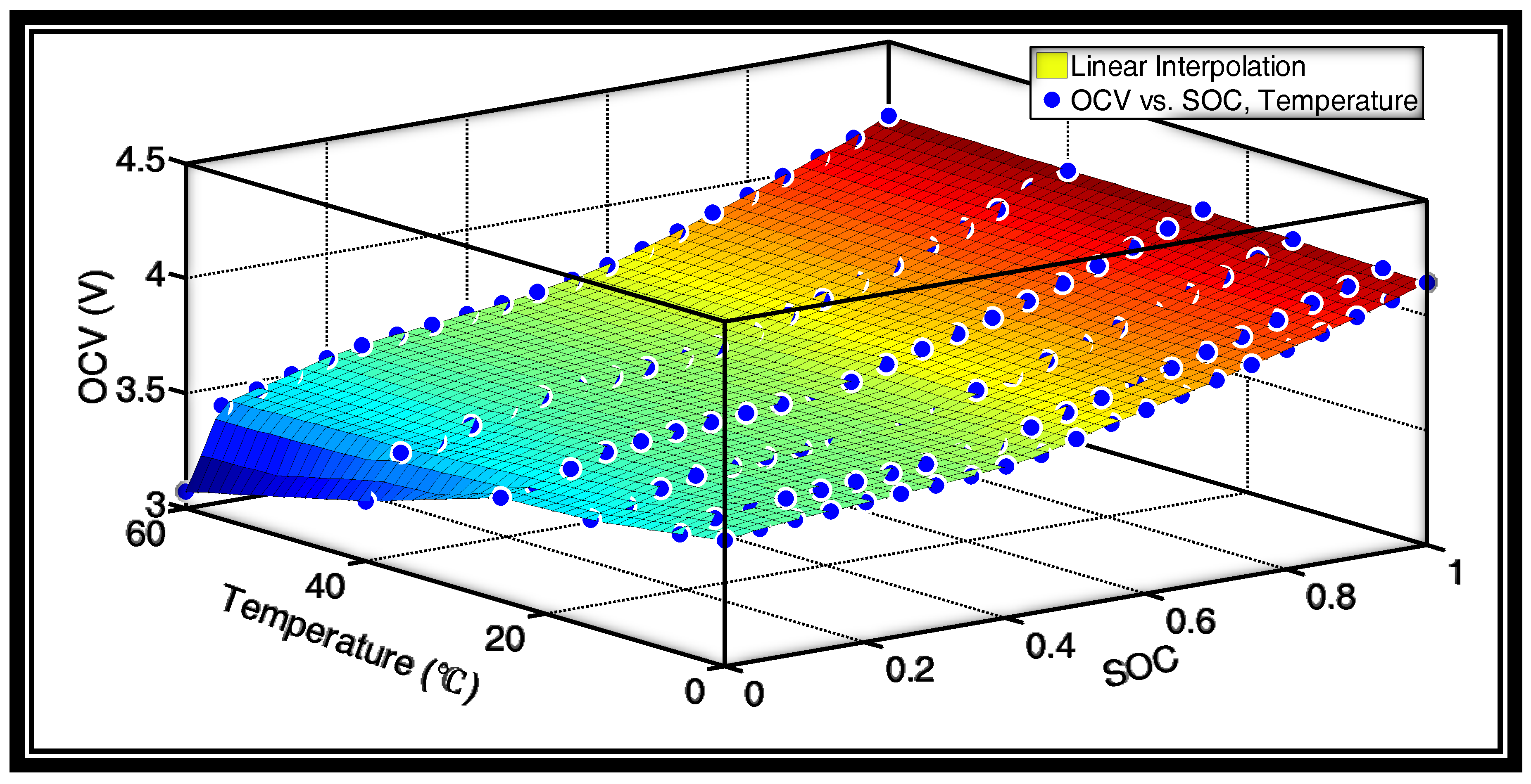
In this paper, the battery OCV–SOC relationship at different ambient temperatures is provided in Figure 6.
The corresponding model parameters at 25 °C, suggested temperature changing coefficients, and corresponding selected parameter ranges are provided in Table 5. The referenced model parameters in Table 5 are obtained using the least squares method; see [39] for details. The suggested ci values are obtained by conducting a linear fit between temperature and the corresponding identified model parameters.
Like the previous case, these referenced values can be a good guideline for parameter range determination, but they are not necessary. The parameter ranges may also be obtained from the datasheet or calling on experience. It should be noted that although an accurate OCV–SOC relationship at different temperatures is used in this paper (because it is not difficult to obtain), it is also not necessary for the proposed method. In fact, the HY term introduced in Equation (13) improves the model diversity.
3.3. Future Temperature and Power Prediction Results
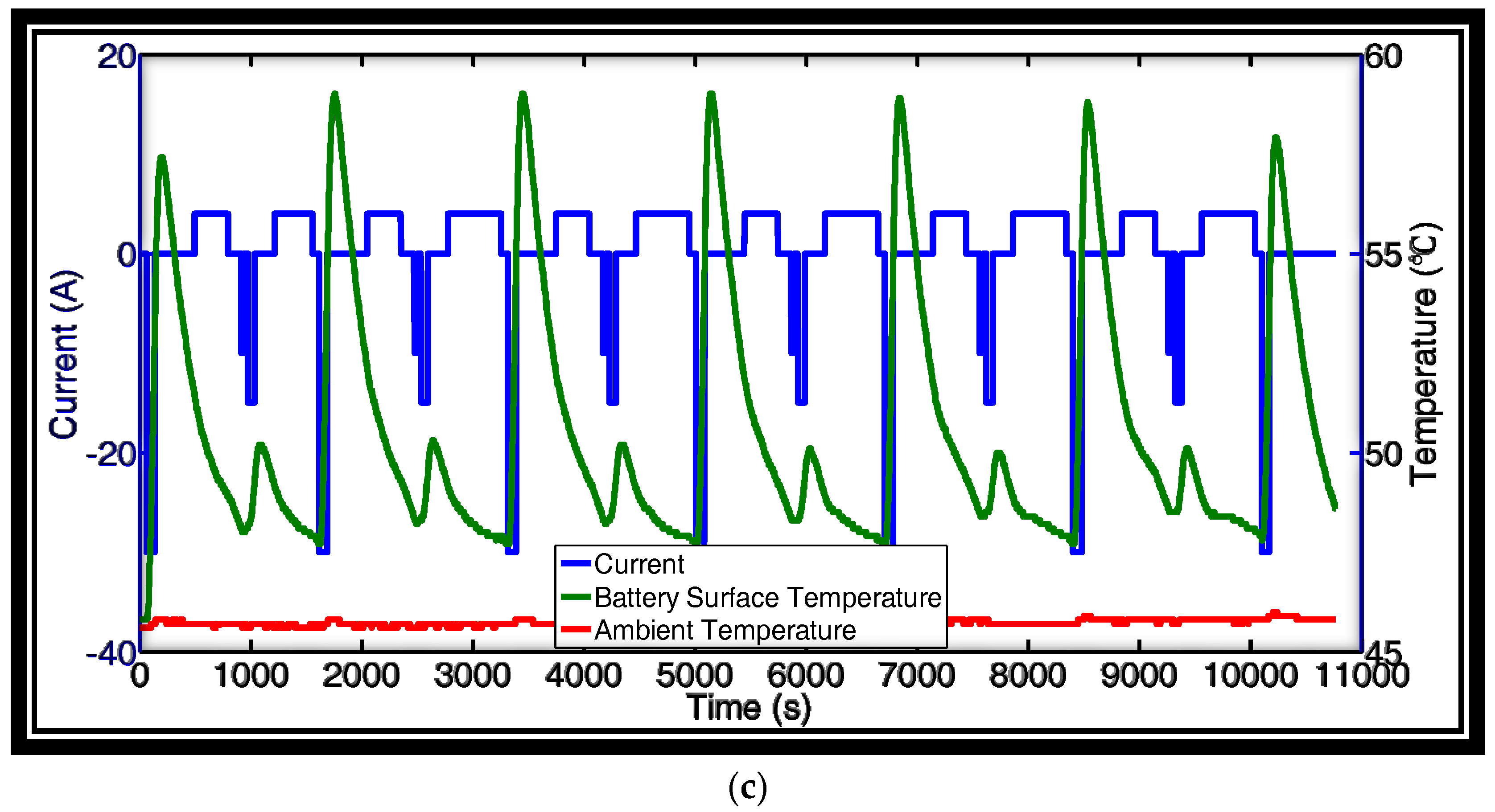
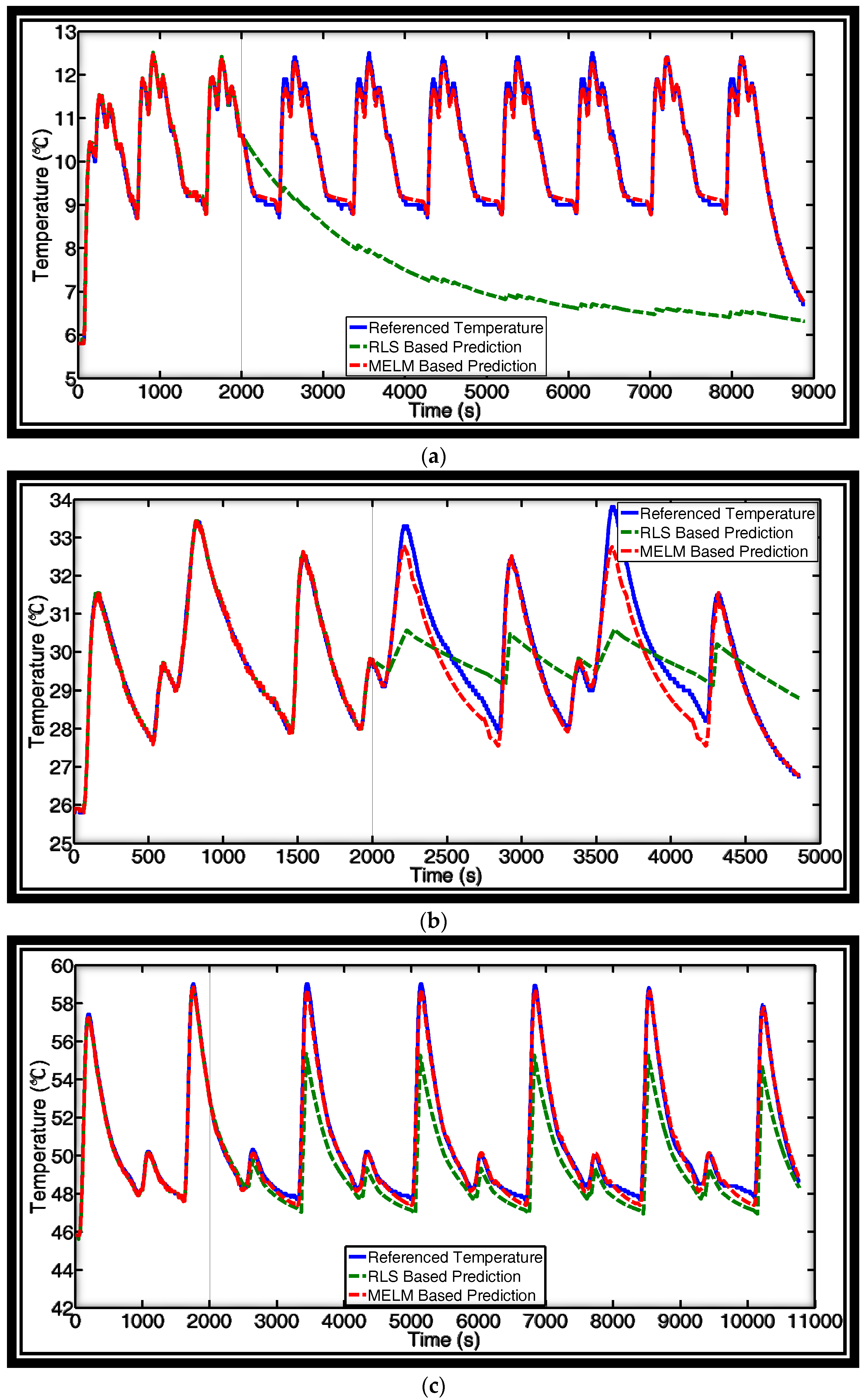
In this paper, the experiments are carried out at three different ambient temperatures: 5 °C, 25 °C, and 45 °C. The sampling frequency is 1 Hz. The selected load condition and the corresponding battery surface temperature response are shown in Figure 7. For all three conditions, we assume that we want to predict the battery’s future surface temperature, voltage, and power at 2000 s. In other words, we assumed that data corresponding to the first 2000 s are available, and we use these data to predict the voltage and temperature response from 2001 s to the end of the test in an open-loop fashion. Although we can predict any given load conditions, we have to predict the response of the load condition shown in Figure 7 to compare it with the real measurement and verify the method. The corresponding results are provided in the following sub-sections.
3.3.1. Temperature Prediction Result
In this paper, the proposed method is compared with a commonly used online RLS method, in which α and β are identified online, delay is selected as 50 s, and γ is set at 1. The results of the RLS method and the proposed MELM method are shown in Figure 8.
From this result, the RLS method may perform well, but the performance is not stable. The models used in the MELM have almost the same structure as the RLS-based method, and by combining these models together, the overall result improves greatly. This indicates that modeling the battery temperature model in a parameter-distributed way is promising. It should be noted that each model in the MELM method is not optimal, compared with the RLS-identified results, which, in turn, verifies the effectiveness of the MELM method. The RLS-based temperature method will not diverge if the identified system is inherently stable. For the MELM method, if each randomly generated model is stable, the overall result can be stable. This can be easily guaranteed by selecting a reasonable parameter range for MELM. It can also be seen that the temperature prediction error can be limited to ±1.5 °C using the proposed MELM method, which is quite accurate. The improvement of the generalization performance of the MELM method is discussed in the original conference version of this paper, in which the standard ELM model, MELM model, back propagation neural network (BPNN) model, lumped model, and first order plus time delay model are compared. The results obtained using training data with different sizes were also compared.
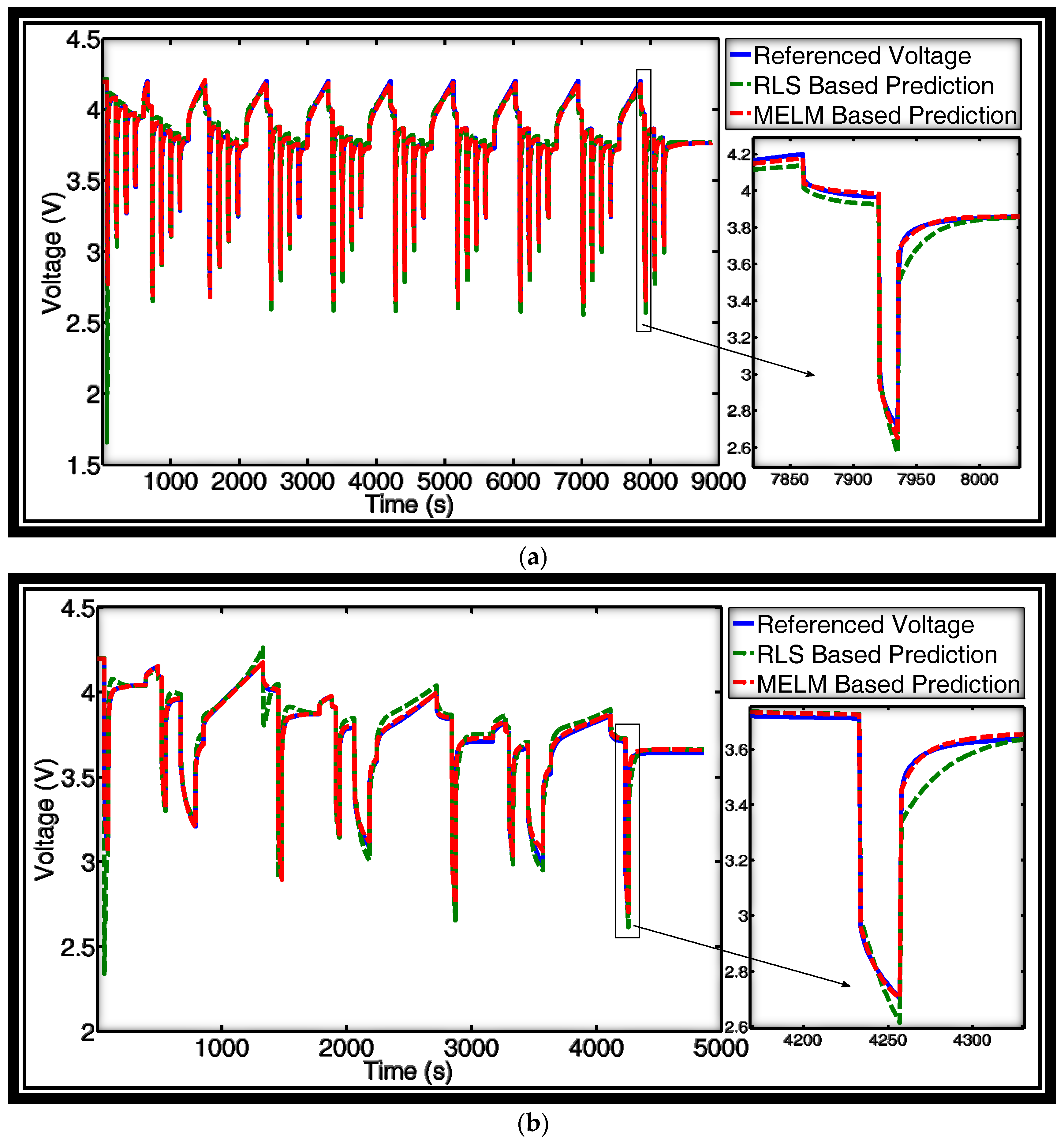
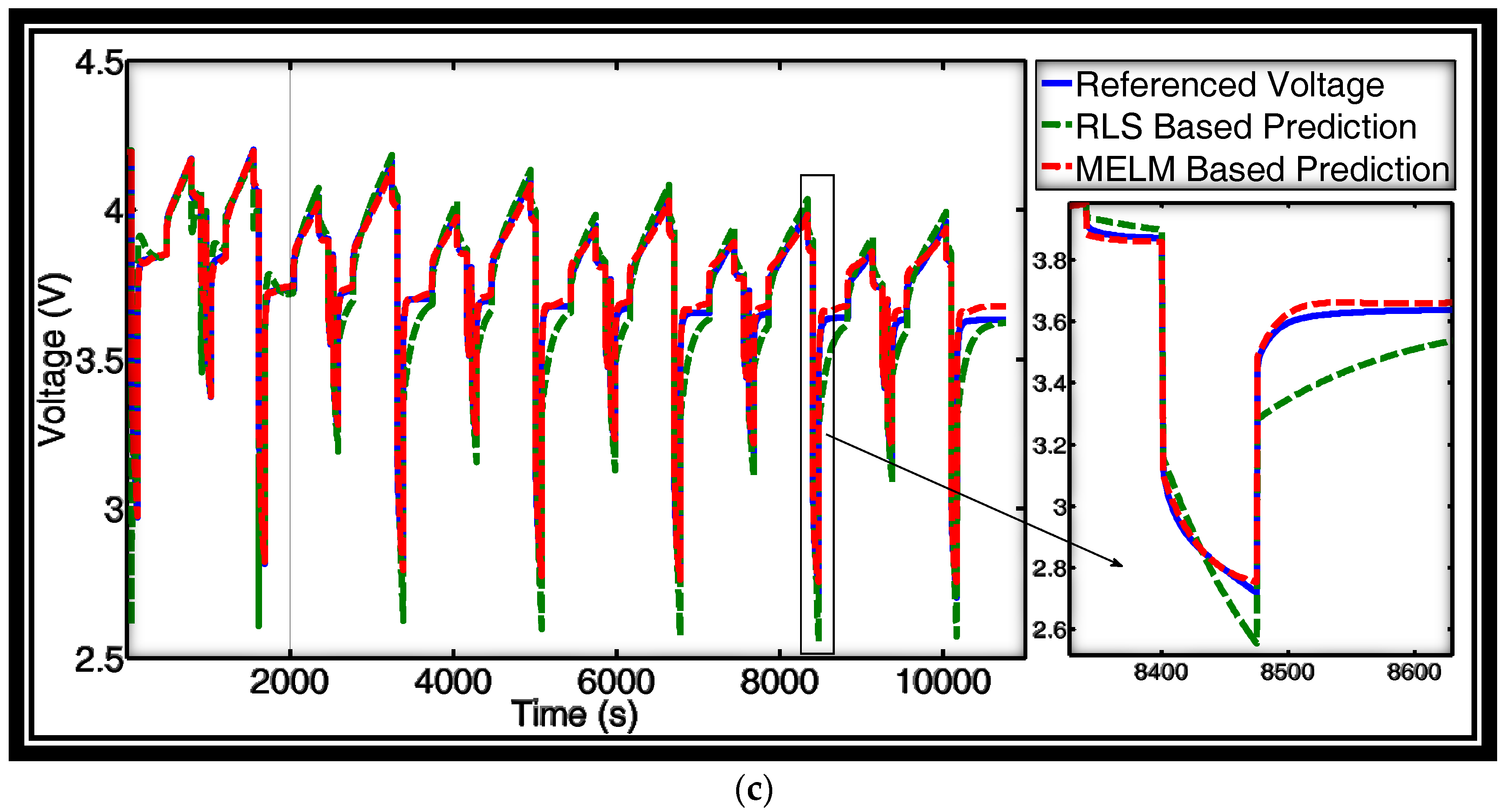
3.3.2. Voltage and Power Prediction
The results of the prediction of the battery’s voltage are provided in Figure 9. We also used an RLS-based method to predict the comparison of the algorithms. In the RLS-based prediction, the model parameters (R0, Cp, Rp) are identified following [39], the OCV and battery capacity at different temperatures are obtained from Figure 6 and Table 5, and the future temperatures are obtained using the results of the RLS method provided in Section 3.3.1.
The model obtained using the proposed MELM method shows the accuracy of the long-term prediction compared with the RLS-based method. Although RLS provides a minimal variance solution to the parameter identification problem, the model under identification, i.e., the Thevenin model itself, is not very accurate, as stated in the introduction. However, with the proposed MELM method, this not-very-accurate Thevenin model is embedded into an SLFN structure, which significantly improves the ability to approximate more complex nonlinear systems.
In this paper, the transient power is calculated by multiplying the voltage and current, and the root mean square error (RMSE) of the overall power prediction error of the three loads is listed in Table 6. The prediction result of the MELM method is indeed more accurate than using one model, even if this model has the same structure as MELM models and its parameters are calculated in an optimal fashion. It should also be noted that the proposed method can be transformed into a conventional SOP prediction by selecting the future load as a 10 s current pulse.
4. Conclusions
The prediction of a battery’s SOP usually covers a relatively short period of time (e.g., 10 s or 30 s). To provide effective long-term prediction, a MELM-based method is proposed to calculate the battery future surface temperature, voltage, and power. The original contributions in the proposed method are:
- The influence of both ambient temperature and temperature caused by Joule heat are considered.
- The influence of the SOC changing is considered for more accurate long-term prediction.
- The generalization performance of SLFN improves by using models to replace active functions.
- MELM provides an alternative way to identify systems with complex structures using only the least squares method, which can be calculated both offline and online.
- Power prediction accuracy does not rely on the accuracy of state estimation such as SOC.
Acknowledgments
We would like to thank Kaori Lkegaya for helping to correct the language problems. We would like to thank Yongxiao Xia and Zhenwei He for their assistance with the experiment. We would also like to acknowledge the financial support of the National Natural Science Foundation of China (61433005) and Guangdong scientific and technological project (2017B010120002).
Author Contributions
This research article has five authors. Xiaopeng Tang proposed the idea and wrote the paper. He also attended the conference and presented the original conference version of this paper in Sweden. Ke Yao and Furong Gao provided the experimental platform; Boyang Liu helped to correct the paper; Wengui Hu helped to do the experiments and collect the data; Furong Gao, the corresponding author, corrected the paper and is responsible for the paper.
Conflicts of Interest
The authors declare no conflict of interest.
References
- Lim, K.; Bastawrous, H.A.; Duong, V.-H.; See, K.W.; Zhang, P.; Dou, S.X. Fading Kalman filter-based real-time state of charge estimation in LiFePO 4 battery-powered electric vehicles. Appl. Energy 2016, 169, 40–48. [Google Scholar] [CrossRef]
- Xiong, R.; Zhang, Y.; He, H.; Zhou, X.; Pecht, M.G. A double-scale, particle-filtering, energy state prediction algorithm for lithium-ion batteries. IEEE Trans. Ind. Electron. 2017, PP, 1. [Google Scholar] [CrossRef]
- Xiong, R.; Cao, J.; Yu, Q. Reinforcement learning-based real-time power management for hybrid energy storage system in the plug-in hybrid electric vehicle. Appl. Energy 2018, 211, 538–548. [Google Scholar] [CrossRef]
- Thackeray, M.M.; Wolverton, C.; Isaacs, E.D. Electrical energy storage for transportation—Approaching the limits of, and going beyond, lithium-ion batteries. Energy Environ. Sci. 2012, 5, 7854–7863. [Google Scholar] [CrossRef]
- Chen, C.; Xiong, R.; Shen, W. A lithium-ion battery-in-the-loop approach to test and validate multi-scale dual H infinity filters for state of charge and capacity estimation. IEEE Trans. Power Electron. 2018, PP, 1. [Google Scholar]
- Tang, X.; Liu, B.; Lv, Z.; Gao, F. Observer based battery SOC estimation: Using multi-gain-switching approach. Appl. Energy 2017, 204, 1275–1283. [Google Scholar] [CrossRef]
- Xiong, R.; Tian, J.; Mu, H.; Wang, C. A systematic model-based degradation behavior recognition and health monitoring method for lithium-ion batteries. Appl. Energy 2017, 207, 372–383. [Google Scholar] [CrossRef]
- Wik, T.; Fridholm, B.; Kuusisto, H. Implementation and robustness of an analytically based battery state of power. J. Power Sources 2015, 287, 448–457. [Google Scholar] [CrossRef]
- Rahman, M.; Anwar, S.; Izadian, A. Electrochemical Model-Based Condition Monitoring via Experimentally Identified Li-Ion Battery Model and HPPC. Energies 2017, 10, 1266. [Google Scholar] [CrossRef]
- Plett, G.L. High-performance battery-pack power estimation using a dynamic cell model. IEEE Trans. Veh. Technol. 2004, 53, 1586–1593. [Google Scholar] [CrossRef]
- Wang, Y.; Pan, R.; Liu, C.; Chen, Z.; Ling, Q. Power capability evaluation for lithium iron phosphate batteries based on multi-parameter constraints estimation. J. Power Sources 2018, 374, 12–23. [Google Scholar] [CrossRef]
- Yu, Q.; Xiong, R.; Lin, C.; Shen, W.; Deng, J. Lithium-ion Battery Parameters and State-of-Charge Joint Estimation Based on H infinity and Unscented Kalman Filters. IEEE Trans. Veh. Technol. 2017, 66, 8693–8701. [Google Scholar] [CrossRef]
- Zhang, C.; Wang, L.Y.; Li, X.; Chen, W.; Yin, G.G.; Jiang, J. Robust and Adaptive Estimation of State of Charge for Lithium-Ion Batteries. IEEE Trans. Ind. Electron. 2015, 62, 4948–4957. [Google Scholar] [CrossRef]
- Liu, G.; Ouyang, M.; Lu, L.; Li, J.; Hua, J. A highly accurate predictive-adaptive method for lithium-ion battery remaining discharge energy prediction in electric vehicle applications. Appl. Energy 2015, 149, 297–314. [Google Scholar] [CrossRef]
- Jiang, J.; Liu, S.; Ma, Z.; Wang, L.Y.; Wu, K. Butler-Volmer equation-based model and its implementation on state of power prediction of high-power lithium titanate batteries considering temperature effects. Energy 2016, 117, 58–72. [Google Scholar] [CrossRef]
- Hausmann, A.; Depcik, C. Expanding the Peukert equation for battery capacity modeling through inclusion of a temperature dependency. J. Power Sources 2013, 235, 148–158. [Google Scholar] [CrossRef]
- Sun, F.; Xiong, R.; He, H. Estimation of state-of-charge and state-of-power capability of lithium-ion battery considering varying health conditions. J. Power Sources 2014, 259, 166–176. [Google Scholar] [CrossRef]
- Xu, Z.; Gao, S.; Yang, S. LiFePO4 battery state of charge estimation based on the improved Thevenin equivalent circuit model and Kalman filtering. J. Renew. Sustain. Energy 2016, 8, 376–378. [Google Scholar] [CrossRef]
- Wang, Y.; Chen, Z.; Zhang, C. On-line remaining energy prediction: A case study in embedded battery management system. Appl. Energy 2016, 194, 688–695. [Google Scholar] [CrossRef]
- Dong, G.; Chen, Z.; Wei, J.; Zhang, C.; Wang, P. An online model-based method for state of energy estimation of lithium-ion batteries using dual filters. J. Power Sources 2016, 301, 277–286. [Google Scholar] [CrossRef]
- Wang, S.; Verbrugge, M.; Wang, J.S.; Liu, P. Power prediction from a battery state estimator that incorporates diffusion resistance. J. Power Sources 2012, 214, 399–406. [Google Scholar] [CrossRef]
- Lu, L.; Han, X.; Li, J.; Hua, J.; Ouyang, M. A review on the key issues for lithium-ion battery management in electric vehicles. J. Power Sources 2013, 226, 272–288. [Google Scholar] [CrossRef]
- Wang, Y.; Zhang, C.; Chen, Z. A method for state-of-charge estimation of LiFePO4 batteries at dynamic currents and temperatures using particle filter. J. Power Sources 2015, 279, 306–311. [Google Scholar] [CrossRef]
- Liu, X.; Chen, Z.; Zhang, C.; Wu, J. A novel temperature-compensated model for power Li-ion batteries with dual-particle-filter state of charge estimation. Appl. Energy 2014, 123, 263–272. [Google Scholar] [CrossRef]
- Wang, T.; Tseng, K.J.; Zhao, J.; Wei, Z. Thermal investigation of lithium-ion battery module with different cell arrangement structures and forced air-cooling strategies. Appl. Energy 2014, 134, 229–238. [Google Scholar] [CrossRef]
- Murashko, K.; Pyrhönen, J.; Laurila, L. Three-dimensional thermal model of a lithium ion battery for hybrid mobile working machines: Determination of the model parameters in a pouch cell. IEEE Trans. Energy Convers. 2013, 28, 335–343. [Google Scholar] [CrossRef]
- Tang, X.; Liu, B.; Gao, F. State of Charge Estimation of LiFePO4 Battery Based on a Gain-classifier Observer. Energy Procedia 2017, 105, 2071–2076. [Google Scholar] [CrossRef]
- Tang, X.; Liu, B.; Gao, F.; Lv, Z. State-of-Charge Estimation for Li-Ion Power Batteries Based on a Tuning Free Observer. Energies 2016, 9, 675. [Google Scholar] [CrossRef]
- Xiong, R.; Yu, Q.; Wang, L.Y.; Lin, C. A novel method to obtain the open circuit voltage for the state of charge of lithium ion batteries in electric vehicles by using H infinity filter. Appl. Energy 2017, 207, 346–353. [Google Scholar] [CrossRef]
- Tang, X.; Wang, Y.; Chen, Z. A method for state-of-charge estimation of LiFePO4 batteries based on a dual-circuit state observer. J. Power Sources 2015, 296, 23–29. [Google Scholar] [CrossRef]
- Xiong, R.; Cao, J.; Yu, Q.; He, H.; Sun, F. Critical Review on the Battery State of Charge Estimation Methods for Electric Vehicles. IEEE Access 2017. [Google Scholar] [CrossRef]
- Huang, G.-B.; Chen, L. Enhanced random search based incremental extreme learning machine. Neurocomputing 2008, 71, 3460–3468. [Google Scholar] [CrossRef]
- Huang, G.-B.; Wang, D.H.; Lan, Y. Extreme learning machines: A survey. Int. J. Mach. Learn. Cybern. 2011, 2, 107–122. [Google Scholar] [CrossRef]
- Rumerhart, D.; Hinton, G.; Williams, R. Learning representations by back-propagation errors. Nature 1986, 323, 533–536. [Google Scholar] [CrossRef]
- Xu, L.; Wang, J.; Chen, Q. Kalman filtering state of charge estimation for battery management system based on a stochastic fuzzy neural network battery model. Energy Convers. Manag. 2012, 53, 33–39. [Google Scholar] [CrossRef]
- Zou, C.; Manzie, C.; Nesic, D.; Kallapur, A.G. Multi-time-scale observer design for state-of-charge and state-of-health of a lithium-ion battery. J. Power Sources 2016, 335, 121–130. [Google Scholar] [CrossRef]
- Zou, C.; Manzie, C.; Nešić, D. A Framework for Simplification of PDE-Based Lithium-Ion Battery Models. IEEE Trans. Control Syst. Technol. 2016, 24, 1594–1609. [Google Scholar] [CrossRef]
- Chen, Z.; Xiong, R.; Cao, J.; Lund, H.; Kaiser, M.J. Particle swarm optimization-based optimal power management of plug-in hybrid electric vehicles considering uncertain driving conditions. Energy 2016, 96, 197–208. [Google Scholar] [CrossRef]
- Xiong, R.; Sun, F.; He, H.; Nguyen, T.D. A data-driven adaptive state of charge and power capability joint estimator of lithium-ion polymer battery used in electric vehicles. Energy 2013, 63, 295–308. [Google Scholar] [CrossRef]
Figure 1.
General structure of three-layer neural network.
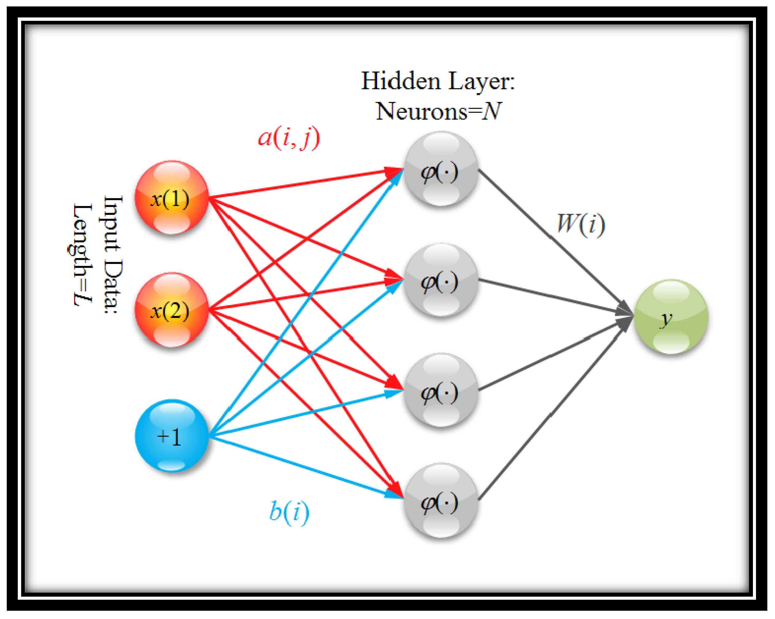
Figure 2.
Structure of the proposed model-based extreme learning machine.
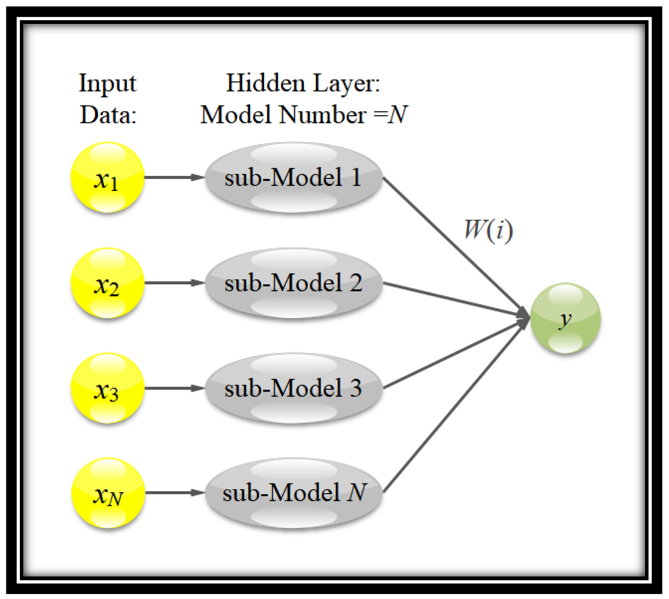
Figure 3.
Illustration of a parameter-distributed model using a battery surface temperature sensing example. The figure is a cross-sectional view of a cylinder battery.
Figure 3.
Illustration of a parameter-distributed model using a battery surface temperature sensing example. The figure is a cross-sectional view of a cylinder battery.
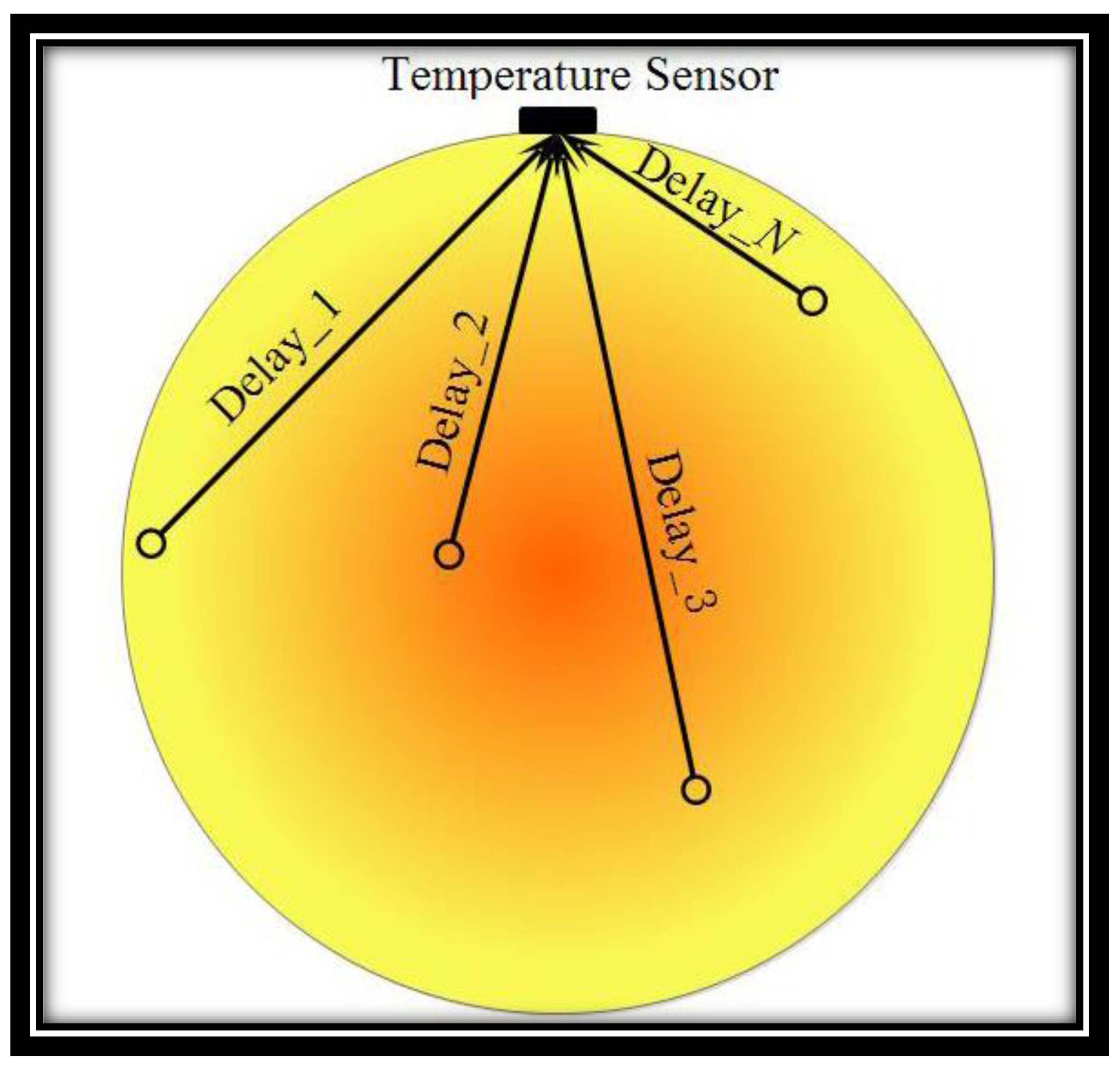
Figure 4.
Thevenin model.
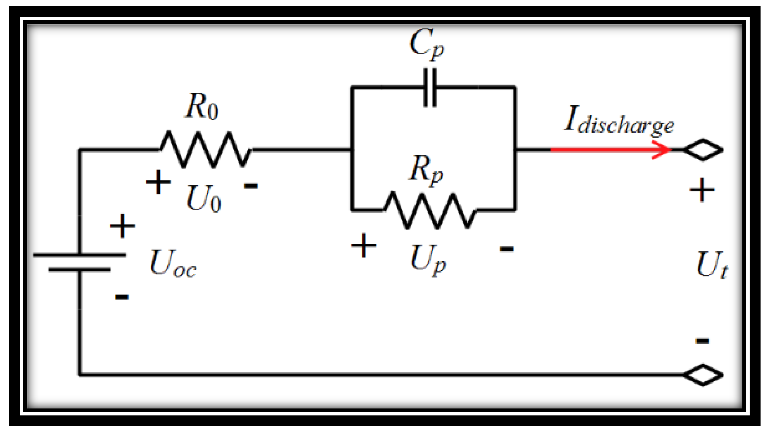
Figure 5.
Photo of experimental battery and devices.
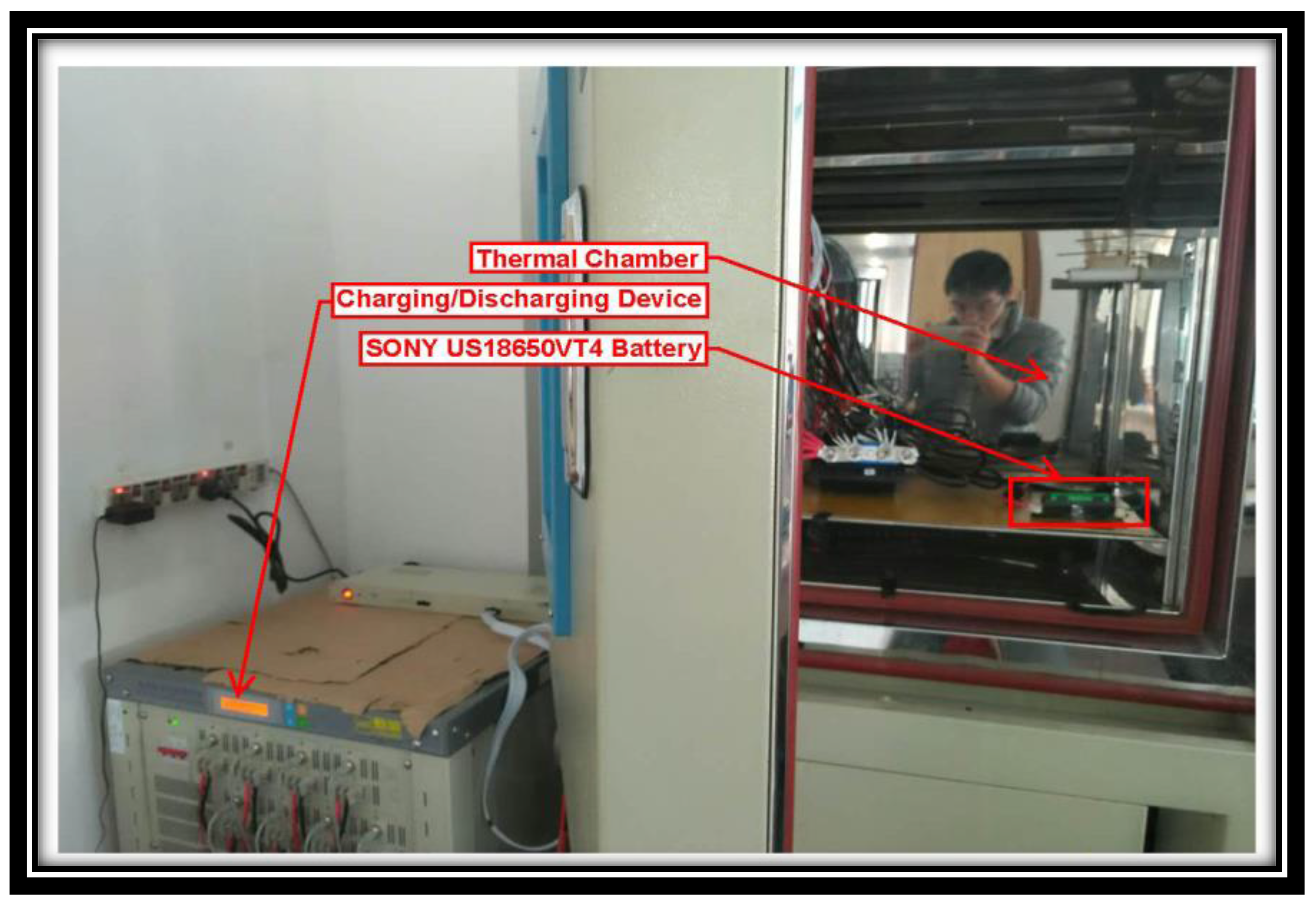
Figure 6.
Open circuit voltage–state of charge relationship at different temperatures.

Figure 7.
Load conditions and corresponding temperature response. (a) Ambient temperature 5 °C; (b) ambient temperature 25 °C; (c) ambient temperature 45 °C.
Figure 7.
Load conditions and corresponding temperature response. (a) Ambient temperature 5 °C; (b) ambient temperature 25 °C; (c) ambient temperature 45 °C.
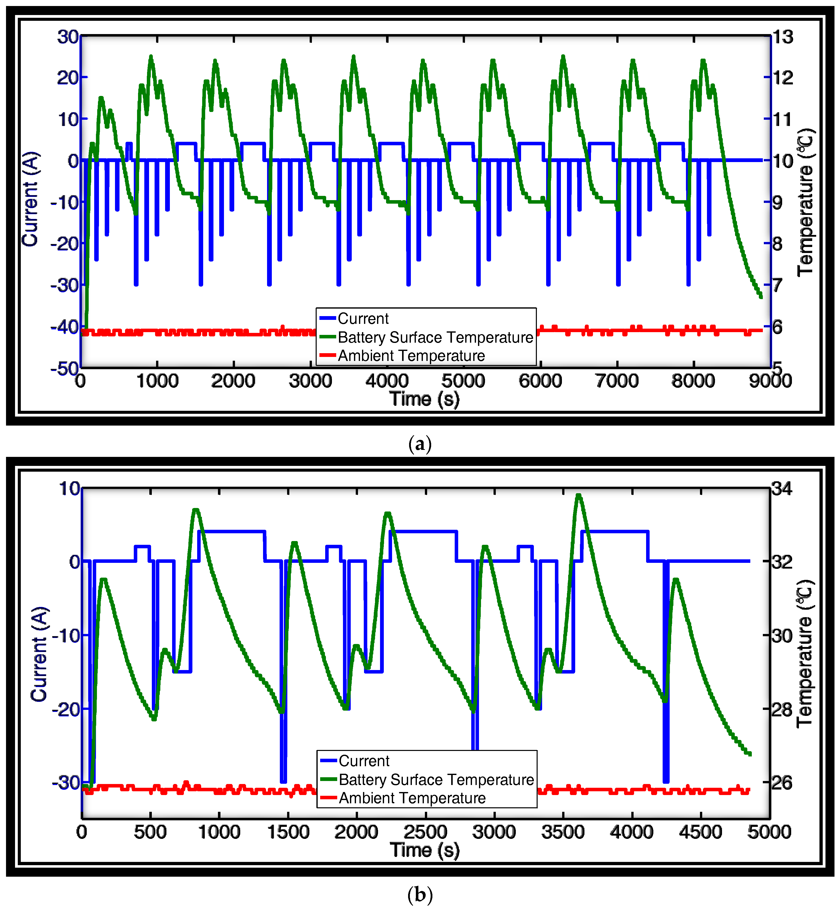

Figure 8.
Temperature prediction result of different methods. (a) Load (a) at 5 °C; (b) load (b) at 25 °C; (c) load (c) at 45 °C.
Figure 8.
Temperature prediction result of different methods. (a) Load (a) at 5 °C; (b) load (b) at 25 °C; (c) load (c) at 45 °C.

Figure 9.
Voltage prediction result of different methods. (a) Load (a) at 5 °C; (b) load (b) at 25 °C; (c) load (c) at 45 °C.
Figure 9.
Voltage prediction result of different methods. (a) Load (a) at 5 °C; (b) load (b) at 25 °C; (c) load (c) at 45 °C.


Table 1.
Online recursive least squares with forgetting factor.
| Step | Name | Details |
|---|---|---|
| 1 | Initialization | P = 105I, λ = 0.995, W = |
| 2 | Gain Calculation | K = P·hT/(λ + h·P·hT) |
| 3 | P Calculation | P = (I − K·h)·P/λ |
| 4 | W Calculation | W = W + K·(Y − h·W) |
| 5 | Loop | Loop to Step 2 |
Table 2.
Summary of the model-based extreme learning machine (MELM) procedure.
| Stages | Methods |
|---|---|
| Offline | 1. Randomly generate N temperature models; |
| 2. Randomly generate N equivalent circuit models; | |
| Online Training | 1. Use RLS to obtain weight matrix W1 for temperature models; |
| 2. Use RLS to obtain weight matrix W2 for equivalent circuit models; | |
| Future Prediction | 1. Design the current profile that should be predicted (e.g., a 10 s pulse, or some long lasting current profiles) |
| 2. Calculate the future temperature based on the future current load profile and W1 | |
| 3. Calculate the future terminal voltage based on the future current load profile, calculated temperature and W2. | |
| 4. Check whether the voltage and the temperature exceed the limits. |
Table 3.
Battery and device models.
| Battery Type: | Battery Capacity | Device Model |
|---|---|---|
| SONY US18650VTC4 | 2.10 Ah (Manufacturer Data) | Electronic Load: Sunway CT4008 W |
| 1.90 Ah (Experimental Data, 25 °C) | Thermal Chamber: Bole GDS150 |
Table 4.
Battery temperature model.
| Parameter | Suggested Value | Range |
|---|---|---|
| α | 0.99916 | (0.995, 0.9999) |
| β | 0.000067 | (0.00005, 0.001) |
| γ | 1 | (0.3, 3) |
| delay | 50 (s) | [0,100], integer |
Table 5.
Parameter selection of the Thevenin model.
| Parameter | Suggested Value at 25 °C * | Range | Suggested ci Value | Range |
|---|---|---|---|---|
| Cn | 1.90 Ah | (1.5, 2.15) Ah | 8.79 mAh/°C | (3, 18) mAh/°C |
| R0 | 0.0240 Ω | (0.005, 0.08) Ω | −0.97 mΩ/°C | (−2, −0.2) mΩ/°C |
| Rp | 0.0362 Ω | (0.005, 0.08) Ω | 0 mΩ/°C ** | (−1, 1) mΩ/°C |
| Cp | 2445 F | (500, 10,000) F | 5 F/°C | (−0.5, 12) F/°C |
| HY | 0 mV | (−10, 10) mV | 0 mV/°C | (−1, 1) mV/°C |
| Initial SOC | Vref = look up table value | Vref ± 10% | - | - |
| Initial Up | 0 mV | - | - | - |
* The value is obtained using data in the full SOC range. ** No obvious relationship between Rp and temperature has been observed.
Table 6.
Root mean square error (RMSE) of power prediction.
| Temperature (°C) | RLS Error (W) | MELM Error (W) |
|---|---|---|
| 05 | 0.372 | 0.172 |
| 25 | 0.376 | 0.217 |
| 45 | 0.552 | 0.139 |
© 2018 by the authors. Licensee MDPI, Basel, Switzerland. This article is an open access article distributed under the terms and conditions of the Creative Commons Attribution (CC BY) license (http://creativecommons.org/licenses/by/4.0/).
Share and Cite
MDPI and ACS Style
Tang, X.; Yao, K.; Liu, B.; Hu, W.; Gao, F. Long-Term Battery Voltage, Power, and Surface Temperature Prediction Using a Model-Based Extreme Learning Machine. Energies 2018, 11, 86. https://doi.org/10.3390/en11010086
AMA Style
Tang X, Yao K, Liu B, Hu W, Gao F. Long-Term Battery Voltage, Power, and Surface Temperature Prediction Using a Model-Based Extreme Learning Machine. Energies. 2018; 11(1):86. https://doi.org/10.3390/en11010086
Chicago/Turabian StyleTang, Xiaopeng, Ke Yao, Boyang Liu, Wengui Hu, and Furong Gao. 2018. "Long-Term Battery Voltage, Power, and Surface Temperature Prediction Using a Model-Based Extreme Learning Machine" Energies 11, no. 1: 86. https://doi.org/10.3390/en11010086
Note that from the first issue of 2016, this journal uses article numbers instead of page numbers. See further details here.