Improved Krill Herd Algorithm with Novel Constraint Handling Method for Solving Optimal Power Flow Problems

Abstract
:1. Introduction
- An improved krill herd algorithm is proposed, namely IKHA, which introduces the onlooker search mechanism to reduce the probability of falling into local optimum. Moreover, the parameter values of the proposed algorithm including inertia weight ω and step-length scale factor Ct are varied according to the iteration of evolutionary process.
- A novel constraint handling method, which contains two parts of control variable constraint and state variable constraint, is proposed to guide the individual to the feasible space and ensure the optimal solutions satisfy the security constraints, especially in larger systems.
- The OPF problem is successfully implemented on standard IEEE 30 bus, IEEE 57 bus and IEEE 118 bus systems to solve 10 different cases by using the proposed method.
2. OPF Problem Formulation
2.1. Control Variable
2.2. State Variable
2.3. Equality Constraint
2.4. Inequality Constraint
- Generator constraints:
- Transformer constraints:
- Shunt reactive compensator constraints:
- Security constraints:
3. Improved Krill Herd Algorithm (IKHA)
3.1. Brief on Krill Herd Algorithm (KHA)
- Movement induced by other krill individuals
- Foraging motion
- Random diffusion
3.1.1. Movement Induced by Other Krill Individuals
3.1.2. Foraging Motion
3.1.3. Random Diffusion
3.1.4. Position Update
3.1.5. Genetic Operators
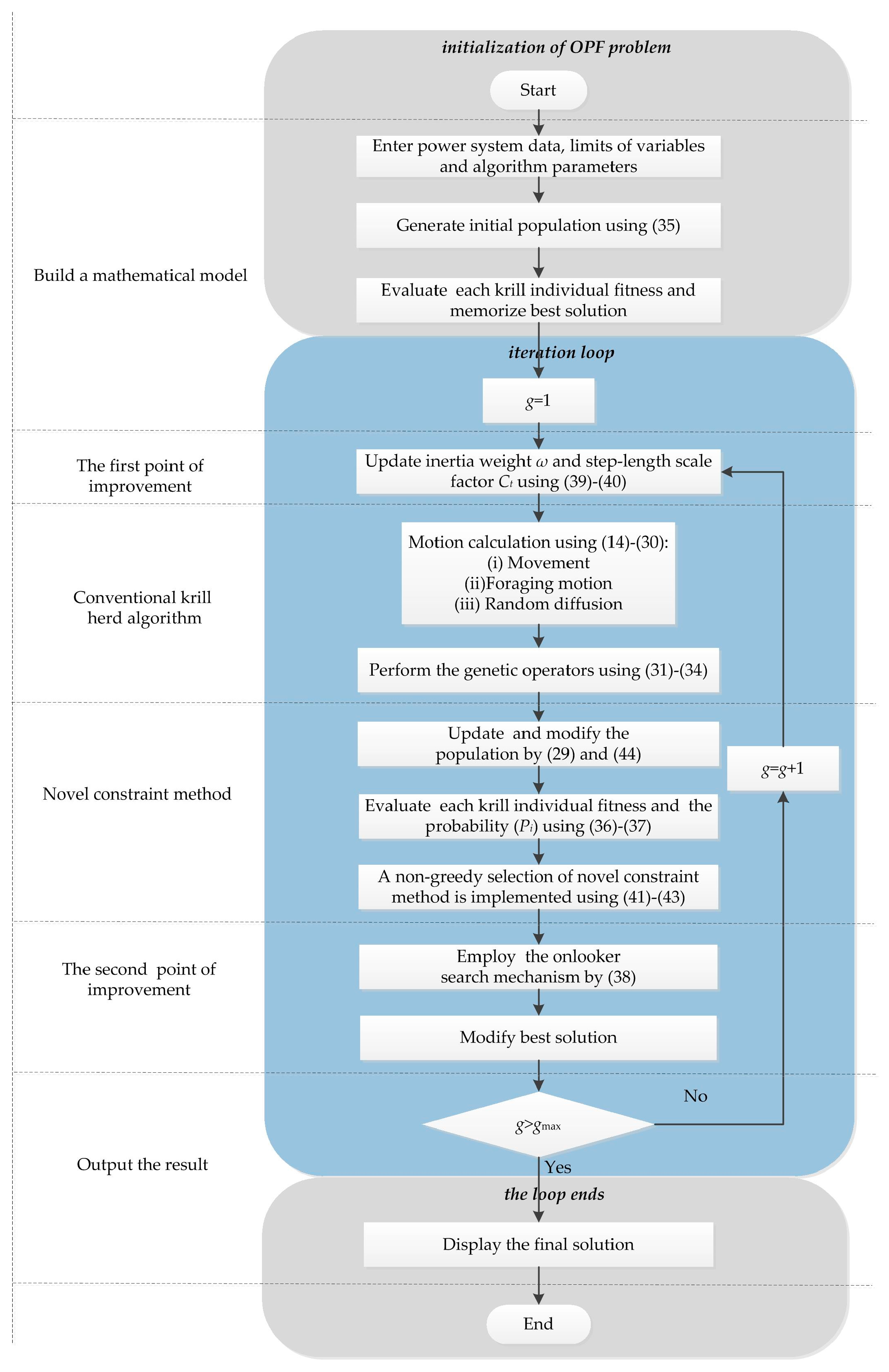
3.1.6. The Process of Krill Herd Algorithm
- Step 1:
- Initialization: The algorithm parameters, the power system data, limits of variables.
- Step 2:
- The generation of initial population: The individual is randomly generated in the search space of the optimization problem. Random values are assigned to each D-dimensional individual according to:where Xj,min and Xj,max represent the lower and upper bounds of the jth decision variable, NP is the population size, rand5 is uniformly distributed random variable between 0 and 1.
- Step 3:
- Fitness evaluation: Evaluate each krill individual according to its position and memorise the global best solution.
- Step 4:
- Motion calculation:
- Movement induced by other krill individuals
- Foraging motion
- Random diffusion
- Step 5:
- Perform the genetic operators including crossover and mutation.
- Step 6:
- Update the population and repeat the Step 3.
- Step 7:
- Stop and display the final solution if the stop criteria is reached, else go back to Step 4.
3.2. Onlooker Search Mechanism
3.3. Parameter Improvement
3.4. Implementation of IKHA Algorithm
4. Novel Constraint Handling Method
4.1. State Variable Constraint
4.2. Control Variable Constraint
5. Application and Simulation Results
5.1. IEEE 30 Bus System
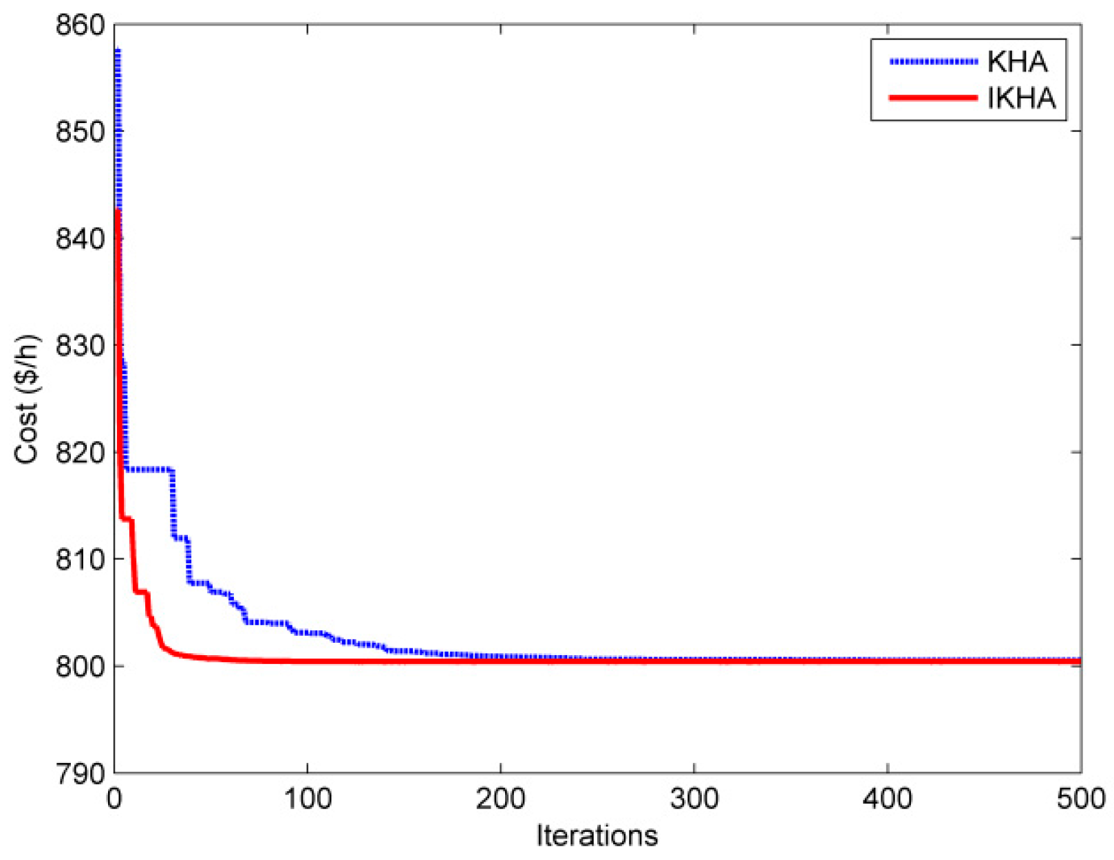
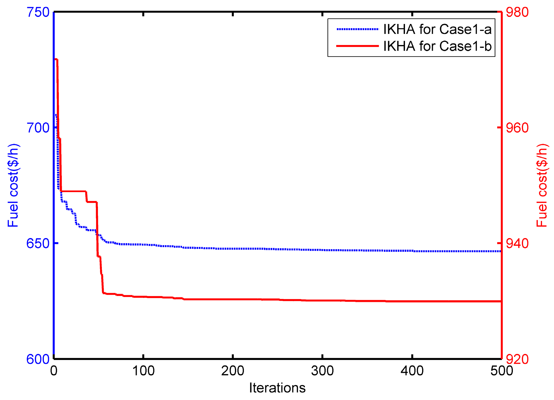
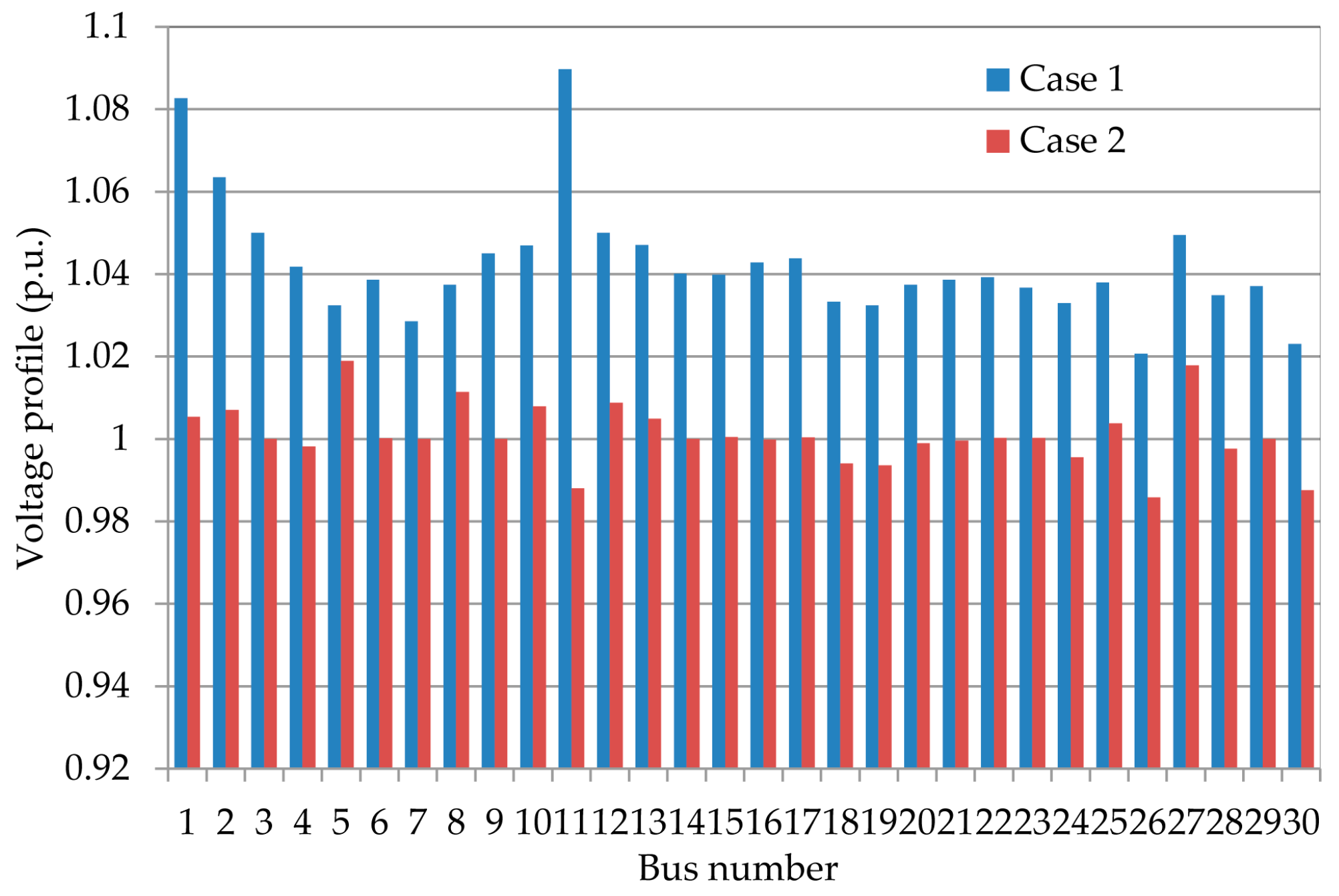
5.1.1. Case 1: Minimization of Quadratic Fuel Cost Function
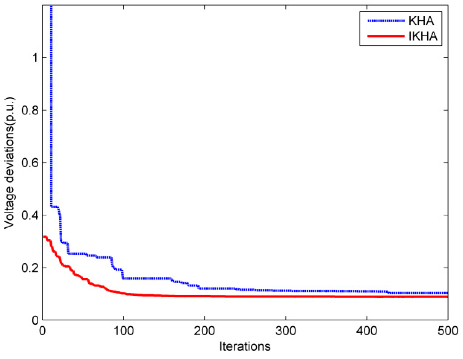
5.1.2. Case 2: Minimization of Voltage Magnitude Deviation
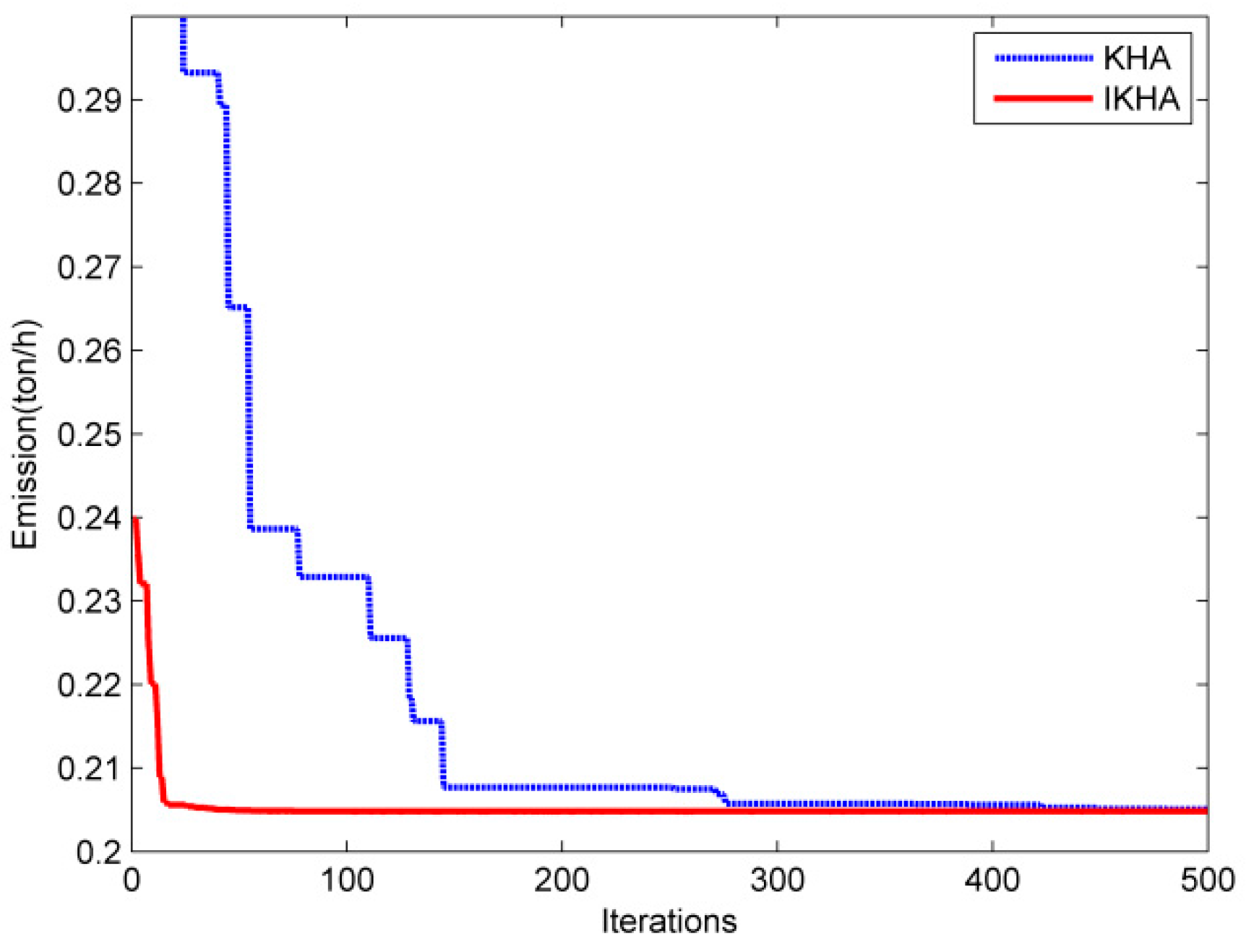
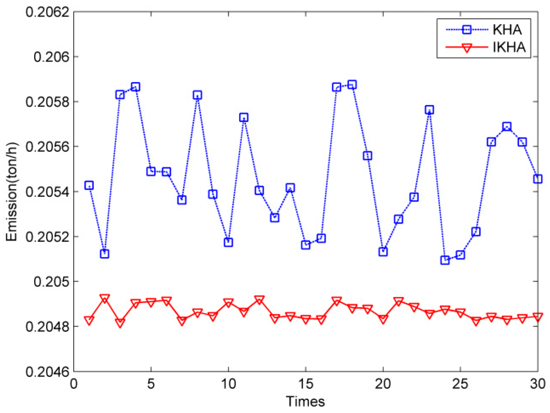
5.1.3. Case 3: Minimization of Fuel Cost Emission
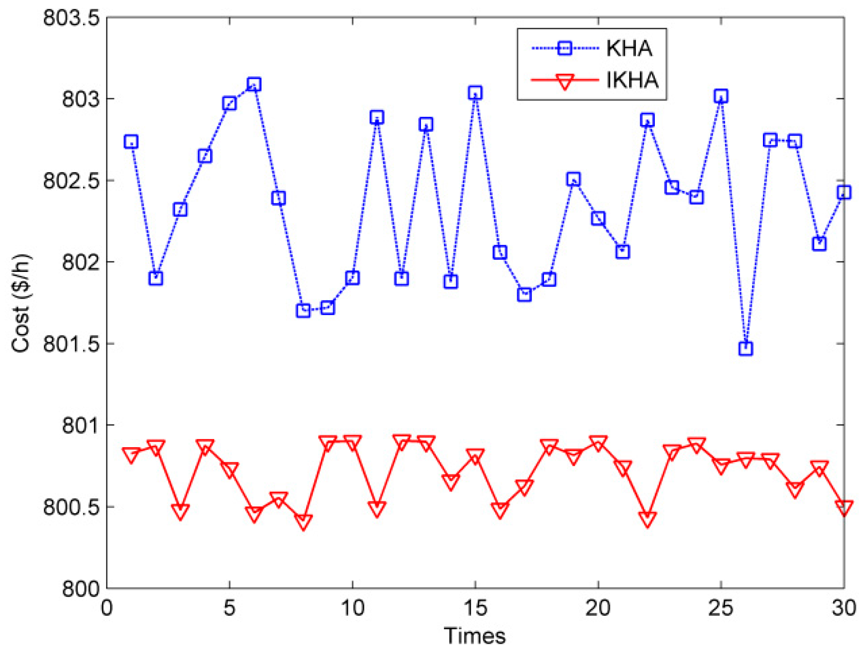
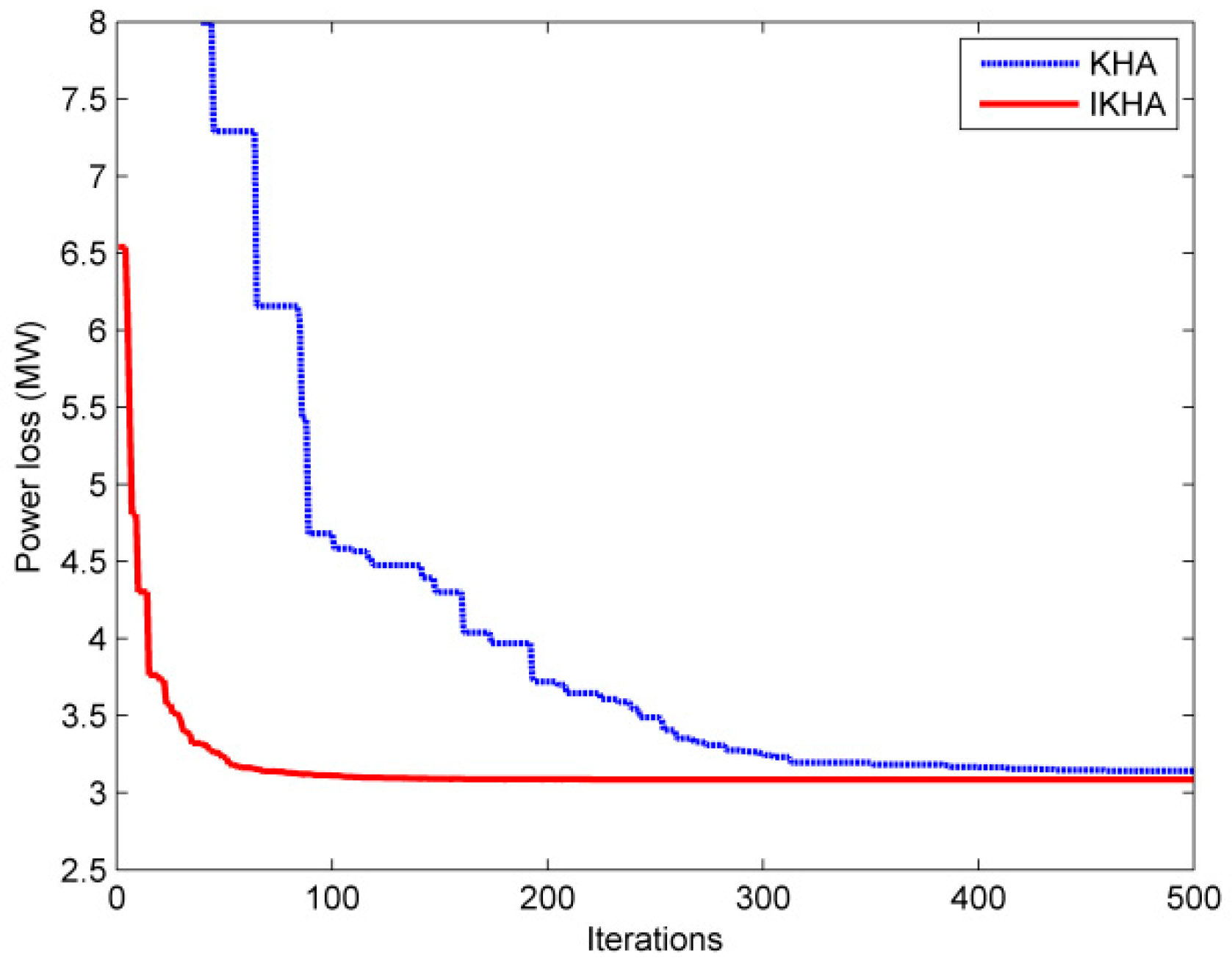
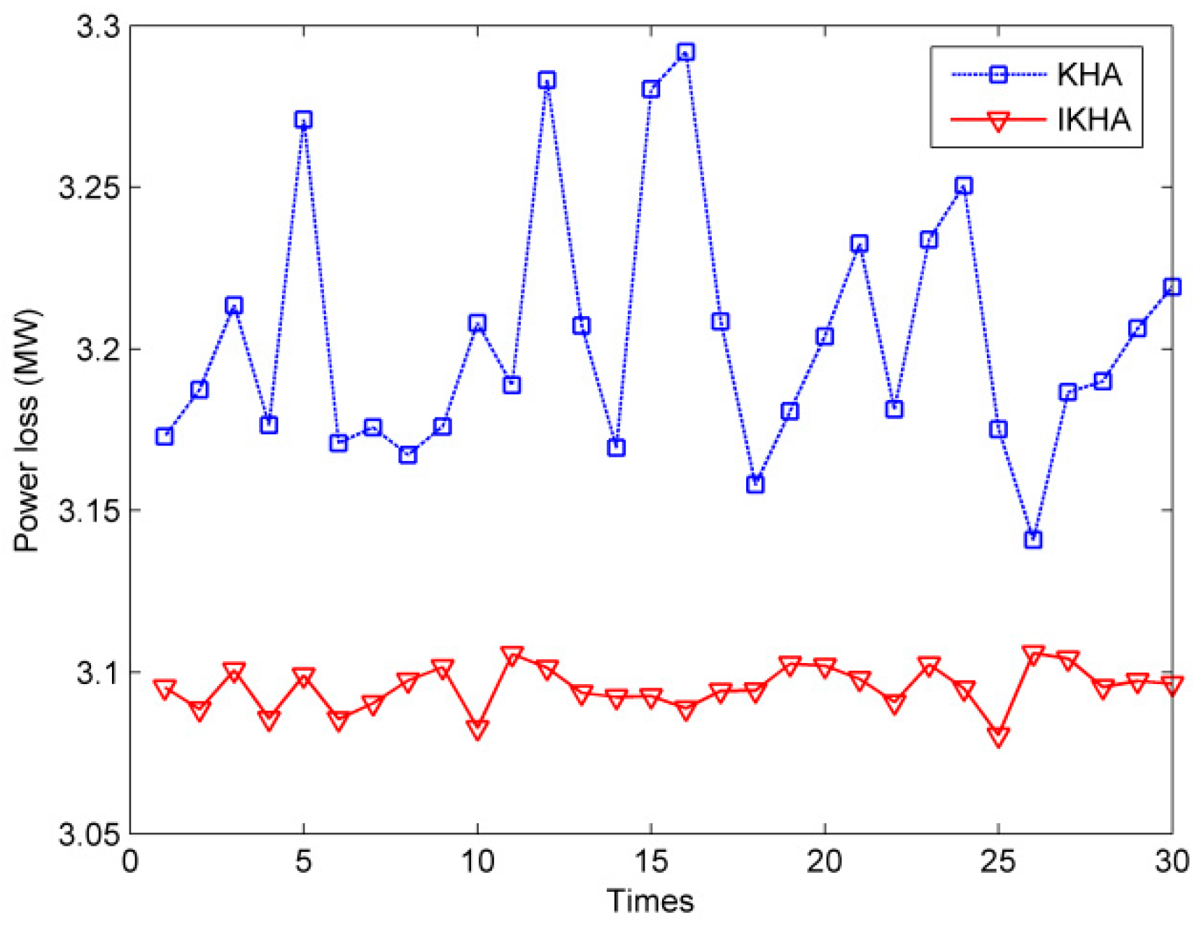
5.1.4. Case 4: Minimization of Transmission Real Power Losses
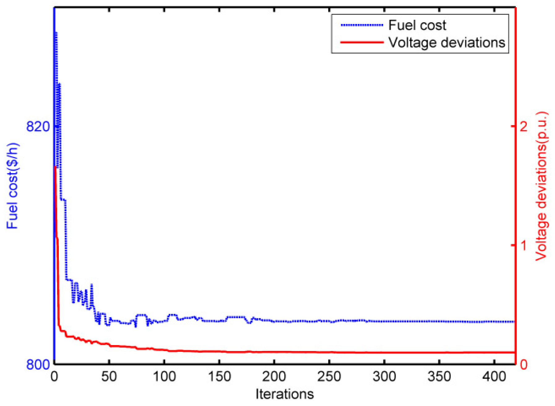
5.1.5. Case 5: Minimization of Quadratic Cost and Voltage Magnitude Deviation
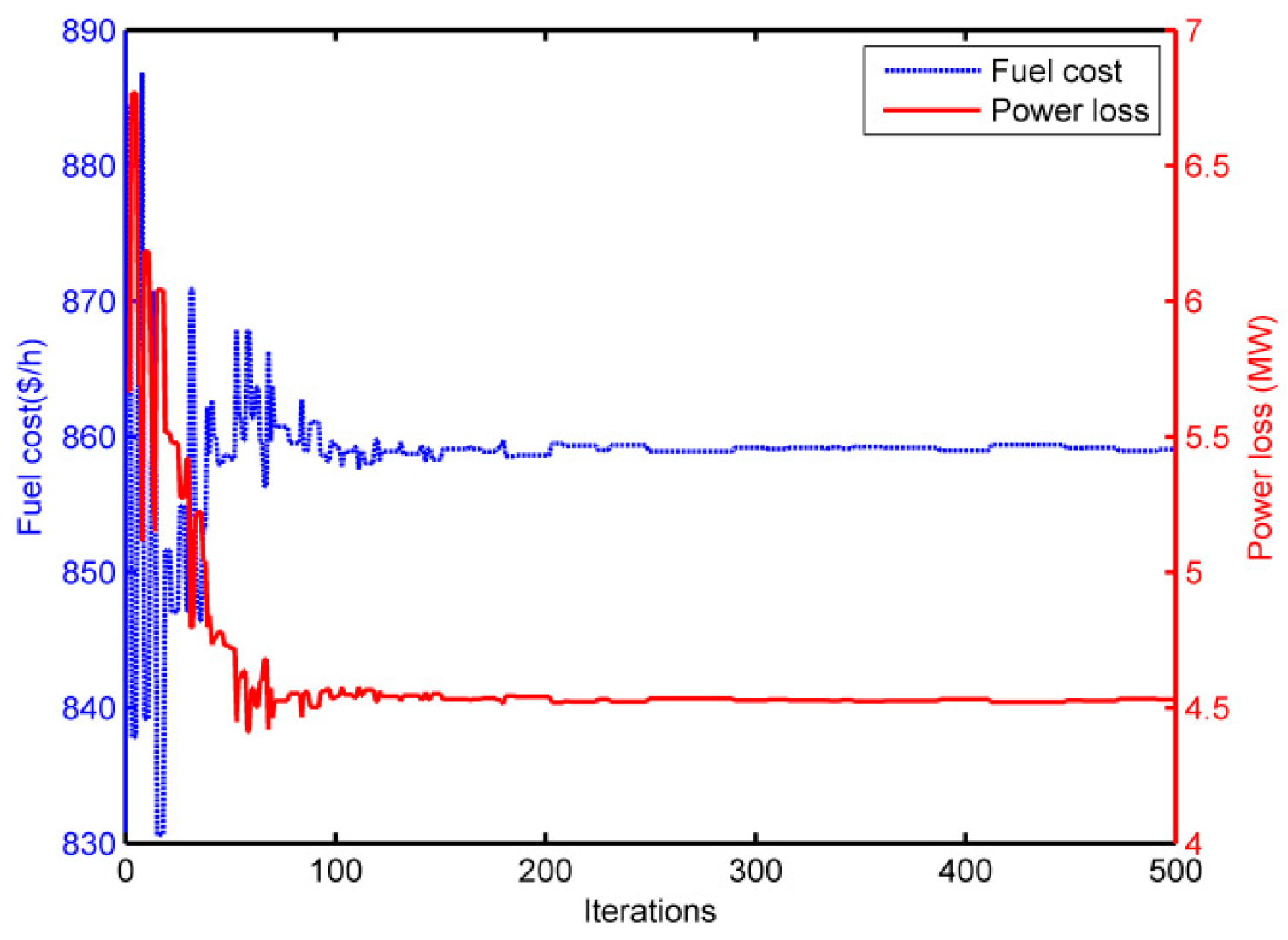
5.1.6. Case 6: Minimization of Quadratic Cost and Transmission Real Power Losses
5.2. IEEE 57 Bus System
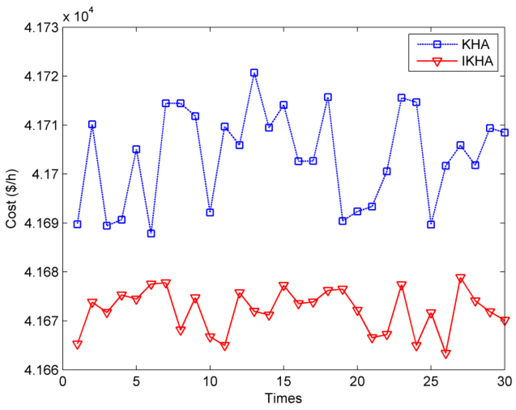
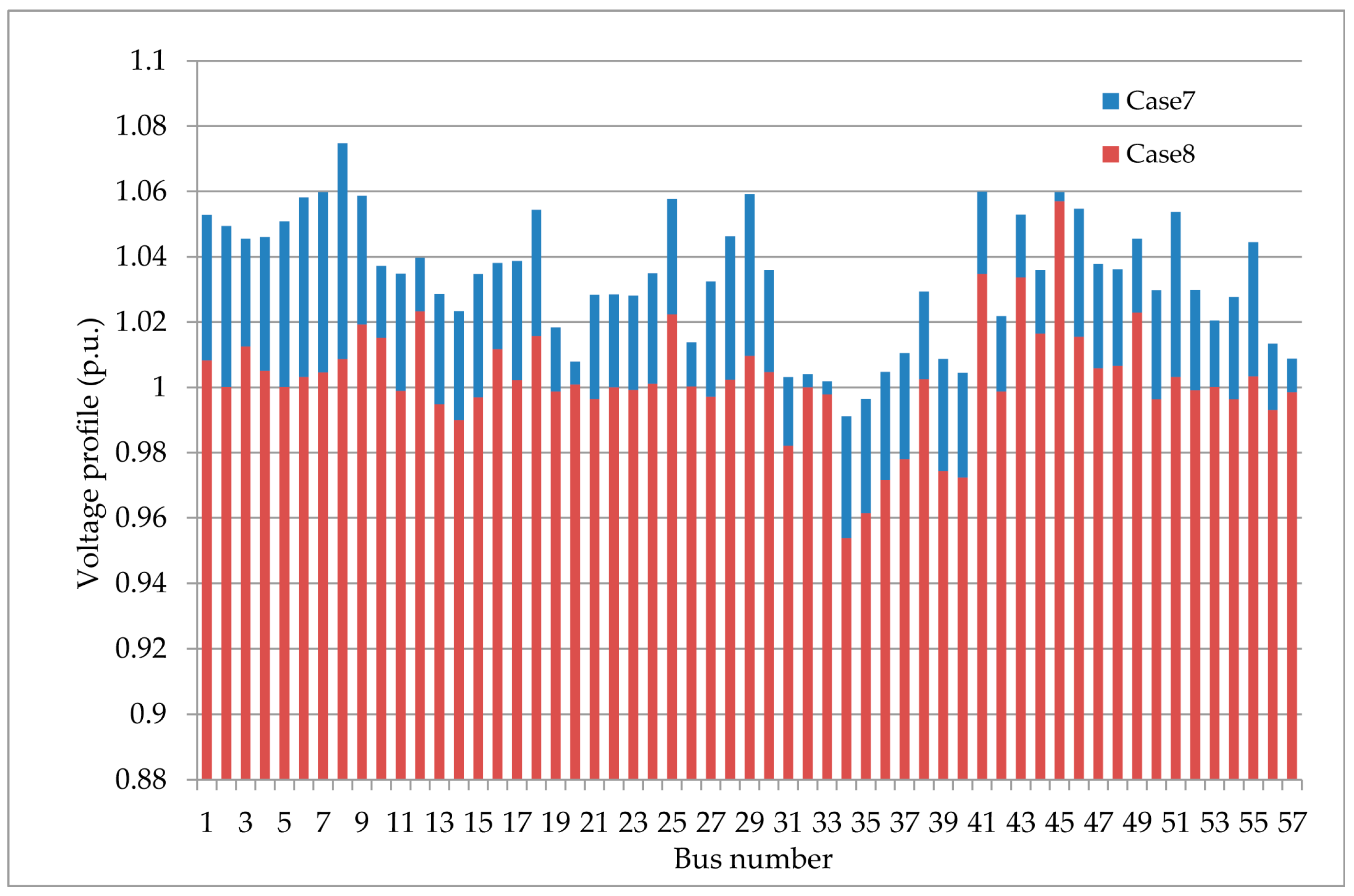
5.2.1. Case 7: Minimization of Quadratic Fuel Cost Function
5.2.2. Case 8: Minimization of Voltage Magnitude Deviation
5.2.3. Case 9: Minimization of Quadratic Cost and Voltage Magnitude Deviation
5.3. IEEE 118 Bus System
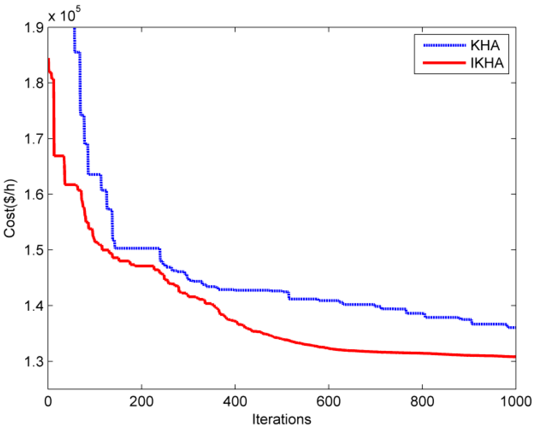
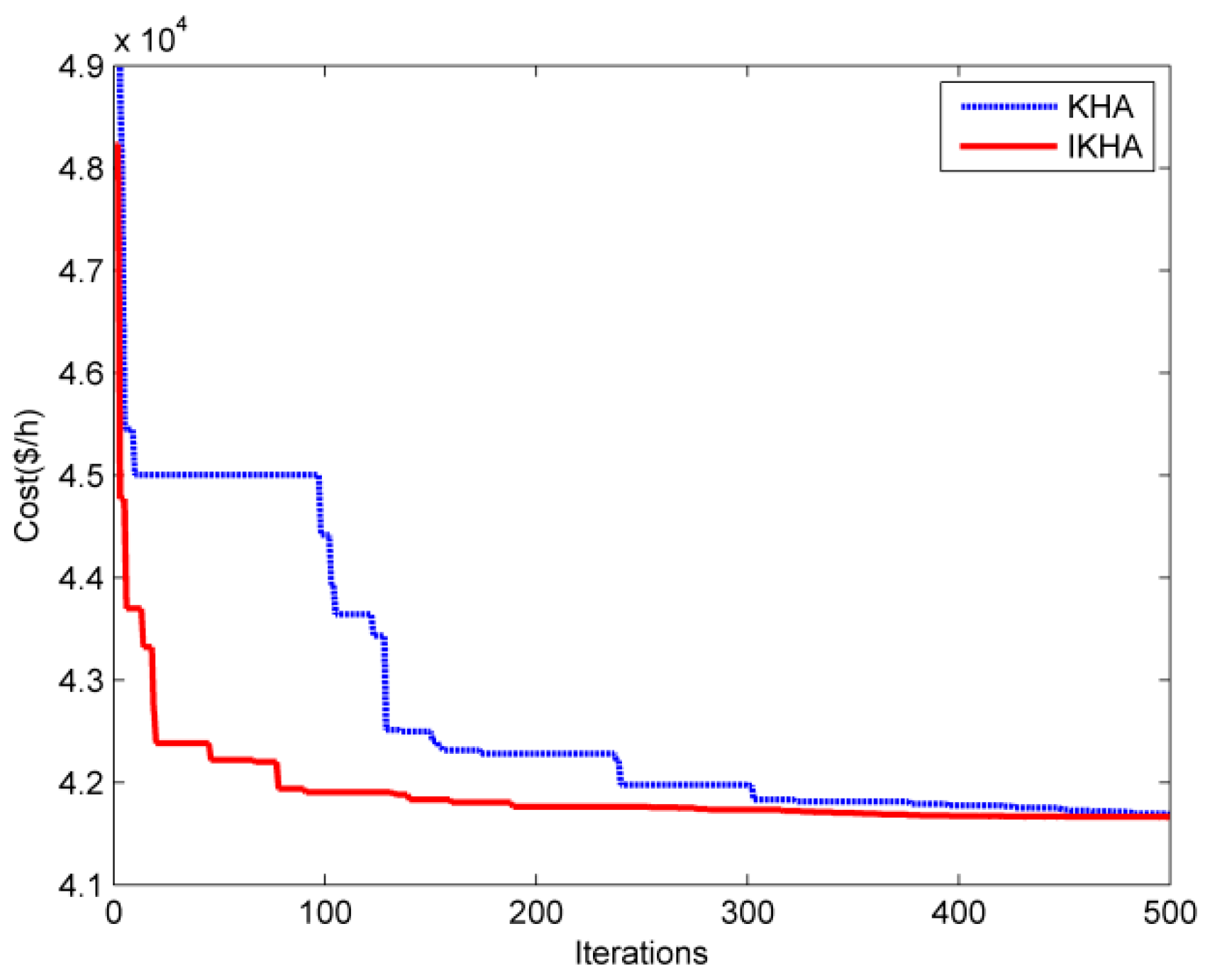
Case 10: Minimization of Quadratic Fuel Cost Function
6. Conclusions
Acknowledgments
Author Contributions
Conflicts of Interest
References
- Daryani, N.; Hagh, M.T.; Teimourzadeh, S. Adaptive Group Search Optimization Algorithm for Multi-Objective Optimal Power Flow Problem. Appl. Soft Comput. 2016, 38, 1012–1024. [Google Scholar] [CrossRef]
- Sanseverino, E.R.; di Silvestre, M.L.; Badalamenti, R.; Nguyen, N.Q.; Guerrero, J.M.; Meng, L. Optimal Power Flow in Islanded Microgrids Using a Simple Distributed Algorithm. Energies 2015, 8, 11493–11514. [Google Scholar] [CrossRef] [Green Version]
- Capitanescu, F.; Glavic, M.; Ernst, D.; Wehenkel, L. Interior-point based algorithms for the solution of optimal power flow problems. Electr. Power Syst. Res. 2007, 77, 508–817. [Google Scholar] [CrossRef]
- Mota-Palomino, B.; Quintana, V.H. Sparse Reactive Power Scheduling by a Penalty Function—Linear Programming Technique. IEEE Trans. Power Syst. 1986, 1, 31–39. [Google Scholar] [CrossRef]
- Shoults, R.; Sun, D. Optimal Power Flow Based Upon P-Q Decomposition. IEEE Trans. Power Appar. Syst. 1982, PAS-101, 397–405. [Google Scholar] [CrossRef]
- Carpentier, J. Contribution a l’Etude du Dispatching Economique. Bulletin de la Societe Francaise des Electriciens 1962, 3, 431–474. [Google Scholar]
- Oliva, D.; Ewees, A.A.; Aziz, M.A.E.; Hassanien, A.E.; Cisneros, M.P. A Chaotic Improved Artificial Bee Colony for Parameter Estimation of Photovoltaic Cells. Energies 2017, 10, 865. [Google Scholar] [CrossRef]
- Khaled, U.; Eltamaly, A.; Beroual, A. Optimal Power Flow Using Particle Swarm Optimization of Renewable Hybrid Distributed Generation. Energies 2017, 10, 1013. [Google Scholar] [CrossRef]
- Abaci, K.; Yamacli, V. Differential search algorithm for solving multi-objective optimal power flow problem. Electr. Power Energy Syst. 2016, 79, 1–10. [Google Scholar] [CrossRef]
- Zhao, Z.; Yang, J.; Hu, Z.; Che, H. A differential evolution algorithm with self-adaptive strategy and control parameters based on symmetric Latin hypercube design for unconstrained optimization problems. Eur. J. Oper. Res. 2016, 250, 30–45. [Google Scholar] [CrossRef]
- Chen, G.; Liu, L.; Zhang, Z.; Huang, S. Optimal reactive power dispatch by improved GSA-based algorithm with the novel strategies to handle constraints. Appl. Soft Comput. 2017, 50, 58–70. [Google Scholar] [CrossRef]
- Bouchekara, H.R.E.H.; Chaib, A.E.; Abido, M.A.; El-Sehiemy, R.A. Optimal power flow using an Improved Colliding Bodies Optimizationalgorithm. Appl. Soft Comput. 2016, 42, 119–131. [Google Scholar] [CrossRef]
- Singh, R.P.; Mukherjee, V.; Ghoshal, S.P. Particle swarm optimization with an aging leader and challengers algorithm for the solution of optimal power flow problem. Appl. Soft Comput. 2016, 40, 161–177. [Google Scholar] [CrossRef]
- Capitanescu, F. Critical review of recent advances and further developments needed in AC optimal power flow. Electr. Power Syst. Res. 2016, 136, 57–68. [Google Scholar] [CrossRef]
- Gandomi, A.H.; Alavi, A.H. Krill herd: A new bio-inspired optimization algorithm. Commun. Nonlinear Sci. Numer. Simul. 2012, 12, 4831–4845. [Google Scholar] [CrossRef]
- Mukherjee, A.; Mukherjee, V. Chaos embedded krill herd algorithm for optimal VAR dispatch problem of power system. Electr. Power Energy Syst. 2016, 82, 37–48. [Google Scholar] [CrossRef]
- Bulatović, R.R.; Miodragović, G.; Bošković, M.S. Modified Krill Herd (MKH) algorithm and its application in dimensional synthesis of a four-bar linkage. Mech. Mach. Theory 2016, 95, 1–21. [Google Scholar] [CrossRef]
- Sultana, S.; Roy, P.K. Oppositional krill herd algorithm for optimal location of capacitor with reconfiguration in radial distribution system. Electr. Power Energy Syst. 2016, 74, 78–90. [Google Scholar] [CrossRef]
- Wang, G.; Deb, S.; Gandomi, A.H.; Abaci, K. Opposition-based krill herd algorithm with Cauchy mutation and position clamping. Neurocomputing 2016, 177, 147–157. [Google Scholar] [CrossRef]
- Wang, H.; Wang, W.; Sun, H.; Cui, Z.; Rahnamayan, S.; Zeng, S. A new cuckoo search algorithm with hybrid strategies for flow shop scheduling problems. Soft Comput. 2017, 21, 4297–4307. [Google Scholar] [CrossRef]
- Cui, L.; Li, G.; Zhua, Z.; Lin, Q.; Wen, Z. A novel artificial bee colony algorithm with an adaptive population size for numerical function optimization. Inf. Sci. 2017, 414, 53–67. [Google Scholar] [CrossRef]
- Mohamed, A.A.; Mohamed, Y.S.; El-Gaafary, A.A.M. Optimal power flow using moth swarm algorithm. Electr. Power Syst. Res. 2017, 142, 190–206. [Google Scholar] [CrossRef]
- Ghasemi, M.; Ghavidel, S.; Gitizadeh, M.; Akbari, E. An improved teaching–learning-based optimization algorithm using Lévy mutation strategy for non-smooth optimal power flow. Electr. Power Energy Syst. 2015, 65, 375–384. [Google Scholar] [CrossRef]
- Roy, R.; Jadhav, H.T. Optimal power flow solution of power system incorporating stochastic wind power using Gbest guided artificial bee colony algorithm. Electr. Power Energy Syst. 2015, 64, 562–578. [Google Scholar] [CrossRef]
- Xia, X. Particle Swarm Optimization Method Based on Chaotic Local Search and Roulette Wheel Mechanism. Phys. Procedia 2012, 24, 269–275. [Google Scholar] [CrossRef]
- Singh, M.; Dhillon, J.S. Multiobjective thermal power dispatch using opposition-based greedy heuristic search. Electr. Power Energy Syst. 2016, 82, 339–353. [Google Scholar] [CrossRef]
- Alsac, O.; Stott, B. Optimal Load Flow with Steady-State Security. IEEE Trans. Power Appar. Syst. 1974, 93, 745–751. [Google Scholar] [CrossRef]
- Reddy, S.S.; Bijwe, P.R. Efficiency improvements in meta-heuristic algorithms to solve the optimal power flow problem. Electr. Power Energy Syst. 2016, 82, 288–302. [Google Scholar] [CrossRef]
- Radosavljević, R.; Klimenta, D. Optimal Power Flow Using a Hybrid Optimization Algorithm of Particle Swarm Optimization and Gravitational Search Algorithm. Electr. Power Compon. Syst. 2015, 17, 1958–1970. [Google Scholar] [CrossRef]
- Niknam, T.; Narimani, M.R. A modified shuffle frog leaping algorithm for multi-objective optimal power flow. Energy 2011, 36, 6420–6432. [Google Scholar] [CrossRef]
- Adaryani, M.R.; Karami, A. Artificial bee colony algorithm for solving multi-objective optimal power flow problem. Electr. Power Energy Syst. 2013, 53, 219–230. [Google Scholar] [CrossRef]
- Ghasemi, M.; Ghavidel, S.; Ghanbarian, M.M.; Gitizadeh, M. Multi-objective optimal electric power planning in the power system using Gaussian bare-bones imperialist competitive algorithm. Inf. Sci. 2015, 294, 286–304. [Google Scholar] [CrossRef]
- Warid, W.; Hizam, H.; Mariun, N.; Abdul-Wahab, N.I. Optimal Power Flow Using the Jaya Algorithm. Energies 2016, 9, 678. [Google Scholar] [CrossRef]
- Kumar, A.R.; Premalatha, L. Optimal power flow for a deregulated power system using adaptive real coded biogeography-based optimization. Electr. Power Energy Syst. 2015, 73, 393–399. [Google Scholar] [CrossRef]
- Duman, S.; Güvenç, U.U.; Sönmez, Y.; Yörükeren, N. Optimal power flow using gravitational search algorithm. Energy Convers. Manag. 2012, 59, 86–95. [Google Scholar] [CrossRef]
- Bhattacharya, A.; Chattopadhyay, P.K. Application of biogeography-based optimisation to solve different optimal power flow problems. IET Gener. Trans. Distrib. 2011, 5, 70–80. [Google Scholar] [CrossRef]
- Abdelaziz, A.Y.; Ali, E.S.; Elazim, S.M.A. Combined economic and emission dispatch solution using Flower Pollination Algorithm. Electr. Power Energy Syst. 2016, 80, 264–274. [Google Scholar] [CrossRef]
- Reddy, S.S.; Bijwe, P.R.; Abhyankar, A.R. Faster evolutionary algorithm based optimal power flow using incremental variables. Electr. Power Energy Syst. 2014, 54, 198–210. [Google Scholar] [CrossRef]
- Roy, P.K.; Paul, C.C. Optimal power flow using krill herd algorithm. Int. Trans. Electr. Energy Syst. 2015, 8, 1397–1419. [Google Scholar] [CrossRef]
- Christy, A.A.; Raj, P.A.D.V. Adaptive biogeography based predator–prey optimization technique for optimal power flow. Electr. Power Energy Syst. 2014, 62, 344–352. [Google Scholar] [CrossRef]
- Matpower MATLAB Toolbox. Available online: http://www.pserc.cornell.edu//matpower/ (accessed on 8 May 2016).
- Jadhav, H.T.; Bamane, P.D. Temperature dependent optimal power flow using g-best guided artificial bee colony algorithm. Electr. Power Energy Syst. 2016, 77, 77–90. [Google Scholar] [CrossRef]
- Chaib, A.E.; Bouchekara, H.R.E.H.; Mehasni, R.; Abido, M.A. Optimal power flow with emission and non-smooth cost functions using backtracking search optimization algorithm. Electr. Power Energy Syst. 2016, 81, 64–77. [Google Scholar] [CrossRef]


| Test System | Name | Objective Function | Constraints |
|---|---|---|---|
| IEEE 30 | Case 1 | Quadratic fuel cost function | Equality/non-equality |
| Case 1-a | Fuel cost function with multiple fuel sources | Equality/non-equality | |
| Case 1-b | Fuel cost function with valve point effect | Equality/non-equality | |
| Case 2 | Voltage magnitude deviation | Equality/non-equality | |
| Case 3 | Fuel cost emission | Equality/non-equality | |
| Case 4 | Transmission real power losses | Equality/non-equality | |
| Case 5 | Quadratic cost considering voltage deviation | Equality/non-equality | |
| Case 6 | Quadratic cost considering power losses | Equality/non-equality | |
| IEEE 57 | Case 7 | Quadratic fuel cost function | Equality/non-equality |
| Case 8 | Voltage magnitude deviation | Equality/non-equality | |
| Case 9 | Quadratic cost considering voltage deviation | Equality/non-equality | |
| IEEE 118 | Case 10 | Quadratic fuel cost function | Equality/non-equality |
| Algorithm | NP | gmax | Nmax | Vf | Dmax | Ct |
|---|---|---|---|---|---|---|
| IKHA | 30 | 500 | 0.01 | 0.02 | 0.005 | 0.4/0.7 |
| KHA | 30 | 500 | 0.01 | 0.02 | 0.005 | 0.4 |
| Control Variables | Case 1 | Case 1-a | Case 1-b | Case 2 | Case 3 | Case 4 | Case 5 | Case 6 |
|---|---|---|---|---|---|---|---|---|
| P1 (MW) | 177.0460 | 139.9931 | 199.2307 | 53.7862 | 64.0580 | 51.4880 | 176.4745 | 102.5066 |
| P2 (MW) | 48.7423 | 54.9987 | 51.9824 | 79.8421 | 67.5612 | 79.9973 | 48.8341 | 55.6717 |
| P5 (MW) | 21.3782 | 24.1051 | 15.0001 | 49.8070 | 50.0000 | 50.0000 | 21.6357 | 38.0835 |
| P8 (MW) | 21.3084 | 34.9883 | 10.0001 | 34.7705 | 35.0000 | 35.0000 | 22.0723 | 34.9998 |
| P11 (MW) | 11.9203 | 18.4108 | 10.0002 | 30.0000 | 30.0000 | 29.9998 | 12.2127 | 29.9980 |
| P13 (MW) | 12.0020 | 17.6480 | 12.0002 | 39.0733 | 40.0000 | 40.0000 | 12.0005 | 26.6695 |
| V1 (p.u.) | 1.0827 | 1.0734 | 0.9784 | 1.0054 | 1.0636 | 1.0609 | 1.0409 | 1.0675 |
| V2 (p.u.) | 1.0635 | 1.0593 | 0.9607 | 1.0070 | 1.0575 | 1.0569 | 1.0244 | 1.0571 |
| V5 (p.u.) | 1.0325 | 1.0341 | 0.9799 | 1.0189 | 1.0381 | 1.0377 | 1.0127 | 1.0338 |
| V8 (p.u.) | 1.0374 | 1.0401 | 0.9631 | 1.0114 | 1.0444 | 1.0441 | 1.0010 | 1.0421 |
| V11 (p.u.) | 1.0897 | 1.0972 | 1.0992 | 0.9880 | 1.0877 | 1.0805 | 1.0428 | 1.0773 |
| V13 (p.u.) | 1.0470 | 1.0411 | 0.9831 | 1.0049 | 1.0487 | 1.0564 | 0.9920 | 1.0511 |
| T11 (p.u.) | 1.0400 | 1.0300 | 0.9000 | 1.0000 | 1.0800 | 1.0800 | 1.0600 | 1.0500 |
| T12 (p.u.) | 0.9300 | 0.9800 | 0.9000 | 0.9000 | 0.9000 | 0.9000 | 0.9000 | 0.9100 |
| T15 (p.u.) | 0.9700 | 0.9700 | 1.1000 | 0.9700 | 0.9800 | 0.9900 | 0.9500 | 0.9900 |
| T36 (p.u.) | 0.9700 | 0.9700 | 0.9200 | 0.9500 | 0.9700 | 0.9800 | 0.9600 | 0.9800 |
| QC10 (p.u.) | 0.0020 | 0.0440 | 0.0480 | 0.0500 | 0.0000 | 0.0060 | 0.0500 | 0.0010 |
| QC12 (p.u.) | 0.0130 | 0.0440 | 0.0430 | 0.0000 | 0.0070 | 0.0000 | 0.0130 | 0.0430 |
| QC15 (p.u.) | 0.0410 | 0.0460 | 0.0050 | 0.0500 | 0.0440 | 0.0430 | 0.0500 | 0.0460 |
| QC17 (p.u.) | 0.0500 | 0.0350 | 0.0450 | 0.0000 | 0.0500 | 0.0500 | 0.0000 | 0.0500 |
| QC20 (p.u.) | 0.0390 | 0.0400 | 0.0120 | 0.0500 | 0.0390 | 0.0400 | 0.0500 | 0.0390 |
| QC21 (p.u.) | 0.0500 | 0.0460 | 0.0000 | 0.0500 | 0.0500 | 0.0500 | 0.0500 | 0.0500 |
| QC23 (p.u.) | 0.0280 | 0.0410 | 0.0470 | 0.0500 | 0.0280 | 0.0290 | 0.0500 | 0.0280 |
| QC24 (p.u.) | 0.0500 | 0.0480 | 0.0100 | 0.0500 | 0.0500 | 0.0500 | 0.0500 | 0.0500 |
| QC29 (p.u.) | 0.0220 | 0.0190 | 0.0040 | 0.0070 | 0.0190 | 0.0240 | 0.0170 | 0.0260 |
| Fuel cost | 800.4143 | 646.5126 | 929.901 | 965.5317 | 944.3314 | 967.6201 | 803.5879 | 859.0579 |
| Voltage deviations | 0.9215 | 0.9256 | 0.6826 | 0.0892 | 0.9226 | 0.8814 | 0.0984 | 0.9083 |
| Emission | 0.3660 | 0.2835 | 0.4410 | 0.2077 | 0.204818 | 0.2073 | 0.3642 | 0.2287 |
| Power loss | 8.9972 | 6.7439 | 14.8136 | 3.8792 | 3.2192 | 3.0850 | 9.8297 | 4.5291 |
| Algorithms | Min ($/h) | Simulation Time (s)/gmax |
|---|---|---|
| IKHA | 800.4143 | 75.11/500 |
| KHA | 801.4675 | 74.06/500 |
| MSLFA [30] | 802.2870 | NA/100 |
| ABC [31] | 800.6600 | 130.16/200 |
| MSA [22] | 800.5099 | NA/100 |
| MGBICA [32] | 801.1409 | NA/NA |
| ARCBBO [34] | 800.5159 | NA/200 |
| Jaya [33] | 800.479 | 72.4/100 |
| GSA [35] | 798.6751 a | 10.7582/200 |
| BBO [36] | 799.1116 a | NA/200 |
| Algorithms | Case 1-a Min ($/h) | Case 1-b Min ($/h) | Average Time (s)/gmax |
|---|---|---|---|
| IKHA | 646.5126 | 929.9010 | 80.75/500 |
| KHA | 647.0264 | 932.1784 | 78.22/500 |
| MSA [22] | 646.8364 | 930.7441 | NA/100 |
| Algorithms | Min | Simulation Time (s)/gmax |
|---|---|---|
| IKHA | 0.0892 | 70.40/500 |
| KHA | 0.1029 | 68.02/500 |
| MGBICA [32] | 0.1239 | NA/NA |
| LTLBO [23] | 0.0974 | 20.17/100 |
| BBO [36] | 0.0951 | NA/200 |
| Algorithms | Min (ton/h) | Simulation Time (s)/gmax |
|---|---|---|
| IKHA | 0.204818 | 76.68/500 |
| KHA | 0.205082 | 74.89/500 |
| DSA [9] | 0.2058255 | NA/500 |
| ABC [31] | 0.204826 | NA/200 |
| MSA [22] | 0.20482 | NA/100 |
| MGBICA [32] | 0.2048 | NA/NA |
| MSLFA [30] | 0.2056 | NA/100 |
| Algorithms | Min (MW) | Simulation Time (s)/gmax |
|---|---|---|
| IKHA | 3.0805 | 72.32/500 |
| KHA | 3.1409 | 70.64/500 |
| ABC [31] | 3.1078 | NA/200 |
| Combined approach [28] | 3.2601 | 3.3109/NA |
| DSA [9] | 3.0945 | NA/500 |
| MSA [22] | 3.1005 | NA/100 |
| MGBICA [32] | 4.937 | NA/NA |
| Proposed EEA [38] | 3.2823 | 5.7167/94 |
| ALC-PSO [13] | 3.1700 | 10.2345/500 |
| Jaya [33] | 3.1035 | NA/100 |
| Algorithms | Fuel Cost ($/h) | Voltage Deviations | Total | Time (s)/gmax |
|---|---|---|---|---|
| IKHA | 803.5879 | 0.0984 | 813.4279 | 78.36/500 |
| KHA | 803.8889 | 0.0987 | 813.7589 | 75.68/500 |
| PSOGSA [29] | 804.43123 | 0.09638 | 814.06923 | NA/200 |
| The proposed KHA [39] | 804.6337 | 0.0996 | 814.5937 | NA/100 |
| ABPPO [40] | 804.7339 | 0.09232 | 813.9659 | NA/300 |
| MSA [22] | 803.3125 | 0.10842 | 814.1545 | NA/100 |
| LTLBO [23] | 803.7431 | 0.0974 | 813.4831 | 20.17/100 |
| GABC [24] | 803.5785 | 0.1007 | 813.6485 | 2.98/100 |
| ICBO [12] | 803.3978 | 0.1014 | 813.5378 | NA/500 |
| Algorithms | Fuel Cost ($/h) | Power Loss (MW) | Total | Simulation Time (s)/gmax |
|---|---|---|---|---|
| IKHA | 859.0579 | 4.5291 | 1040.2219 | 77.29/500 |
| KHA | 859.4961 | 4.5246 | 1040.4801 | 75.04/500 |
| MSA [22] | 859.1915 | 4.5404 | 1040.8075 | NA/100 |
| MDE [22] | 868.7138 | 4.3891 | 1044.2778 | NA/100 |
| PSOGSA [29] | 822.40631 | 5.46816 | 1041.13271 | NA/200 |
| ABPPO [40] | 822.7693 | 5.452 | 1040.8493 | NA/300 |
| Control Variables | Case7 | Case8 | Case9 | ||
|---|---|---|---|---|---|
| IKHA | IKHA | IKHA | DSA [9] | MSA [22] | |
| P1 (MW) | 143.0334 | 355.4995 | 142.8777 | 142.6780 | 143.8661 |
| P2 (MW) | 85.3299 | 2.3831 | 88.5835 | 89.6450 | 85.34818 |
| P3 (MW) | 44.8387 | 124.4492 | 45.1741 | 45.6795 | 45.85493 |
| P6 (MW) | 75.1387 | 86.9520 | 70.3558 | 73.1394 | 71.30797 |
| P8 (MW) | 461.8476 | 212.7213 | 460.6468 | 461.7316 | 462.4092 |
| P9 (MW) | 95.0960 | 99.1914 | 96.7565 | 92.1106 | 94.08068 |
| P12 (MW) | 360.3747 | 387.2737 | 361.9443 | 361.4796 | 363.8543 |
| V1 (p.u.) | 1.0528 | 1.0082 | 1.0269 | 1.0212 | 1.022121 |
| V2 (p.u.) | 1.0494 | 1.0001 | 1.0246 | 1.0740 | 1.019646 |
| V3 (p.u.) | 1.0455 | 1.0125 | 1.0185 | 1.0646 | 1.013444 |
| V6 (p.u.) | 1.0581 | 1.0032 | 1.0313 | 0.9913 | 1.025691 |
| V8 (p.u.) | 1.0748 | 1.0086 | 1.0505 | 1.0519 | 1.044968 |
| V9 (p.u.) | 1.0587 | 1.0192 | 1.0312 | 1.0808 | 1.014033 |
| V12 (p.u.) | 1.0397 | 1.0232 | 1.0115 | 1.0103 | 1.010858 |
| T4-18 (p.u.) | 1.0449 | 0.9935 | 0.9690 | 0.9688 | 0.9101725 |
| T4-18 (p.u.) | 0.9495 | 0.9472 | 0.9901 | 0.9952 | 1.075124 |
| T21-20 (p.u.) | 1.0223 | 0.9765 | 0.9933 | 1.0248 | 0.9854176 |
| T24-25 (p.u.) | 0.9577 | 1.0504 | 0.9640 | 1.0010 | 0.9872317 |
| T24-25 (p.u.) | 1.0798 | 1.0465 | 1.0665 | 1.0025 | 1.053424 |
| T24-26 (p.u.) | 1.0190 | 0.9985 | 1.0179 | 0.9452 | 1.016568 |
| T7-29 (p.u.) | 0.9970 | 0.9985 | 1.0059 | 0.9000 | 1.00709 |
| T34-32 (p.u.) | 0.9672 | 0.9237 | 0.9405 | 0.9443 | 0.9348021 |
| T11-41 (p.u.) | 0.9028 | 0.9000 | 0.9005 | 0.9542 | 0.900021 |
| T15-45 (p.u.) | 0.9712 | 0.9317 | 0.9624 | 0.9772 | 0.9479471 |
| T14-46 (p.u.) | 0.9616 | 0.9740 | 0.9611 | 0.9252 | 0.9608689 |
| T10-51 (p.u.) | 0.9795 | 1.0097 | 0.9799 | 0.9665 | 0.9781408 |
| T13-49 (p.u.) | 0.9355 | 0.9013 | 0.9343 | 1.0116 | 0.9182851 |
| T11-43 (p.u.) | 0.9833 | 0.9648 | 0.9610 | 0.9343 | 0.9509346 |
| T40-56 (p.u.) | 0.9945 | 1.0188 | 1.0210 | 1.0130 | 0.9941227 |
| T39-57 (p.u.) | 0.9605 | 0.9010 | 0.9274 | 0.9861 | 0.9361633 |
| T9-55 (p.u.) | 1.0093 | 1.0186 | 1.0098 | 1.0214 | 0.998129 |
| QC18 (p.u.) | 0.1037 | 0.0025 | 0.0667 | 0.1095 | 0.1188253 |
| QC25 (p.u.) | 0.1437 | 0.1890 | 0.1648 | 0.1370 | 0.1678665 |
| QC53 (p.u.) | 0.1243 | 0.2889 | 0.1482 | 0.1326 | 0.1828455 |
| Fuel cost ($/h) | 41,663.3910 | 48,834.0293 | 41,697.5456 | 41,699.4 | 41,714.9851 |
| V-deviatios | 1.5494 | 0.5520 | 0.7233 | 0.7620 | 0.67818 |
| Total | 41,818.3310 | 48,889.22930 | 41,769.8815 | 41,775.6 | 41,782.8031 |
| Algorithms | Min ($/h) | Simulation Time (s)/gmax |
|---|---|---|
| IKHA | 41,663.3910 | 136.34/500 |
| KHA | 41,687.8183 | 130.85/500 |
| MSA [22] | 41,673.7231 | NA/NA |
| LTLBO [23] | 41,679.5451 | NA/150 |
| ICBO [12] | 41,697.3324 | NA/1500 |
| DSA [9] | 41,686.82 | NA/500 |
| ARCBBO [34] | 41,686 | NA/500 |
| GABC [42] | 41,684.2011 | NA/100 |
| Variables | Value | Var. | Value | Var. | Value | Var. | Value | Var. | Value |
|---|---|---|---|---|---|---|---|---|---|
| PG4 | 75.5892 | PG65 | 1.1061 | PG116 | 2.6329 | V61 | 1.0136 | V112 | 1.0220 |
| PG6 | 2.3944 | PG66 | 346.5375 | V1 | 0.9873 | V62 | 1.0103 | V113 | 0.9817 |
| PG8 | 13.2117 | PG69 | 311.5309 | V4 | 1.0092 | V65 | 1.0497 | V116 | 1.0243 |
| PG10 | 1.8752 | PG70 | 2.5131 | V6 | 0.9970 | V66 | 1.0292 | T8-5 | 0.0960 |
| PG12 | 350.2058 | PG72 | 0.3332 | V8 | 0.9740 | V69 | 0.9943 | T26-25 | 0.1070 |
| PG1 | 82.1866 | PG73 | 2.9797 | V10 | 0.9918 | V70 | 1.0007 | T30-17 | 0.1000 |
| PG18 | 5.6590 | PG74 | 79.1184 | V12 | 0.9949 | V72 | 1.0113 | T38-37 | 0.1010 |
| PG19 | 55.9071 | PG76 | 26.5457 | V15 | 0.9646 | V73 | 1.0440 | T63-59 | 0.1010 |
| PG24 | 6.0264 | PG77 | 47.3801 | V18 | 0.9688 | V74 | 0.9738 | T64-61 | 0.1020 |
| PG25 | 2.9631 | PG80 | 410.2660 | V19 | 0.9628 | V76 | 0.9415 | T65-66 | 0.1020 |
| PG26 | 182.0172 | PG85 | 53.3588 | V24 | 1.0099 | V77 | 0.9617 | T68-69 | 0.1080 |
| PG27 | 253.7070 | PG87 | 7.1808 | V25 | 1.0084 | V80 | 0.9765 | T81-80 | 0.1040 |
| PG31 | 24.5511 | PG89 | 440.0013 | V26 | 1.0130 | V85 | 0.9786 | QC5 | 0.4000 |
| PG32 | 8.1844 | PG90 | 0.5161 | V27 | 1.0219 | V87 | 0.9654 | QC34 | 0.0000 |
| PG34 | 4.8480 | PG91 | 0.1538 | V31 | 0.9965 | V89 | 1.0127 | QC37 | 0.0500 |
| PG36 | 12.1483 | PG92 | 35.7542 | V32 | 1.0063 | V90 | 0.9842 | QC44 | 0.0000 |
| PG40 | 0.3641 | PG99 | 0.6210 | V34 | 0.9659 | V91 | 0.9894 | QC45 | 0.1000 |
| PG42 | 22.5623 | PG100 | 182.5943 | V36 | 0.9593 | V92 | 0.9893 | QC46 | 0.0500 |
| PG46 | 45.1902 | PG103 | 34.1980 | V40 | 0.9612 | V99 | 0.9465 | QC48 | 0.1500 |
| PG49 | 18.9517 | PG104 | 24.3619 | V42 | 0.9970 | V100 | 0.9761 | QC74 | 0.1200 |
| PG54 | 187.8779 | PG105 | 74.1968 | V46 | 1.0045 | V103 | 0.9798 | QC79 | 0.1000 |
| PG55 | 49.2065 | PG107 | 0.8261 | V49 | 1.0119 | V104 | 0.9770 | QC82 | 0.1500 |
| PG56 | 48.1089 | PG110 | 55.5449 | V54 | 1.0201 | V105 | 0.9818 | QC83 | 0.1000 |
| PG59 | 26.1531 | PG111 | 32.5718 | V55 | 1.0154 | V107 | 1.0051 | QC105 | 0.0000 |
| PG61 | 94.0442 | PG112 | 0.4718 | V56 | 1.0152 | V110 | 1.0039 | QC107 | 0.0000 |
| PG62 | 135.9548 | PG113 | 0.2558 | V59 | 1.0106 | V111 | 1.0078 | QC110 | 0.0600 |
| Fuel cost ($/h) | 131,427.2636 | ||||||||
| PG1(MW) | 442.1525 | ||||||||
© 2018 by the authors. Licensee MDPI, Basel, Switzerland. This article is an open access article distributed under the terms and conditions of the Creative Commons Attribution (CC BY) license (http://creativecommons.org/licenses/by/4.0/).
Share and Cite
Chen, G.; Lu, Z.; Zhang, Z. Improved Krill Herd Algorithm with Novel Constraint Handling Method for Solving Optimal Power Flow Problems. Energies 2018, 11, 76. https://doi.org/10.3390/en11010076
Chen G, Lu Z, Zhang Z. Improved Krill Herd Algorithm with Novel Constraint Handling Method for Solving Optimal Power Flow Problems. Energies. 2018; 11(1):76. https://doi.org/10.3390/en11010076
Chicago/Turabian StyleChen, Gonggui, Zhengmei Lu, and Zhizhong Zhang. 2018. "Improved Krill Herd Algorithm with Novel Constraint Handling Method for Solving Optimal Power Flow Problems" Energies 11, no. 1: 76. https://doi.org/10.3390/en11010076