Flux-Angle-Difference Feedback Control for the Brushless Doubly Fed Machine

School of Electrical and Information Engineering, Tianjin University, No. 92 Weijin Road, Tianjin 300072, China
*
Author to whom correspondence should be addressed.
Energies 2018, 11(1), 71; https://doi.org/10.3390/en11010071
Submission received: 4 October 2017
/
Revised: 18 December 2017
/
Accepted: 20 December 2017
/
Published: 1 January 2018
Abstract
:In direct torque control (DTC) of the brushless doubly fed machine (BDFM) system, the inverter switching voltage vectors cannot always meet the control requirements, and the torque will lose control. For the losing control problem, this paper presents a solution of indirectly controlling torque by controlling the angle difference between the power motor (PM) stator flux and the control motor (CM) stator flux (called as the flux-angle-difference). Firstly, based on the CM static coordinate system BDFM model, the derivative equations of CM stator flux amplitude, the torque, and the flux-angle-difference are deduced. The losing control problem of BDFM’s DTC is studied by utilizing the CM stator flux amplitude and the torque derivatives. From the flux-angle-difference derivative, it is found that the phase angles of the flux-angle-difference derivative curves remain unchanged. Based on this property, by replacing the torque hysteresis comparator of conventional DTC with a flux-angle-difference hysteresis comparator, a modified control strategy called flux-angle-difference feedback control (FADFC) is proposed to solve the losing control problem. Finally, the validity and the good dynamic characteristic of the FADFC strategy are verified by simulation results.
1. Introduction
With the exhaustion of resources and deterioration of the global environment, it is an exceptionally urgent task to exploit all kinds of new energy, one of which is wind energy [1,2,3]. Nowadays, the doubly fed machine has become the most widely used in wind farms because it uses a fractionally rated inverter to achieve variable-speed operation. However, the slip ring and brush gear present in the doubly fed machine result in significant maintenance costs, particularly for wind farms in remote areas. The brushless doubly fed machine (BDFM) retains the advantage of a low-cost inverter, but does not need a brush gear and slip ring, achieving low maintenance costs and a high reliability. The BDFM has the attractive feature of becoming the next generation of wind generators, so research on the BDFM has great practical significance [4,5,6]. However, the BDFM is a system with multi variable, strong coupling and complex nonlinearity, which raises difficulties for BDFM’s high performance controlling. The BDFM’s control strategies proposed mainly include vector control and direct torque control (DTC).
Zhou D et al. proposed vector control of the double synchronous frame BDFM model, where the BDFM was divided into the control winding subsystem and the power winding subsystem [7,8]. To insure the variables of the control winding subsystem and power winding the subsystem in their own respective coordinate systems are direct current (DC) values under the static state, the power winding subsystem adopted stator flux orientation and the control winding subsystem adopted rotor flux orientation. The control system which depends on the motor parameters is complicated. Poza et al. developed vector control of the unified coordinate system BDFM model [9,10]. At present, the control system based on the unified coordinate system model is usually used to control the reactive power and active power in a grid-connected wind power system by stator flux orientation [11,12]. However, these control strategies also need motor parameters. In order to achieve the decoupling control of BDFM, Xia C et al. derived the synchronous coordinate system state-space model of current source power supply. Based on this model, the decoupling control scheme of BDFM was obtained by applying the input-output feedback linearization method, while the BDFM parameters are required in the control strategy [13].
After the development of the vector control, direct torque control (DTC) is another high-performance alternating current (AC) motor control method. Direct torque control (DTC) has the advantages of a simple structure and less dependence on motor parameters [14,15]. Thus, the DTC technique has been widely applied to the AC machine speed-governing system [16,17]. However, it also has some drawbacks. Due to hysteresis control, actual flux and torque ripples are inevitable [18,19,20]. Under unbalanced voltages, in a permanent magnet synchronous motor drive, motor torque equations were developed and the oscillation components created, and an improved DTC was presented to remove speed and torque oscillator factors [21]. The conventional DTC was applied to the BDFM variable speed system. Researches show that the inverter switching voltage vectors cannot always meet the control demands of the CM stator flux and the torque [22]. The BDFM’s conventional DTC has the losing control problem. For the purpose of reducing the flux and the torque ripples of BDFM’s DTC, several solutions with modified DTC were presented, such as predictive DTC and the fuzzy logic DTC, etc.; however, the effects of these improved schemes are not evident [23,24]. Zhang A et al. proposed an indirect torque control strategy for the BDFM, where the change of CM stator flux angle is used to calculate the change of the next sampling period CM stator flux. The control system requires not only the motor parameters and did not solve the losing control problem of BDFM’s conventional DTC [25].
The rest of the content of this paper is arranged as follows: In Section 2, the derived procedure of the BDFM model is introduced in the control motor (CM) static coordinate system. In Section 3, the losing control problem of the conventional DTC is analyzed in detail. Additionally, by the deduced flux-angle-difference derivative equation, the scheme of flux-angle-difference feedback control (FADFC) is presented. In Section 4, by the simulation experiments, comparison between the DTC and the proposed FADFC strategy illustrates that the steady-state performance can be obviously improved by utilizing the proposed strategy. Finally, Section 5 is the conclusion.
2. Brushless Doubly Fed Machine (BDFM) Model
BDFM is composed of two stator windings and one special rotor winding, where the two stator windings have different pole pairs. The stator winding of one of the motors, known as the power motor (PM), is connected to the grid directly. The stator winding of another motor, named the control motor (CM), is supplied through an inverter. The rotor winding adopts a special design in which it is coupled to two stator windings. Because of the special design of the BDFM’s rotor winding, the stator and rotor windings of the power motor and control motor will generate two steady magnetic fields when the rotor winding flows a steady sinusoidal. The rotating electrical angular velocities of two magnetic fields are equal, but the rotating directions are opposite, relative to the rotor. So, the PM and CM complex variables are two groups of rotating vectors, under the static state, in the rotor coordinate system, and their velocities are same, but their directions are opposite. For a wound rotor BDFM, if we keep the PM complex variables unchanged and take the negative conjugates of the CM complex variables, the rotor coordinate system model of BDFM is obtained as follows [9]:
and
where , , , and are the stator resistance, stator inductance, mutual inductance, and rotor inductance of PM, respectively; , , and are the stator resistance, stator inductance, mutual inductance, and rotor inductance of CM, respectively; and are the rotor total resistance and rotor total inductance, respectively; represents the imaginary unit; is the rotor machinery angular speed; and are PM and CM pole pairs, respectively; , , and are the stator flux, stator current, and stator voltage of PM, respectively; , , and are the stator flux, stator current, and stator voltage of CM after a negative conjugate operation, respectively; and are the rotor flux and rotor current, respectively, where is also the current flowing into the PM rotor; and is the sum of the PM rotor flux vector and CM rotor flux vector (after a negative conjugate operation). In this paper, all the variables of the fluxes, currents, and voltages are expressed in plural form. The plural form variable is a vector on the flat surface, so in the following it is also known as “vector”.
After negative conjugation, the PM complex variables and the CM complex variables rotate at the same velocity and in the same direction relative to the rotor under the static state. This will make future analysis more convenient.
The electromagnetic torque can be expressed as:
And the motion equation of BDFM is:
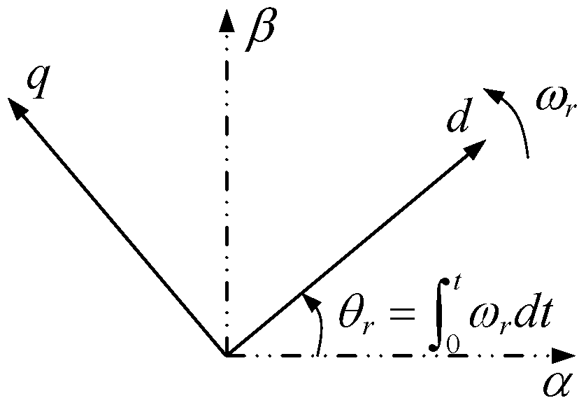
In the DTC system, the static coordinate system model is commonly used. Therefore, all the variables of BDFM must be transformed from the rotor coordinate system to the CM static coordinate system. The relationships between the rotor coordinate system ( coordinate system) and the CM static coordinate system ( coordinate system) are shown in Figure 1.
All the variables of the BDFM model Equations (1)–(3) rotate clockwise by , and the model of BDFM is obtained in the CM static coordinate system as follows:
and
The electromagnetic torque is again expressed as:
and the motion equation is the same as Equation (4).
By Equation (6), the electromagnetic torque can be re-expressed as a function of PM stator flux, CM stator flux, and rotor flux [22]:
For BDFM, the slip frequency in general is larger, so the rotor reactance is much larger than the rotor resistance, and from the third line of Equation (1), the rotor flux is small and is negligible (Because the pole pairs of PM and CM are different, the PM rotor flux and CM rotor flux are not offset in space, but in the two rotor windings, the inductive back electromotive forces are almost offset) [21]. Therefore, the electromagnetic torque of the BDFM can be simplified as:
where is the PM stator flux amplitude, is the CM stator flux amplitude, and δ is the angle difference between the PM stator flux and CM stator flux, known as the flux-angle-difference.
3. Losing Control Problem of Conventional Direct Torque Control for BDFM and Its Improved Strategy
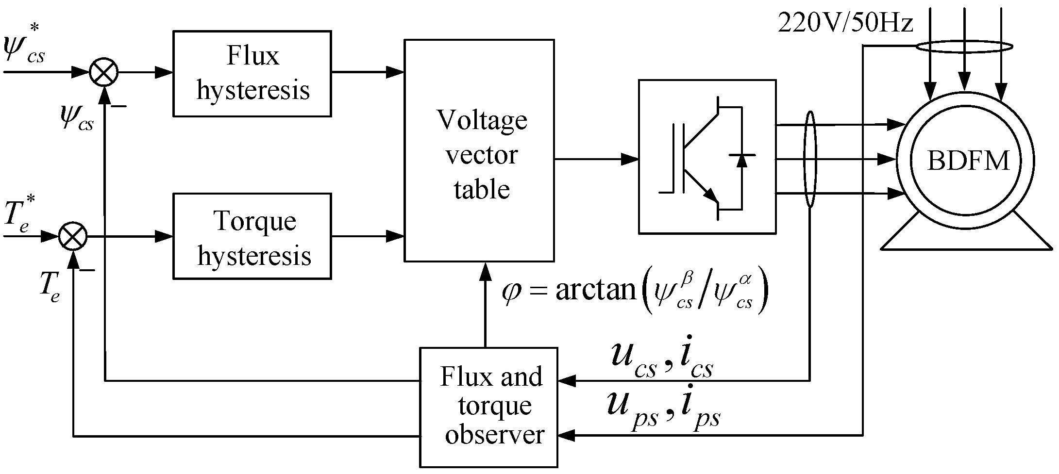
The operation principle of the BDFM’s DTC is based on the output of hysteresis comparators of the torque and CM stator flux amplitude to directly select voltage vectors of the voltage source converter, to keep the torque error and CM stator flux amplitude error within the scope of the hysteresis ring width. In the following, when the CM stator flux is in different sectors, the effects of different voltage vectors on the torque and CM stator flux amplitude are analyzed.
The torque derivative equation about time is firstly deduced as [22]:
where . Here, it is assumed that the motor is a large power motor, and the PM is powered by the mains power of 220 V/50 Hz. The voltage drop in stator resistance of PM is neglected, and the PM stator flux lags behind the stator voltage by 90° (). So, the PM stator flux amplitude is a constant, and the PM stator flux amplitude derivative , and Equation (10) becomes:
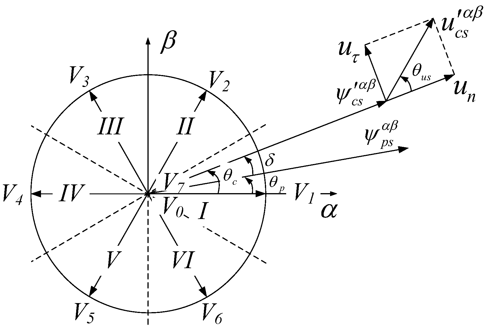
In the torque derivative expression (11), both derivatives of CM stator flux amplitude and flux-angle-difference are contained, so it is essential to express them as a function of voltage vectors. When the motor is in a steady-state operation, the two-phase static reference frame is divided into six sectors, as shown in Figure 2, where is the CM stator flux angle, is the PM stator flux angle, is the electrical angular velocity of the PM supply, and is the angle between the voltage vector and the stator flux vector of CM. For a given voltage vector , it can be decomposed into the horizontal component and vertical component of CM stator voltage in CM stator flux, and , where is the CM stator voltage vector amplitude.
Similarly to the PM, the voltage drops in stator resistance of CM are neglected. There is , so we have . Further, the derivative of CM stator flux can be expressed as:
From the above equation, we have
Obviously, the CM stator flux amplitude and speed (or phase angle) are controlled by the horizontal component and vertical component of CM stator voltage in CM stator flux, respectively. Therefore, the derivatives of CM stator flux amplitude and CM stator flux angle are obtained as:
So, the derivative equation of the flux-angle-difference is obtained as:
Here, the CM stator is supplied through a three-phase bridge converter, and the converter output voltage vectors are as follows:
where is the DC bus voltage of the converter, and corresponds to the six fundamental nonzero voltage vectors of the converter. Substituting Equation (17) into Equations (14) and (16), the derivative equations of CM stator flux amplitude and flux-angle-difference about time can be easily obtained as a function of the voltage vector as:
where is the electrical angular velocity of the CM stator. Then, substituting Equations (18) and (19) into Equation (11), the final torque derivative equation around the static working point is obtained:
where
are constant, and they are the derivative values of the flux-angle-difference and torque when the converter output voltage is the two zero voltage vectors.
The losing control problem of the BDFM’s conventional DTC (the selected voltage vectors cannot meet the control demands of flux and torque simultaneously in some time intervals, the torque ripple goes outside the hysteresis band) is analyzed specifically by Equations (18) and (20) in the following.
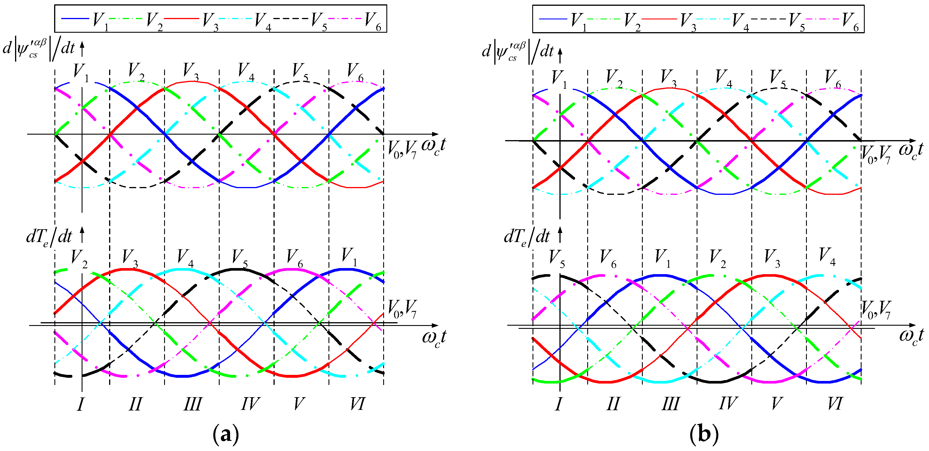
A rated power 30 kW BDFM prototype is utilized as an example whose parameters are listed in Appendix A, where the rated torque is 350 Nm, the rated flux is 0.8 Wb, and the PM stator is supplied by the constant voltage and constant frequency, 220 V/50 Hz. The derivative curves of the CM stator flux amplitude and the torque are obtained by Equations (18) and (20), as shown in Figure 3a,b. Where the CM stator flux amplitude is 0.8 Wb, the motor speed is 300 r/min (subsynchronous), and the output torques are rated torques, 350 Nm (motoring mode) and −350 Nm (generating mode). According to the derivative curves, the voltage vectors are selected. When the BDFM operates in the motoring mode, take the first sector as an example, where the voltage vectors V5, V3, V6, and V2 are selected to meet the four kinds of control requirements of the CM stator flux and the torque: decreasing in flux and torque, decreasing in flux and increasing in torque, increasing in flux and decreasing in torque, and increasing in flux and torque, respectively. Similarly, the other sectors and the generating mode voltage vector can also be selected. The voltage vector switch tables can be obtained under the motoring mode and the generating mode, as shown in Table 1 and Table 2, called the conventional DTC. The control system of conventional DTC is shown in Figure 4.
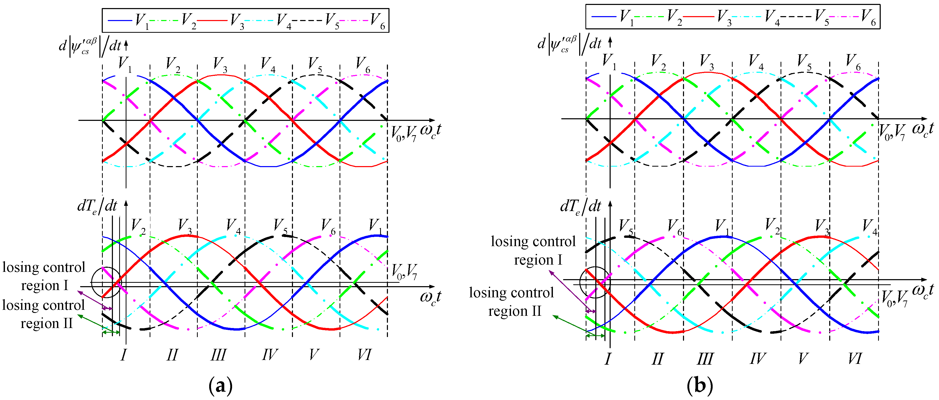
With the increase in torque, under the different operation modes, the phase angles of the flux derivative curves remain unchanged, the DC component B increases, and the torque derivative curves shift right or left relative to the flux derivative curves, as shown in Figure 5a,b. Where the CM stator flux amplitude is 0.8 Wb, the motor speed is 300 r/min (subsynchronous), and the output torque is two times the rated torque, 700 Nm (motoring mode) and −700 Nm (generating mode). The voltage vectors of the demands of four kinds of flux and torque cannot be found in the six basic voltage vectors. The choice of voltage vector can only enable the percentage of time of losing control to be as small as possible. The obtained voltage vector switch tables are same as the Table 1 and Table 2. The losing control of torque will appear at heavy load. The losing control regions are the circular regions in Figure 5a,b.
On the other hand, when the stator fluxes of BDFM remain constant, the torque can be adjusted by the flux-angle-difference. From the CM stator flux amplitude derivative Equation (18) and the flux-angle-difference derivative Equation (19), it can be seen that the DC component A is only related to the speed, but not related to the load conditions. With the increase in torque, the phase angles of the flux derivative and the flux-angle-difference derivative also remain unchanged, and they are independent of the load conditions. To solve the problem of losing control, an improved method for indirectly controlling torque is proposed by controlling the angle difference between PM stator flux and CM stator flux. In the following, the validity of the improved method will be explained by utilizing the CM stator flux amplitude and the flux-angle-difference derivative curves.
According to Equations (18) and (19), CM stator flux amplitude and flux-angle-difference derivative curves are shown in Figure 6a,b. Where CM stator flux amplitude is 0.8 Wb, the motor speed is 300 r/min (subsynchronous), and the output torques are 350 Nm (motoring mode) and −350 Nm (generating mode). Similarly, according to the derivative curves, the voltage vectors are selected to satisfy the four kinds of control requirements of the flux and the flux-angle-difference: decreasing in flux and flux-angle-difference, decreasing in flux and increasing in flux-angle-difference, increasing in flux and decreasing in flux-angle-difference, and increasing in flux and flux-angle-difference, respectively. The voltage vector switch tables can be obtained under the motoring mode and the generating mode, as shown in Table 3 and Table 4. Except for the fact that the torque hysteresis comparator is replaced with the flux-angle-difference hysteresis comparator, the selected voltage vectors are the same as in Table 1 and Table 2, called the flux-angle-difference feedback control (FADFC). The control system of the FADFC is shown in Figure 7.
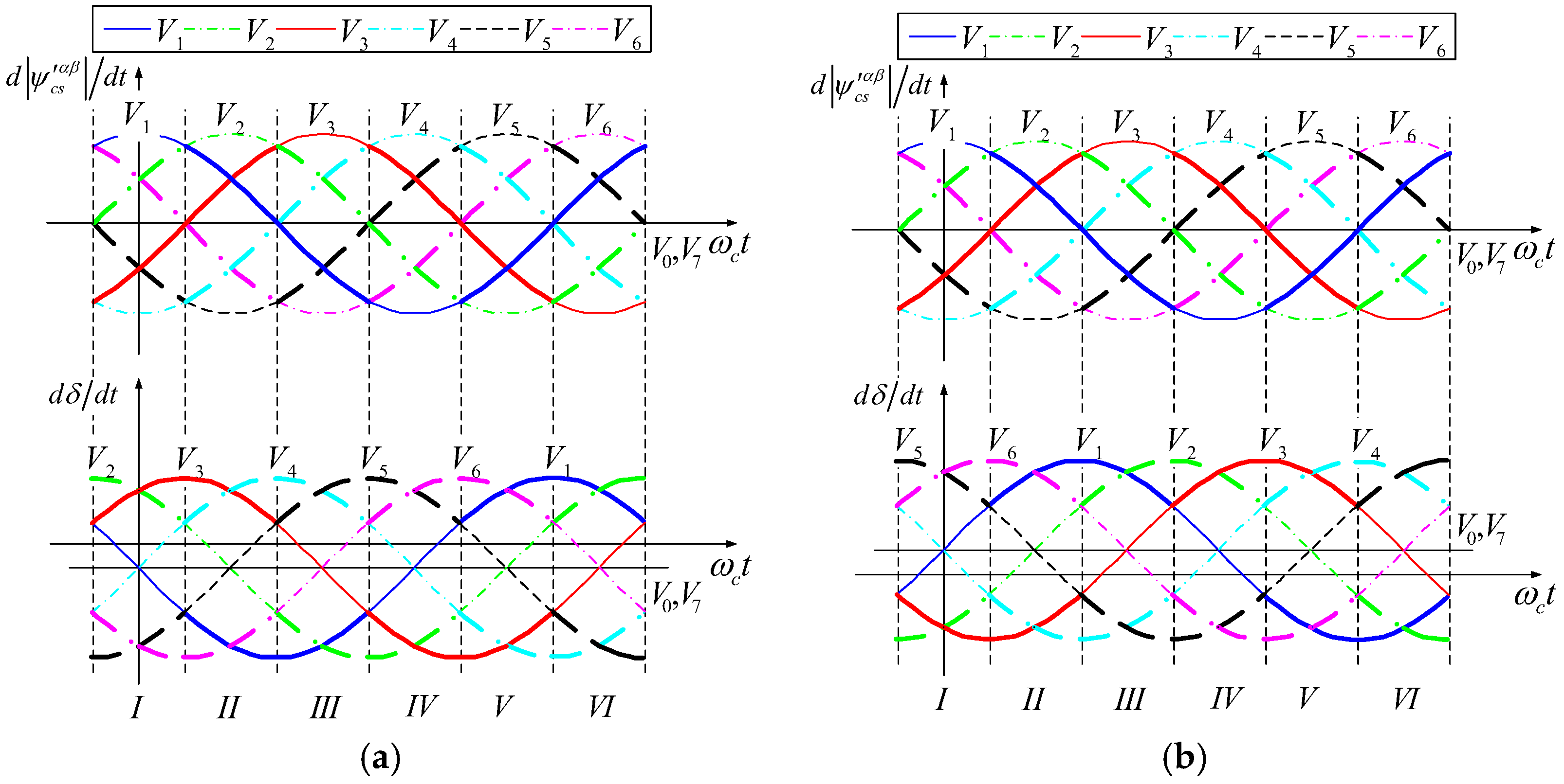
With the increase in torque, because the phase angles of the flux derivative and the flux-angle-difference derivative remain unchanged, the flux-angle-difference derivative curves will not move right or left, as shown in Figure 8a,b. With the change in speed, the DC component A will change, and the flux-angle-difference derivative curves will move down or up. From the flux-angle-difference derivative Equation (19), the amplitude of the flux-angle-difference derivative is proportional to the DC bus voltage. Therefore, before entering the field-weakening area, the selected voltage vectors can always satisfy the control requirements of the flux and the flux-angle-difference in accordance with Table 3 and Table 4.
Based on the FADFC system of Figure 7, according to the different control requirements, there are three kinds of control system design: the speed outer loop and the flux-angle-difference inner loop, the torque outer loop and the flux-angle-difference inner loop, and the three loops (the speed, the torque, and the flux-angle-difference), respectively, as shown in Figure 9.
4. Simulation Results and Analysis
In this section, the validity and dynamic performance of the proposed flux-angle-difference feedback control (FADFC) strategy have been verified by simulation experiments.
4.1. Simulation Setup
The DC bus voltage of the inverter is 500 V, the power motor stator is connected to a constant power supply, 220 V/50 Hz, and the control motor stator is supplied through a bridge inverter. From the analysis above, the conventional DTC and the proposed FADFC strategy need to know the stator fluxes by observation. This paper adopts voltage current models, and , where the pure integral is replaced with an adaptive compensation integrator, to overcome the problem of dc drifts [26]. Additionally, the torque is estimated by the vector product of currents and fluxes, presented in Equation (7). The upper and lower limits of the CM stator flux, the torque, and the flux-angle-difference hysteresis comparators are 0.05 and −0.05, 20 and −20, and 5 and −5, respectively. In order to ensure that the simulation experiments are closer to the engineering practice, the measurement time delay is considered in the simulations, the measurement of the voltage, the current, and the rotor velocity plus the filter links. The BDFM prototype specific parameters are listed in the Appendix A.
4.2. Simulation Waveforms of Direct Torque Control and Flux-Angle-Difference Feedback Control
To display the superiority of the flux-angle-difference feedback control (FADFC) more intuitively, under various kinds of operating conditions, we directly compare the control performances of the conventional DTC and the FADFC. Figure 10 and Figure 11 show the static performances of conventional DTC and FADFC, respectively.
In the simulations, only the torque loop is adopted. A dynamometer as the prime mover, which operates in the speed mode (has the speed loop), makes the BDFM work at a constant speed. The CM stator flux amplitude reference is set to 0.8 Wb, the torque reference is set to 1.5 or two times rated torque, and the motor speed is 300 r/min or 900 r/min (subsynchronous or supersynchronous).
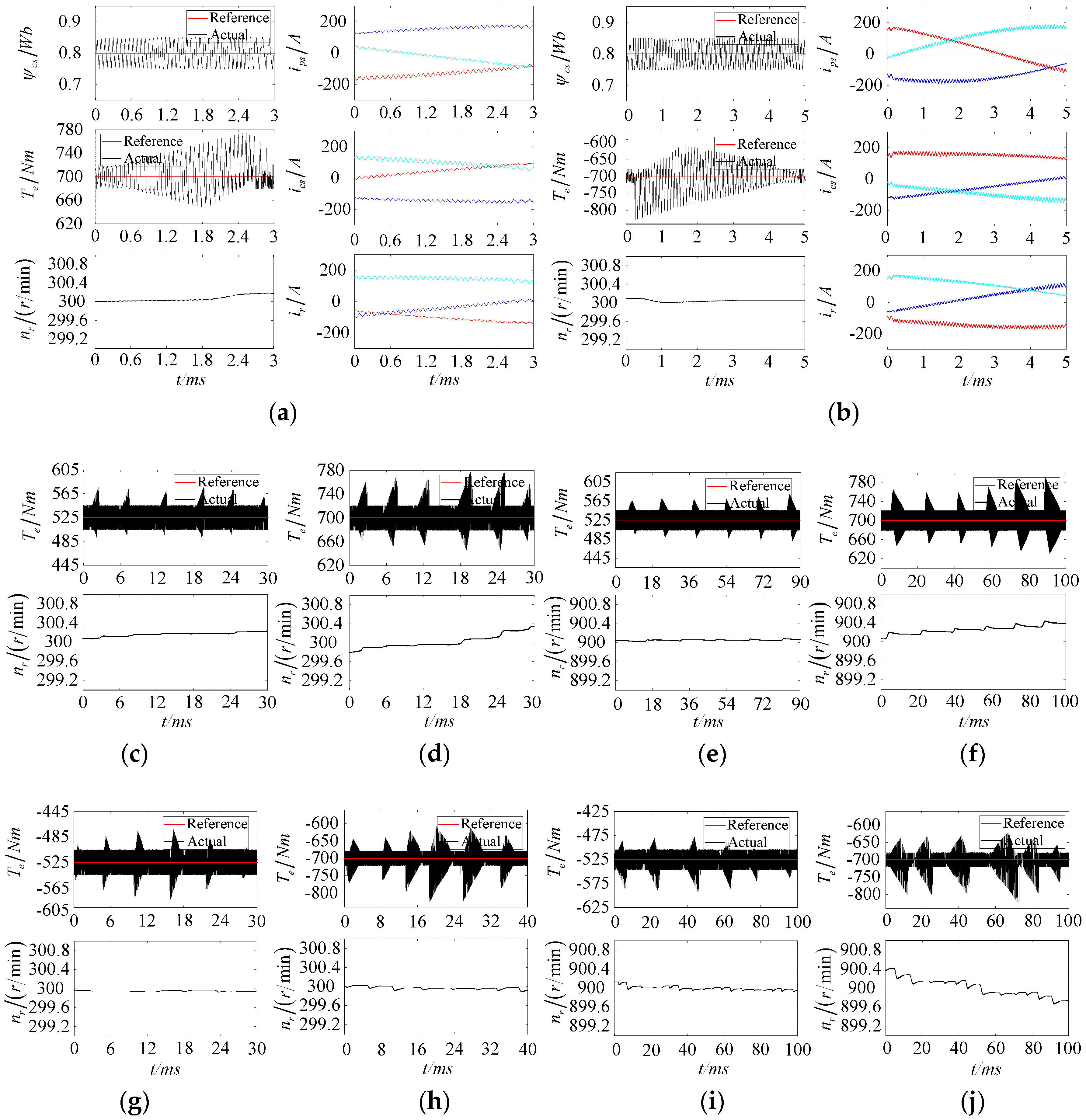
Under the different operation modes (motoring mode and generating mode), the partially enlarged simulation results of the conventional DTC are illustrated in Figure 10a,b, where all the waveforms are plotted at a steady state. It can be seen that the ripples of the CM stator flux are limited within the hysteresis band width. However, in the torque waveforms, there exist some time intervals where the torque ripples go outside the hysteresis band. During these time intervals, the torque loses control. Besides, from Figure 10c–j, under the different operation conditions, it can also be observed that in 360° electric degrees, the torque loses control in each of the six sectors, which indicates that the torque loses control in each of the six sectors. The torque losing control has two forms, during which the range of losing control gradually increases or gradually decreases, as shown in Figure 10c,d. So, whether the motor operates in motoring mode and generating mode, or subsynchronous and supersynchronous, the torque will lose control at a heavy load. With the increase of torque, the torque losing control phenomena becomes more serious, and the maximum ripple of torque is to 100 Nm. Moreover, the losing control problem continues for a longer time, and the maximum percentage of losing control time exceeds 50%.
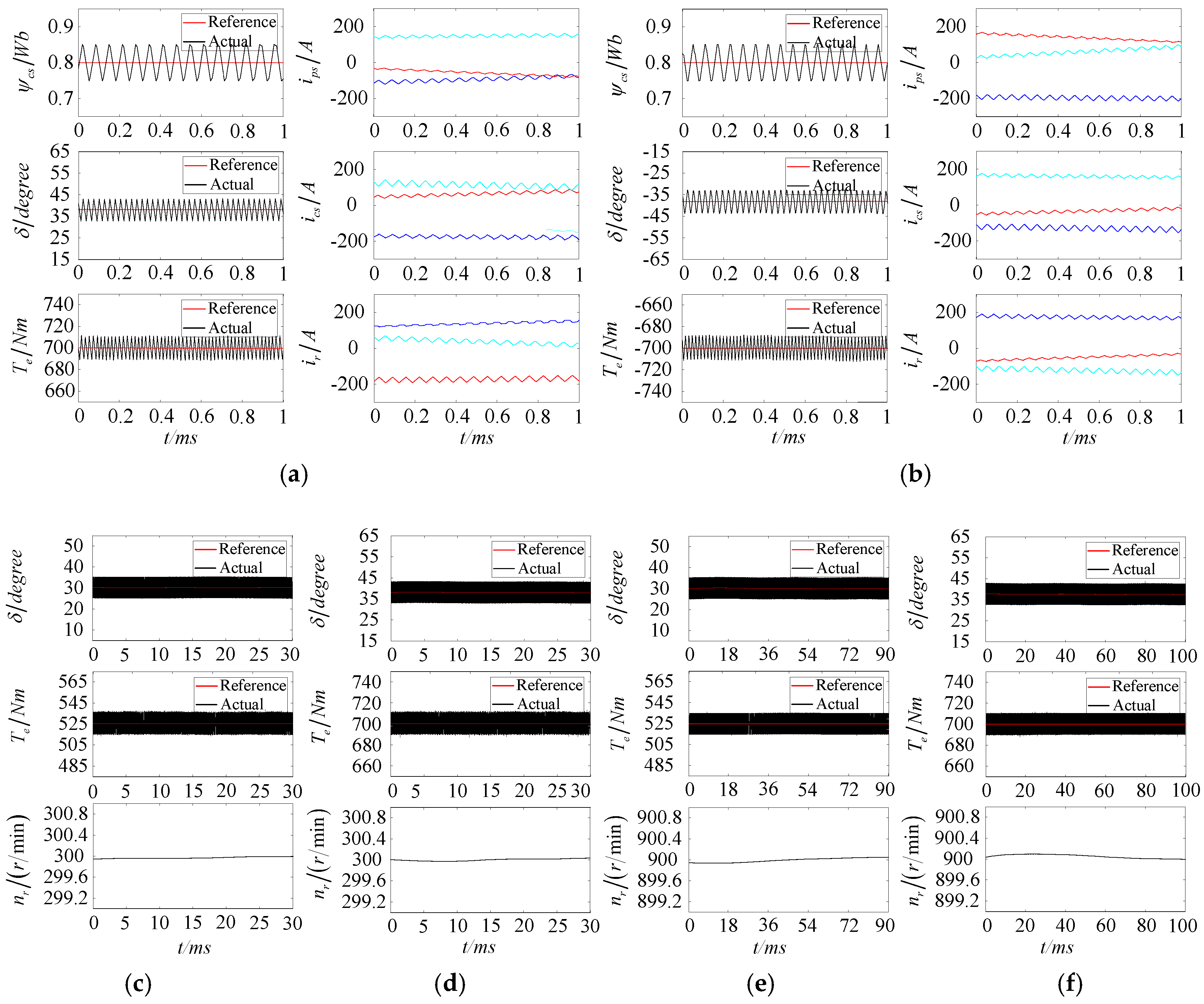
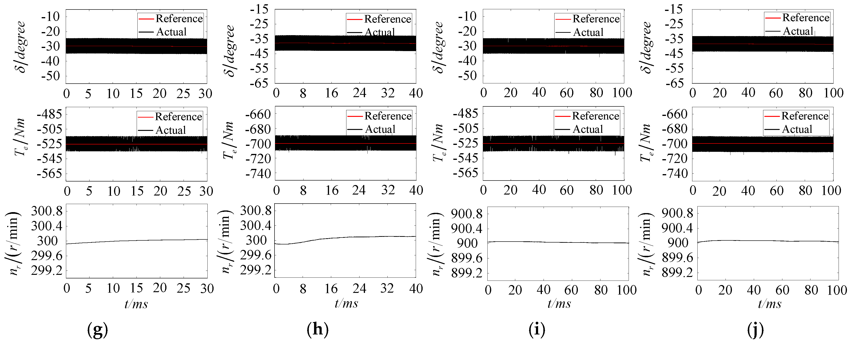
In order to make a fair comparison, the static performance of FADFC is also tested under the same operation conditions, where the motor speed is 300 r/min or 900 r/min (subsynchronous or supersynchronous). For the purpose of a convenient comparison, the CM stator flux reference and the flux hysteresis band are set to the same values as conventional DTC. The partially enlarged simulation results obtained by FADFC are shown in Figure 11a,b. It can be seen that, whether the BDFM operates in motoring mode or generating mode, the CM stator flux and the flux-angle-difference properly follow the reference value and the errors of the CM stator flux and the flux-angle-difference are strictly limited in the hysteresis band width. The torque ripples are well maintained within a proper range simultaneously. Compared with the conventional DTC, in the FADFC system, the losing control problem is not exhibited. Besides, under the different operation conditions, the motor speed, flux-angle-difference, and the torque waveforms are plotted at a steady state in several periods, as shown in Figure 11c–j. This indicates that in a wide range, the control effectiveness can be maintained by the FADFC strategy when the working conditions of the BDFM change (load torque and velocity). The proposed FADFC significantly improves the operation performance and effectively solves the losing control problem in the BDFM’s DTC system.
When CM stator flux amplitude is 0.8 Wb, from reference [27], the theoretical maximum and minimum torque curves of BDFM can be obtained, as shown in Figure 12. Under conventional DTC and FADFC, the areas of not losing control are also obtained through point-by-point simulation. It can be seen that the losing control problems of the BDFM’s conventional DTC are more serious unless the BDFM operates near the synchronous speed. Especially at zero speed, if the motor load torque amounts to less than a third of the rated load torque, the torque will lose control. Compared with the DTC, under FADFC, the area of not losing control increases significantly, and the steady state performance of the system is enhanced. The output capacity of BDFM can be increased further by the synthetic vector direct torque control (SVDTC), but the numbers of voltage vectors and the switch sector need to be increased [27].
4.3. Torque Command Responses of Flux-Angle-Difference Feedback Control
Figure 13 displays the dynamic performance of the FADFC during a sudden change in the torque command. In this simulation, the torque outer loop and the flux-angle-difference inner loop are adopted, where the CM stator flux reference is set to 0.8 Wb, the torque reference changes from 350 Nm to 800 Nm at 0.05 s, and the PI parameters of torque loop are , . During the dynamic response, it can be seen that the actual torque rapidly tracks the torque command without overshoots. In addition to this, the actual flux-angle-difference also rapidly tracks the reference value and changes from 20° to 45°. Figure 13 also shows all the waveform currents, the PM stator, the CM stator, and the rotor. Figure 13 demonstrates that the control strategy of the FADFC has a good dynamic characteristic for a sudden change of torque command. The CM stator flux amplitude tracks the reference value well, is strictly limited within the hysteresis band, and is completely unaffected by the changes of torque and motor speed.
5. Conclusions
The stator flux amplitude and speed (or phase angle) are controlled by the horizontal component and vertical component of the CM stator voltage in CM stator flux, respectively. Under the condition of constant stator flux amplitude, the torque of BDFM is proportional to the sine of the angle difference between PM stator flux and CM stator flux. Attention to these characteristics, using the flux-angle-difference hysteresis comparator instead of the torque hysteresis comparator of the conventional DTC, the design scheme of the flux-angle-difference feedback control (FADFC) is obtained. The proposed FADFC strategy can not only solve the losing control problems of the BDFM’s conventional DTC, but can also keep the advantages of DTC, such as the simple structure, less dependence on motor parameters, and strong robustness.
BDFM is a dual source supply, where the voltage current model can be used to observe the stator fluxes of PM and CM, and the drift rejection problem of pure integral has many solutions unless the BDFM operates near the synchronous speed.
The model of the BDFM is complex, and in practice its parameters are difficult to measure. Compared to the asynchronous motor, the losing control problems of the BDFM’s conventional DTC are more evident.
The models of the wound rotor BDFM and cage rotor BDFM only have a slight difference [27], so the design scheme of FADFC is also suitable for a cage rotor BDFM.
Therefore, the proposed flux-angle-difference feedback control (FADFC) scheme will have a great practical value.
Author Contributions
The idea of this paper was inspired by studying further Feng Chen’s simple think about the permanent magnet synchronous motor DTC system. Xiaoxin Hou and Chaoying Xia used flux-angle-difference to control the torque of BDFM and gave the design scheme of FADFC. All the authors wrote and revised the manuscript.
Conflicts of Interest
The authors declare no conflict of interest.
Appendix A
BDFM parameters: The rated power is 30 KW, the efficiency is 90%, the power factor is 0.8, and the rated currents 63.3 A. The shaft diameter is 105 mm. The axial length is 300 mm. The total length of the motor is 1340 mm. pp = 3, pc = 1, rps = 0.092 Ω , rcs = 0.087 Ω, lps = 0.028 H, lcs = 0.0355 H, lpm = 0.027 H, lcm = 0.0347 H, rr = 0.04 Ω, and ll = 0.0635 H.
References
- Abdi, E.; McMahon, R.; Malliband, P. Performance analysis and testing of a 250 kW medium-speed brushless doubly-fed induction generator. IET Renew. Power Gener. 2013, 6, 631–638. [Google Scholar] [CrossRef]
- Tohidi, S.; Tavner, P.; McMahon, R. Low voltage ride-through of DFIG and brushless DFIG: Similarities and differences. Electr. Power Syst. Res. 2014, 110, 64–72. [Google Scholar] [CrossRef]
- Tohidi, S.; Oraee, H.; Zolghadri, M.R. Analysis and enhancement of low-voltage ride-through capability of brushless doubly fed induction generator. IEEE Trans. Ind. Electron. 2013, 3, 1146–1155. [Google Scholar] [CrossRef] [Green Version]
- Shao, S.; Long, T.; Abdi, E. Dynamic control of the brushless doubly fed induction generator under unbalanced operation. IEEE Trans. Ind. Electron. 2013, 6, 2465–2476. [Google Scholar] [CrossRef]
- Gorginpour, H.; Oraee, H.; McMahon, R.A. Electromagnetic-thermal design optimization of the brushless doubly fed induction generator. IEEE Trans. Ind. Electron. 2014, 4, 1710–1721. [Google Scholar] [CrossRef]
- Liu, Y.; Ai, W.; Chen, B.; Chen, K.; Luo, G. Control design and experimental verification of the brushless doubly-fed machine for stand-alone power generation applications. IET Electr. Power Appl. 2016, 1, 25–35. [Google Scholar] [CrossRef]
- Zhou, D.S.; Spee, R. Synchronous frame model and decoupled control development for doubly-fed machines. In Proceedings of the 25th Annual IEEE Power Electronics Specialists Conference, Taipei, China, 20–25 June 1994. [Google Scholar]
- Zhou, D.; Spee, R.; Alexander, G.C.; Wallace, A.K. A simplified method for dynamic control of brushless double-fed machines. In Proceedings of the 1996 IEEE IECON 22nd International Conference on Industrial Electronics, Control, and Instrumentation, Taipei, China, 5–10 August 1996; pp. 946–951. [Google Scholar]
- Poza, J.; Oyarbide, E.; Roye, D.; Rodriguez, M. Unified reference frame dq model of the brushless doubly fed machine. IEE Proc. Electr. Power Appl. 2006, 153, 726–734. [Google Scholar] [CrossRef]
- Poza, J.; Oyarbide, E.; Sarasola, I. Vector control design and experimental evaluation for the brushless doubly fed machine. IET Electr. Power Appl. 2009, 4, 247–256. [Google Scholar] [CrossRef]
- Shao, S.Y.; Abdi, E.; Barati, F.; McMahon, R. Stator-flux-oriented vector control for brushless doubly fed induction generator. IEEE Trans. Ind. Electron. 2009, 10, 4220–4228. [Google Scholar] [CrossRef]
- Barati, F.; McMahon, R.; Shao, S. Generalized vector control for brushless doubly fed machines with nested-loop rotor. IEEE Trans. Ind. Electron. 2013, 6, 2477–2485. [Google Scholar] [CrossRef]
- Xia, C.Y.; Guo, H.Y. Feedback linearization control approach for brushless double-fed machine. Int. J. Precis. Eng. Manuf. 2015, 8, 1699–1709. [Google Scholar] [CrossRef]
- Abad, G.; Rodríguez, M.Á.; Poza, J. Two-level VSC based predictive direct torque control of the doubly fed induction machine with reduced torque and flux ripples at low constant switching frequency. IEEE Trans. Power Electron. 2008, 3, 1050–1061. [Google Scholar] [CrossRef]
- Brando, G.; Dannier, A.; Pizzo, A. Generalised look-up table concept for direct torque control in induction drives with multilevel inverters. IET Electr. Power Appl. 2015, 8, 556–567. [Google Scholar] [CrossRef]
- Jovanovic, M. Sensored and sensorless speed control methods for brushless doubly fed reluctance motors. IET Electr. Power Appl. 2009, 6, 503–513. [Google Scholar] [CrossRef]
- Petronijević, M.; Mitrović, N.; Kostić, V.; Banković, B. An Improved Scheme for Voltage Sag Override in Direct Torque Controlled Induction Motor Drives. Energies 2017, 5, 663. [Google Scholar] [CrossRef]
- Alsofyani, I.; Idris, N. Simple flux regulation for improving state estimation at very low and zero speed of a speed sensorless direct torque control of an induction motor. IEEE Trans. Power Electron. 2016, 4, 3027–3035. [Google Scholar] [CrossRef]
- Sebtahmadi, S.; Pirasteh, H.; Kaboli, A. A 12-sector space vector switching scheme for performance improvement of matrix-converter-based DTC of IM drive. IEEE Trans. Power Electron. 2015, 7, 3804–3817. [Google Scholar] [CrossRef]
- Sutikno, T.; Idris, N.; Jidin, A. An improved FPGA implementation of direct torque control for induction machines. IEEE Trans. Ind. Inform. 2013, 3, 1280–1290. [Google Scholar] [CrossRef]
- Yousefi, B.; Soleymani, S.; Mozafari, B.; Gholamian, S.A. Speed Control of Matrix Converter-Fed Five-Phase Permanent Magnet Synchronous Motors under Unbalanced Voltages. Energies 2017, 10, 1509. [Google Scholar] [CrossRef]
- Sarasola, I.; Poza, J.; Rodríguez, M.Á.; Abad, G. Direct torque control design and experimental evaluation for the brushless doubly fed machine. Energy Convers. Manag. 2011, 2, 1226–1234. [Google Scholar] [CrossRef]
- Sarasola, I.; Poza, J.; Rodríguez, M.Á. Predictive direct torque control for brushless doubly fed machine with reduced torque ripple at constant switching frequency. In Proceedings of the 2007 IEEE International Symposium on Industrial Electronics, Vigo, Spain, 4–7 June 2007. [Google Scholar]
- Fattahi, S.J.; Khayyat, A.A. Direct torque control of brushless doubly-fed induction machines using fuzzy logic. In Proceedings of the 2011 IEEE Ninth International Conference on Power Electronics and Drive Systems (PEDS), Singapore, 5–8 December 2011. [Google Scholar]
- Zhang, A.L.; Wang, X.; Jia, W.X.; Ma, Y. Indirect stator-quantities control for the brushless doubly fed induction machine. IEEE Trans. Power Electron. 2014, 3, 1392–1401. [Google Scholar] [CrossRef]
- Hu, J.; Wu, B. New integration algorithms for estimating motor flux over a wide speed range. IEEE Trans. Power Electron. 1998, 5, 967–977. [Google Scholar]
- Xia, C.; Hou, X. Study on the Static Load Capacity and Synthetic Vector Direct Torque Control of Brushless Doubly Fed Machines. Energies 2016, 11, 966. [Google Scholar] [CrossRef]
Figure 1.
Relationships between the rotor coordinate system and CM static coordinate system.

Figure 2.
Space vector diagram of conventional DTC.

Figure 3.
CM stator flux amplitude and torque derivative curves (rated torque) (a) Motoring mode (Te = 350 Nm); (b) Generating mode (Te = −350 Nm).
Figure 3.
CM stator flux amplitude and torque derivative curves (rated torque) (a) Motoring mode (Te = 350 Nm); (b) Generating mode (Te = −350 Nm).

Figure 4.
Control system of conventional DTC.

Figure 5.
CM stator flux amplitude and torque derivative curves (two times rated torque) (a) Motoring mode (Te = 700 Nm); (b) Generating mode (Te = −700 Nm).
Figure 5.
CM stator flux amplitude and torque derivative curves (two times rated torque) (a) Motoring mode (Te = 700 Nm); (b) Generating mode (Te = −700 Nm).

Figure 6.
CM stator flux amplitude and flux-angle-difference derivative curves (rated torque) (a) Motoring mode (Te = 350 Nm, δ = 20°); (b) Generating mode (Te = −350 Nm, δ = −20°).
Figure 6.
CM stator flux amplitude and flux-angle-difference derivative curves (rated torque) (a) Motoring mode (Te = 350 Nm, δ = 20°); (b) Generating mode (Te = −350 Nm, δ = −20°).

Figure 7.
Control system of FADFC.
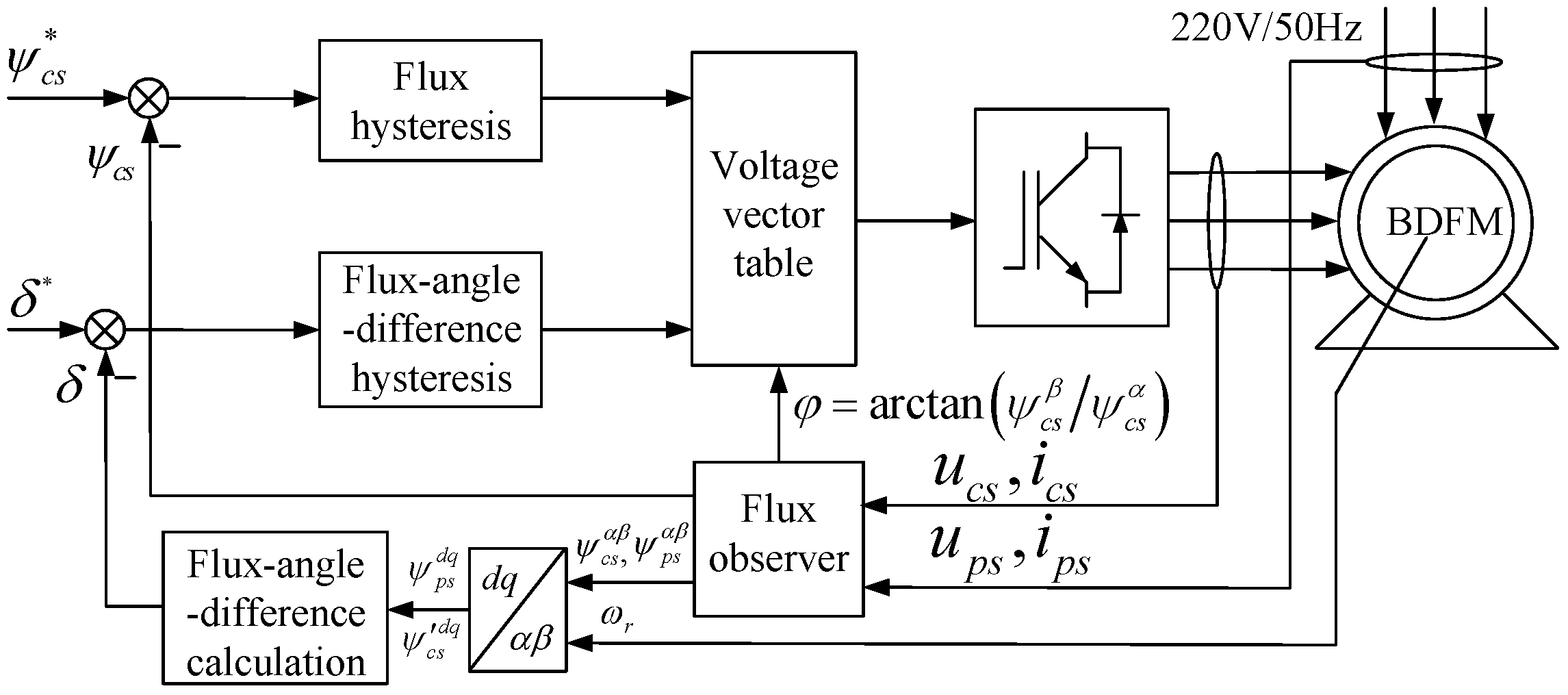
Figure 8.
CM stator flux amplitude and flux-angle-difference derivative curves (2 times rated torque) (a) Motoring mode (Te = 700 Nm, δ = 38°); (b) Generating mode (Te = −700 Nm, δ = −38°).
Figure 8.
CM stator flux amplitude and flux-angle-difference derivative curves (2 times rated torque) (a) Motoring mode (Te = 700 Nm, δ = 38°); (b) Generating mode (Te = −700 Nm, δ = −38°).
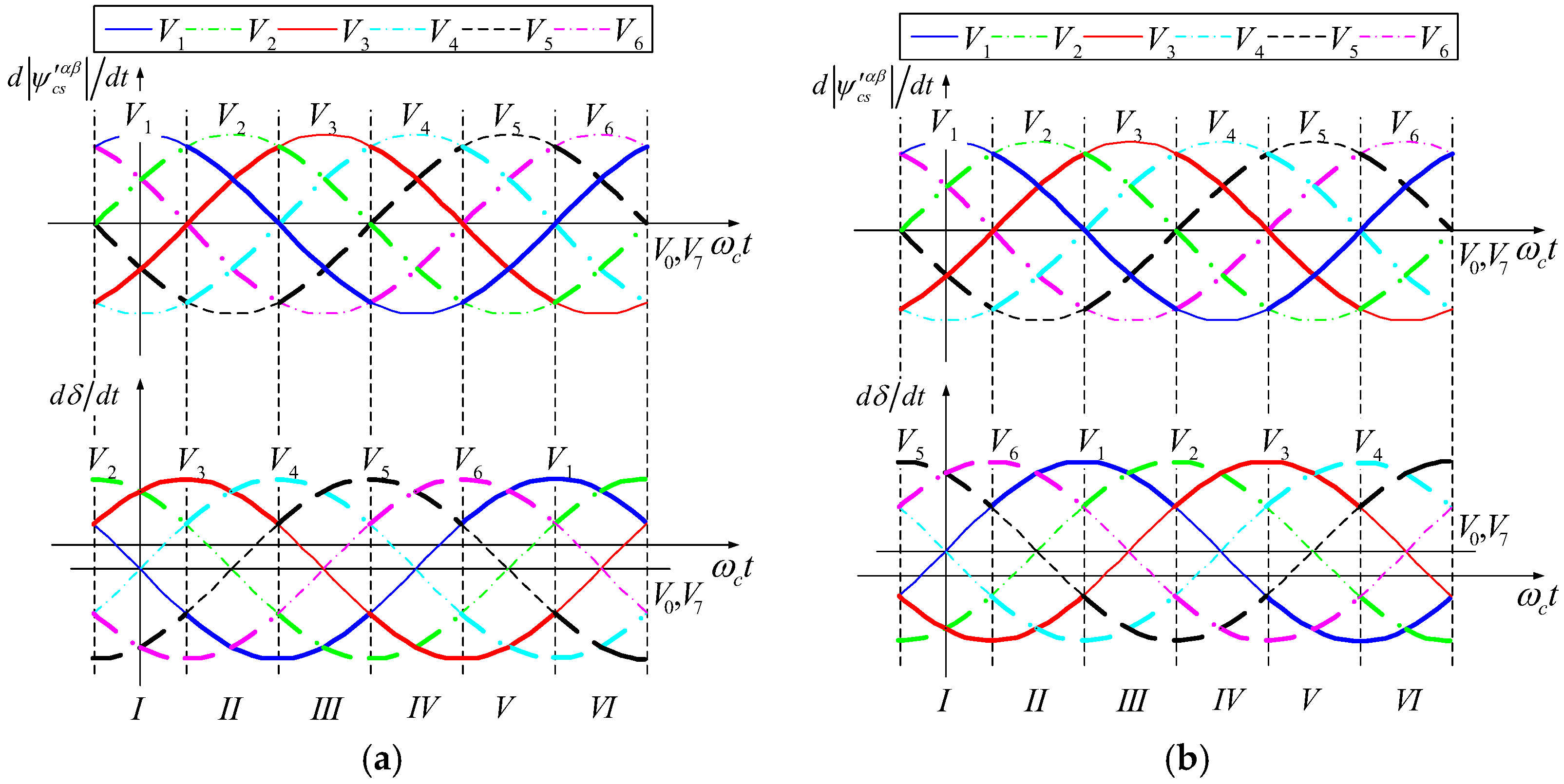
Figure 9.
Three kinds of control system design based on FADFC (a) Speed outer loop and flux-angle-difference inner loop (b) Torque outer loop and flux-angle-difference inner loop (c) Three loops.
Figure 9.
Three kinds of control system design based on FADFC (a) Speed outer loop and flux-angle-difference inner loop (b) Torque outer loop and flux-angle-difference inner loop (c) Three loops.
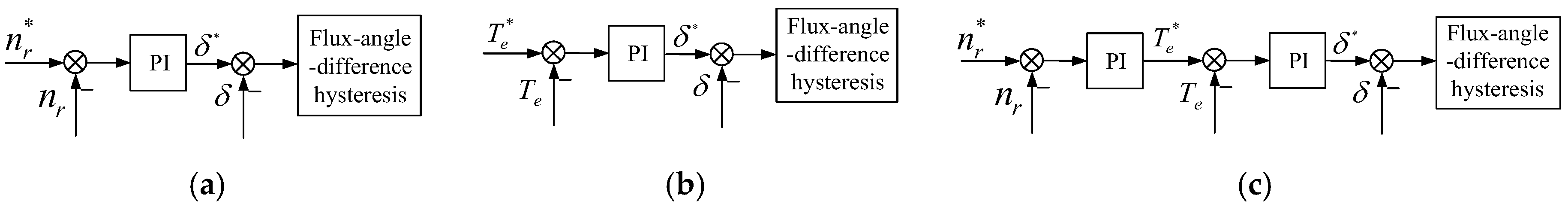
Figure 10.
Simulation waveforms of conventional DTC (1.5 and two times rated torque) Partially enlarged: (a) Te = 700 Nm, nr = 300 r/min (b) Te = −700 Nm, nr = 300 r/min; Periodogram: (c) Te = 525 Nm, nr = 300 r/min (d) Te = 700 Nm, nr = 300 r/min (e) Te = 525 Nm, nr = 900 r/min (f) Te = 700 Nm, nr = 900 r/min (g) Te = −525 Nm, nr = 300 r/min (h) Te = −700 Nm, nr = 300 r/min (i) Te = −525 Nm, nr = 900 r/min (j) Te = −700 Nm, nr = 900 r/min.

Figure 11.
Simulation waveforms of FADFC (1.5 and two times rated torque) Partially enlarged: (a) Te = 700 Nm, nr = 300 r/min (b) Te = −700 Nm, nr = 300 r/min; Periodogram: (c) Te = 525 Nm, nr = 300 r/min (d) Te = 700, Nm, nr = 300 r/min (e) Te = 525 Nm, nr = 900 r/min (f) Te = 700 Nm, nr = 900 r/min (g) Te = −525 Nm, nr = 300 r/min (h) Te = −700 Nm, nr = 300 r/min (i) Te = −525 Nm, nr = 900 r/min (j) Te = −700 Nm, nr = 900 r/min.


Figure 12.
Losing control ranges under conventional DTC.
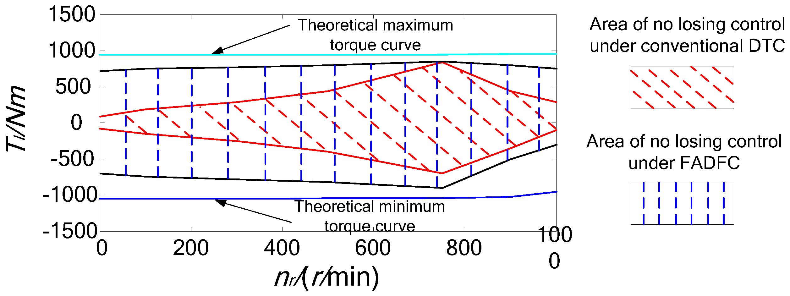
Figure 13.
Dynamic performance of FADFC.


Table 1.
Voltage vector switch table (conventional DTC motoring mode).
| Output of Hysteresis Comparator | Six Sectors | ||||||
|---|---|---|---|---|---|---|---|
| Flux | Torque | I | II | III | IV | V | VI |
| −1 | −1 | V5 | V6 | V1 | V2 | V3 | V4 |
| 1 | V3 | V4 | V5 | V6 | V1 | V2 | |
| 1 | −1 | V6 | V1 | V2 | V3 | V4 | V5 |
| 1 | V2 | V3 | V4 | V5 | V6 | V1 | |
Table 2.
Voltage vector switch table (conventional DTC generating mode).
| Output of Hysteresis Comparator | Six Sectors | ||||||
|---|---|---|---|---|---|---|---|
| Flux | Torque | I | II | III | IV | V | VI |
| −1 | −1 | V3 | V4 | V5 | V6 | V1 | V2 |
| 1 | V5 | V6 | V1 | V2 | V3 | V4 | |
| 1 | −1 | V2 | V3 | V4 | V5 | V6 | V1 |
| 1 | V6 | V1 | V2 | V3 | V4 | V5 | |
Where, “1” and “−1” indicate the increased and decreased flux or torque, respectively.
Table 3.
Voltage vector switch table (FADFC motoring mode).
| Output of Hysteresis Comparator | Six Sectors | ||||||
|---|---|---|---|---|---|---|---|
| Flux | Flux-Angle-Difference | I | II | III | IV | V | VI |
| −1 | −1 | V5 | V6 | V1 | V2 | V3 | V4 |
| 1 | V3 | V4 | V5 | V6 | V1 | V2 | |
| 1 | −1 | V6 | V1 | V2 | V3 | V4 | V5 |
| 1 | V2 | V3 | V4 | V5 | V6 | V1 | |
Table 4.
Voltage vector switch table (FADFC generating mode).
| Output of Hysteresis Comparator | Six Sectors | ||||||
|---|---|---|---|---|---|---|---|
| Flux | Flux-Angle-Difference | I | II | III | IV | V | VI |
| −1 | −1 | V3 | V4 | V5 | V6 | V4 | V2 |
| 1 | V5 | V6 | V1 | V2 | V3 | V4 | |
| 1 | −1 | V2 | V3 | V4 | V5 | V6 | V1 |
| 1 | V6 | V1 | V2 | V3 | V4 | V5 | |
Where, “1” and “−1” indicate the increased and decreased flux or flux-angle-difference, respectively.
© 2018 by the authors. Licensee MDPI, Basel, Switzerland. This article is an open access article distributed under the terms and conditions of the Creative Commons Attribution (CC BY) license (http://creativecommons.org/licenses/by/4.0/).
Share and Cite
MDPI and ACS Style
Xia, C.; Hou, X.; Chen, F. Flux-Angle-Difference Feedback Control for the Brushless Doubly Fed Machine. Energies 2018, 11, 71. https://doi.org/10.3390/en11010071
AMA Style
Xia C, Hou X, Chen F. Flux-Angle-Difference Feedback Control for the Brushless Doubly Fed Machine. Energies. 2018; 11(1):71. https://doi.org/10.3390/en11010071
Chicago/Turabian StyleXia, Chaoying, Xiaoxin Hou, and Feng Chen. 2018. "Flux-Angle-Difference Feedback Control for the Brushless Doubly Fed Machine" Energies 11, no. 1: 71. https://doi.org/10.3390/en11010071
Note that from the first issue of 2016, this journal uses article numbers instead of page numbers. See further details here.