1. Introduction
Many power systems around the world are characterized by weak longitudinal structures. These power systems, also known as longitudinal power systems (LPS), usually have a radial configuration (with multiple infeed), with generation areas electrically distant from concentrated load centers, connected through long transmission lines, which leads to weak connections between those areas [
1,
2,
3]. Examples of LPS are found in Chile, Mexico, Peru, Taiwan, Finland, Israel, Australia, England, and Italy, among others.
Due to their longitudinal structure and characteristics, LPS are prone to face different stability problems in cases in which meshed (robust) networks would not. This is because even small changes in active and reactive power flows/injections might lead to significant changes in phase angles and voltage magnitudes [
1]. Transmission system operators (TSOs) of this kind of systems are familiarized with these critical situations. Indeed, they know those cases in which traditional remedial actions will not be able to save the system from a total blackout. In those circumstances, splitting the system in different islands is the only remedial action to avoid the total collapse of the system. Moreover, given the sparse configuration, in LPS it is relatively common to operate in electrical islands under severe disturbances [
1].
Given the special operational challenges of LPS, corrective and preventive actions taken by TSOs to guarantee the system stability can be of significant importance. In this context, synchronized measurements arise as a real alternative to provide real-time data from the system, such as wide-area measurements systems (WAMS) [
4]. In contrast to the well-known supervisory control and data acquisition (SCADA) systems, WAMS provide consistently time-synchronized and time-aligned phasor measurements with higher reporting rates [
4,
5]. Monitoring key variables such as phase angles using WAMS, may provide better ways to detect and control transient instabilities [
4,
5,
6] and thus prevent possible blackouts. In this context, out-of-step (OOS) protection functions are commonly used to maintain the system integrity [
7]. These functions detect out-of-step conditions and take remedial actions such as separating the affected areas from the rest of the system, while minimizing load shedding and maintaining the continuity of the service [
8,
9].
Given the advantages of WAMS and the usefulness of OOS protection functions in LPS, this work proposes an active splitting control scheme based on a wide-area monitoring, protection and control (WAMPC) system using local and remote synchrophasor measurements. The proposed control scheme uses a modified OOS algorithm with the angle difference method to detect possible instable system trajectories, and then split it accordingly. To accomplish this, the knowledge of the TSOs is exploited not only to identify particular contingencies that may led to a total collapse, but also to identify the places where a system must be separated in case of those critical contingencies. The control scheme was tested on a detailed dynamic model of the Central Interconnected System (CIS) of Chile, a good example of extreme LPS [
10].
This paper is organized as follows:
Section 2 specifies the main characteristics of LPS.
Section 3 summarizes two synchrophasor based approaches of the out-of-step detection method.
Section 4 presents the proposed scheme including the proposed methodology for tuning its parameters.
Section 5 and
Section 6 present the case study and the obtained results, respectively. Finally,
Section 7 draws the main conclusions of this research.
2. Electrical Characteristics of LPS
Short circuit capacity (SCC) is a nodal indicator of robustness of any power system: the higher the value of the SCC, the higher the network robustness at the pertinent node. The SCC is computed as the inverse of the positive sequence equivalent impedance seen from the node under study. In comparison to robust networks, the SCC levels in LPS are usually low [
1,
2], indicating the weak nature of these system configurations.
Table 1 summarizes typical values for SCC levels in Europe and Chile: an example of extreme LPS.
LPS are also very sensitive to active and reactive power changes [
1]. To see this, let consider the fast decoupled load flow equations in a network with
N nodes [
12]:
where the vectors
and
(with dimension of
) represent the changes in phase angles and voltage magnitudes, respectively, at each bus of the system; and
and
(also with dimension of
), respectively, contain the active and reactive power injections at each node. Equations (
1) and (
2) give a relationship between phase angles and active power injections and between voltage magnitudes and reactive power injections. In the case of LPS, the values of the coefficient included in the entries of the matrices
and
are usually large, meaning that even small changes in active and reactive power injections can lead to significant changes in phase angles and voltage magnitudes [
1]. By contrast, in robust (meshed) networks, these values are small and hence only small changes are expected.
Due to their longitudinal structure and characteristics, LPS are prone to face different stability problems. Among the most critical stability concerns are those related to transient and voltage stability [
3], including low frequency oscillations (from a small signal stability viewpoint), and voltage collapse. Indeed, sustained low frequency oscillations [
13,
14,
15,
16] as well as voltage instability situations [
17,
18,
19] have been reported in several power systems with longitudinal structure.
3. Out-of-Step Detection Methods Based on Synchrophasors
When a loss of synchronism occurs, either between a group of generators and the rest of the system, or between interconnected power systems, a number of generators start to run at slightly different speeds [
20]. This phenomenon is directly reflected in changes in the phase angles of the positive-sequence voltage (PSV) of the network [
21,
22]. In this context, since existing WAMPC technologies allows the monitoring of these variables in real time, different OOS approaches have been proposed in the literature using synchrophasor measurements. One method consists in comparing the absolute angle difference of the PSV between two phasor measurement units (PMUs) located at different buses, against a predefined threshold [
23]. Let
denote the angular difference between the two busbars being analyzed. If the absolute value of
is greater than a threshold, it is assumed that the system is following an instable trajectory. Otherwise, the system is stable. Different approaches of this algorithm have been presented in [
9,
23,
24,
25], all of them using Equations (
3) and (
4).
where
and
are the phase angles of the PSV measured by PMU1 and PMU2, respectively, at the
k processing interval; and
is the maximum threshold for the angular difference between two busbars.
Another method based on synchrophasor measurements is the predictive out-of-step tripping (OOST) scheme proposed in [
9,
23,
24,
25]. Let
and
respectively denote the slip frequency and the acceleration. Both
and
are computed from the value of the angle difference
. In this method, a stability region in the
plane is identified. Consequently, if a trajectory of the power system (e.g., a power swing) tends towards the boundaries of the stable region, or reaches the area outside the (stable) region, an OOS condition is assumed and corrective actions are taken accordingly. Mathematically,
and
are calculated as follows:
where
is the angle difference obtained using Equation (
3) at the
k processing interval; and MRATE is the synchrophasor message rate. From Equations (
5) and (
6), it can be seen that
and
are the first and second derivative of the angle difference
, respectively.
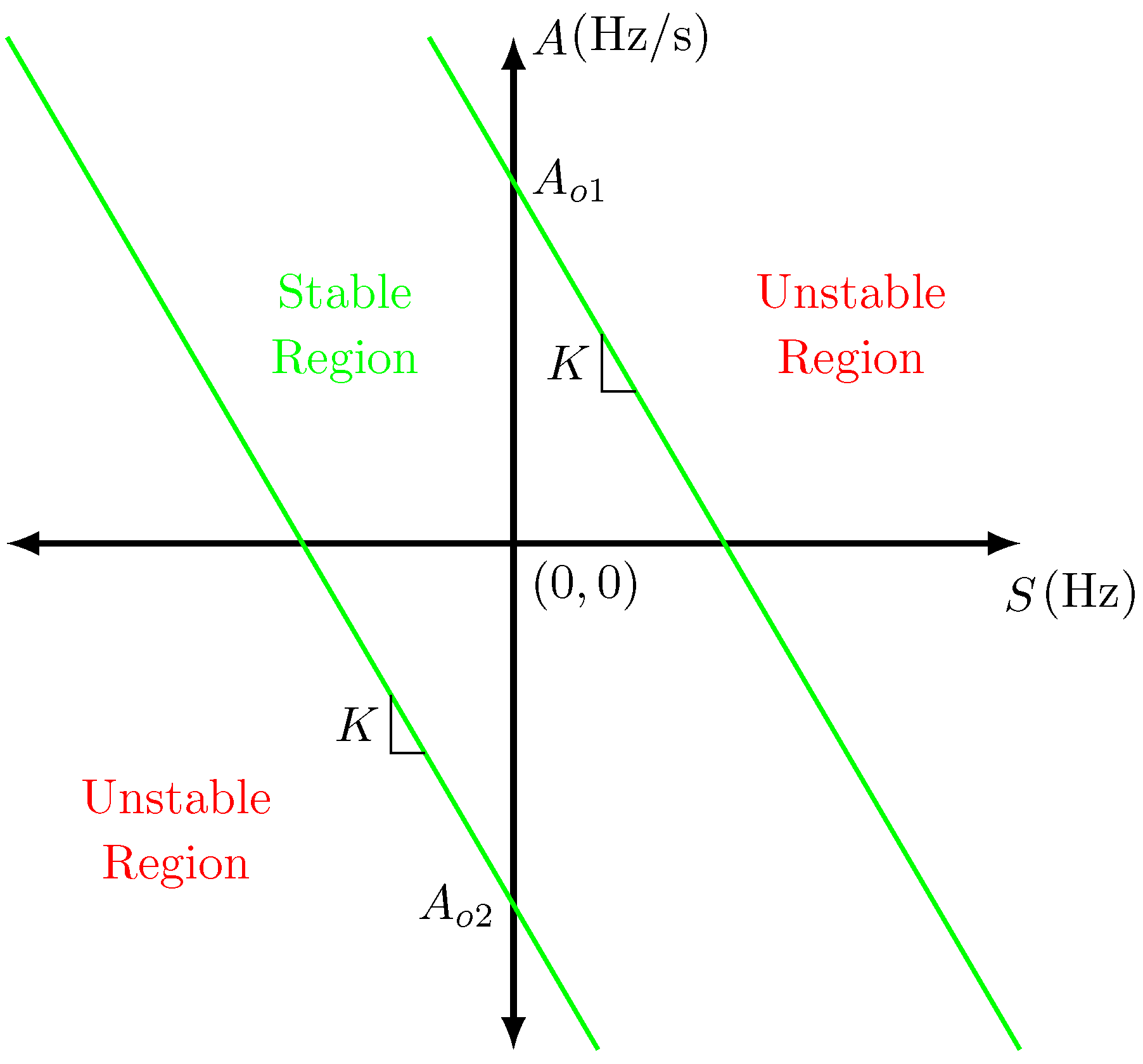
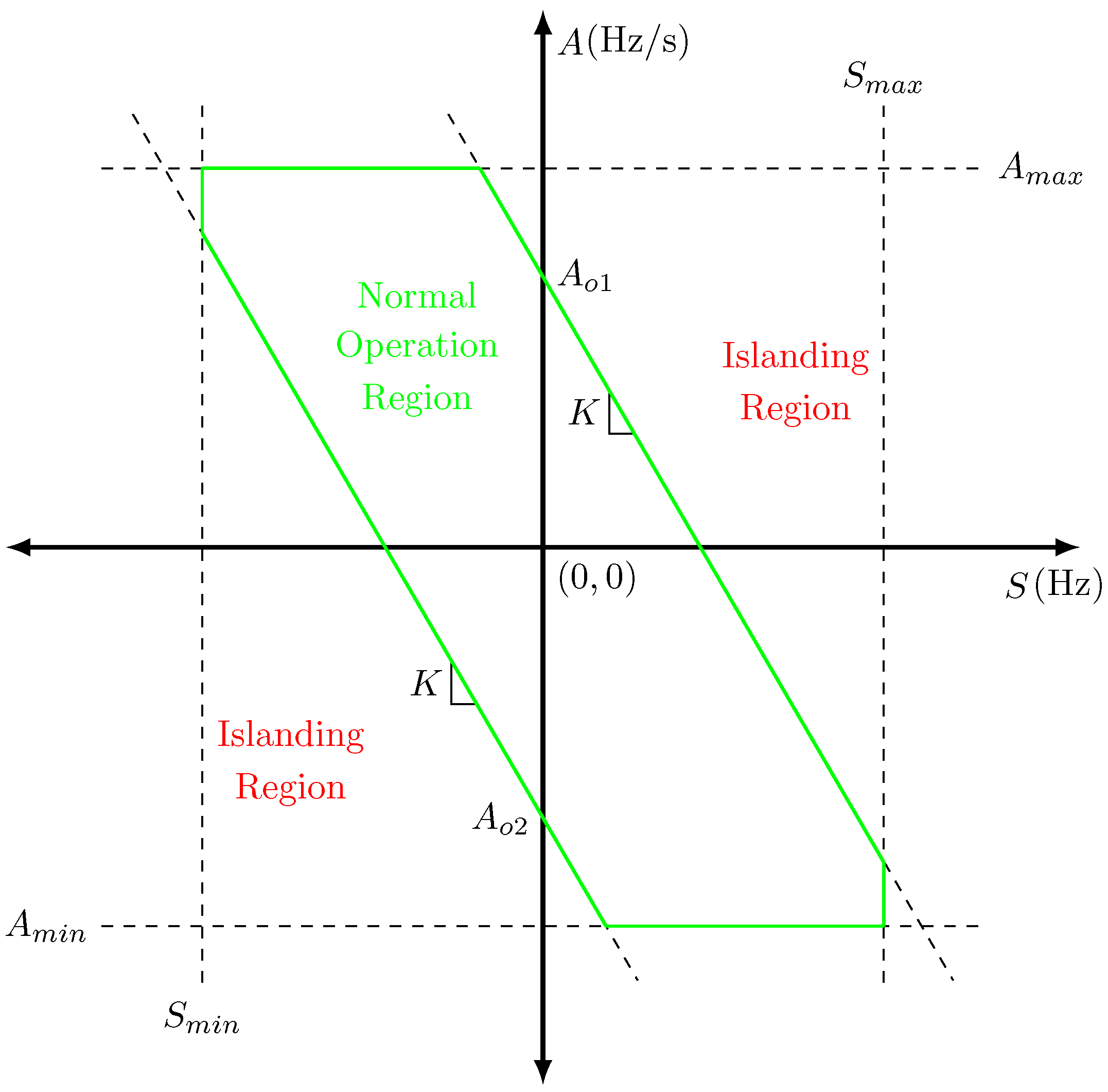
Figure 1 shows the characteristic of an OOST scheme in the
plane.
The unstable region of the OOST characteristic is defined by Equations (
7) and (
8).
where
K is a slope constant of the power system and the constants
and
are the acceleration offset values. The values of
K,
and
have to be determined based on the characteristics of the system and/or using dynamic simulations under different operating points and contingencies [
23].
4. Proposal for Active Splitting in LPS
When an OOS condition is detected, different remedial actions, such as tripping the faulted generation units [
6] or shedding load [
22], may be taken in order to maintain the system stability or at least to limit the cascading effects in the network [
8,
9]. Nevertheless, these remedial actions could fail to lead the system to a secure state [
26]. In these critical cases, a last remedial action to save—at least—some pre-identified areas is to split the network at specific locations in order to create system islands. The islands must have a balance between generation and load demand and should remain in synchronism [
8,
22]. In this context, controlled power system separation (also known as active splitting) is a protection scheme that prevents large scale power system blackouts under severe contingencies [
27]. The main idea is to intentionally split transmission networks into islands of load with matched generation at proper splitting points by opening previously selected transmission lines [
28]. The areas must be separated from each other quickly [
8] and this must be precise and reliable, since it normally leads to significant structural changes in the network [
9].
Given the sparse configuration of LPS, it is relatively common to operate in electrical islands under severe disturbances [
1]. The cases of Australia [
29] and Chile [
30] are good examples of such type of operation, and support the fact that TSOs have the knowledge and experience of what areas may operate as island maintaining the stability after the splitting. Nevertheless, in cases where the separated systems have a generation–load imbalance, it may be necessary to shed selected loads and/or trip generators [
31] in order to sustain frequency stability.
4.1. Active Splitting Control Scheme
In this work, the OOST algorithm explained in
Section 3 was modified and accordingly combined with the angle difference scheme to propose an improved active splitting scheme (ASS) especially suitable for LPS. Since phase angles in a LPS may change drastically even when small changes in active power occur (see
Section 2 for details), it seems appropriate to further limit the normal operation region shown in
Figure 1. To do this, upper and lower boundaries for the slip frequency and acceleration in the
plane are included, as shown in
Figure 2. These boundaries use Equations (
9) and (
10) to detect an unstable operating point.
Due to high values reached by the slip frequency and acceleration during unstable swings or OOS conditions in LPS, these boundaries may detect the instability before the trajectory
crosses the traditional OOST limits. Thus, with the modified OOST shown in
Figure 2 (named MOOST), it is feasible to take faster remedial actions than with a traditional OOST [
32].
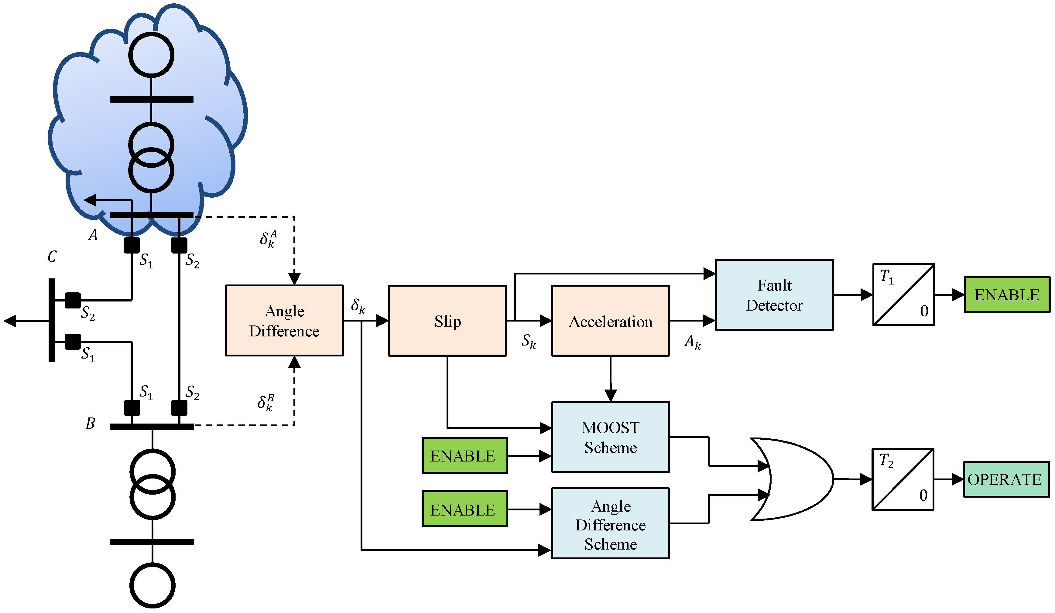
Figure 3 shows the proposed ASS for LPS based on a WAMPC. The control scheme detects possible instability situations based on a combination of a modified OOST and the angle difference method. As can be seen, the scheme first measures the PSV angle at two network buses (
and
) and then calculates its angular difference
. Based on this, the first and second derivatives are obtained to get the slip frequency
and the acceleration
, respectively. To avoid misoperations of the ASS, the MOOST and angle difference elements are only enabled after a set time delay
. To accomplish this, a fault detector element is also included. This element compares the absolute value of the slip frequency
and the acceleration
with suitable thresholds (
and
, respectively). Equations (
11) and (
12) define the conditions when a fault is detected.
When either Equation (
11) or (
12) is fulfilled for a time
, the MOOST and angle difference elements begin to check the current operating region of the system based on the limits defined in
Figure 2 and Equation (
4), respectively. If at least one of the conditions established in Equations (
4), and (
7)–(
10) is satisfied for a predefined time
, an unstable condition has been detected and the ASS starts to operate. Otherwise, the ASS remains blocked. In the illustrative network shown in
Figure 3, the line switches
and
in the bus
A are opened if the scheme operates.
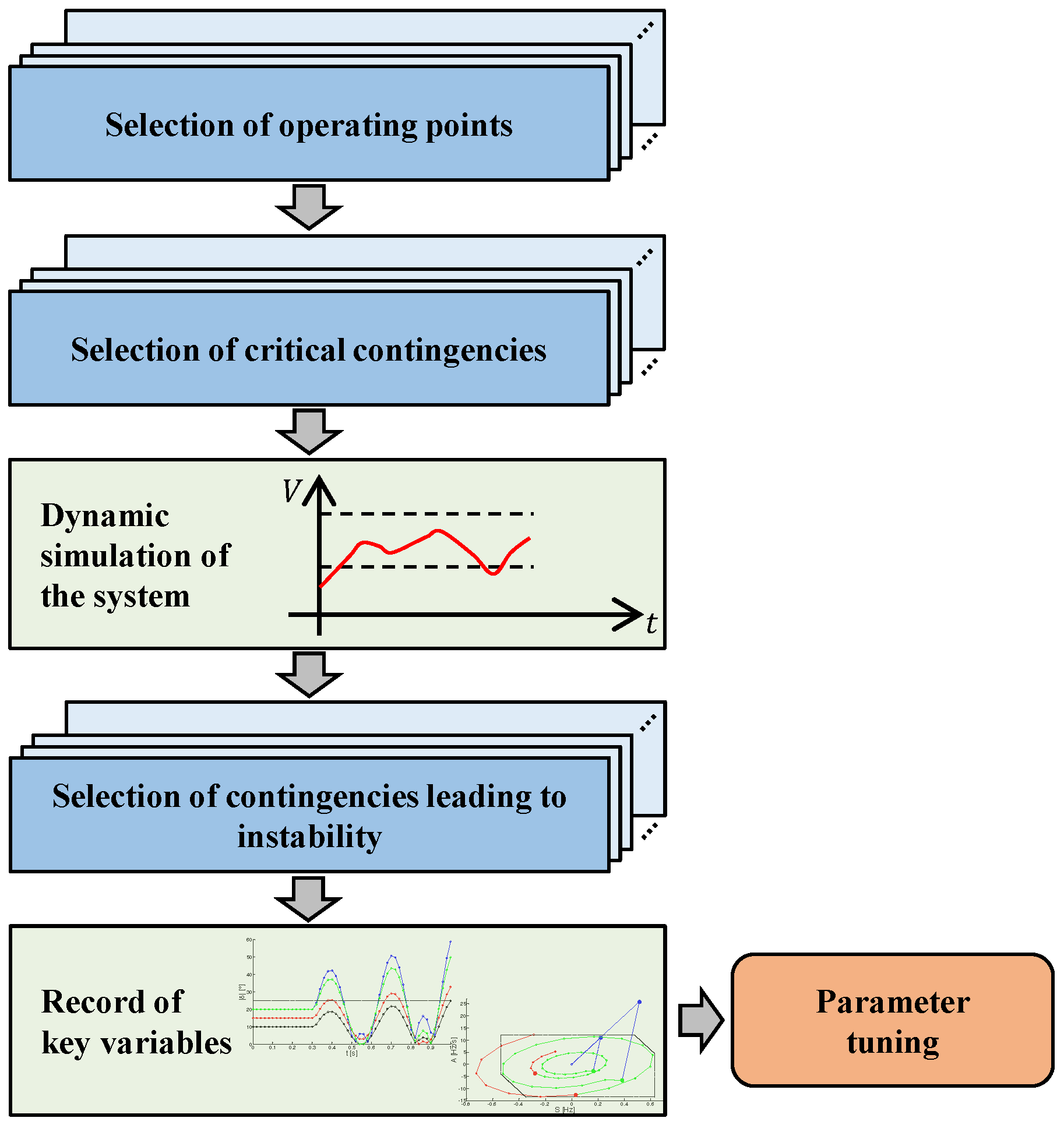
4.2. Parameter Tuning
As usual in OOST and angle difference elements, the parameters of the control scheme must be set according to the technical characteristics of each power system. This process must be performed based on detailed dynamic models of the system under study and considering a wide set of scenarios.
Figure 4 shows the proposed block diagram of the methodology for tuning the parameters needed in the proposed ASS.
The first steps of the methodology are to select a sound set of operating points and critical contingencies. In dynamic assessments of real power systems, the simulations are performed only for some critical contingencies and operating points of the system (worst-case scenario). This approach is justified since the dynamic analysis of all possible contingencies and operating conditions of a real power system would lead to an impractical amount of time and simulations.
The operating points to be considered in the tuning process must be able to properly represent critical conditions that the system may experience from a stability perspective. LPS are characterized by weak longitudinal structures with radial configuration, long transmission lines, and generation centers electrically remote from load centers [
1,
2,
3]. Consequently, high power transfers over their long transmission lines, as well as highly loaded conditions in generators are typically critical operating conditions of these power systems [
33]. Thus, operating points that reflect these conditions are recommended to be included in the tuning process. Furthermore, operating points identified as critical by TSOs should also be included.
Once the set of operating points are properly defined, the next step is to select a set of critical contingencies for each selected operating point. Two-phase to ground short circuits at high loaded transmission lines (with its pertinent disconnection for fault clearing) are generally considered as credible and also critical faults [
33]. The sudden outage of highly loaded generators may also be considered. Especially in LPS, the selection should also include the knowledge of TSOs and the records of real blackouts in the system. TSOs of LPS know those cases in which traditional remedial actions will not be able to save the system from a total blackout. In those circumstances, splitting the system in different islands is the only remedial action to avoid the total system collapse. Alternatively, a mathematical algorithm for the selection of critical contingencies is proposed in [
34]. In this work, the authors propose a screening and ranking method for transient stability assessments based on the modal synchronizing torque coefficient of the synchronous machines, which is computed by eigenvalue sensitivity analysis. Additional to the aforementioned work, Arrieta et al. [
35], Baone et al. [
36], and Wang et al. [
37], also proposed contingency rankings based on eigenvalue analysis.
The next step of the methodology is to simulate, for each operating point, the selected set of contingencies using time-domain dynamic simulations. If a contingency leads to system instability, it must be selected and then considered to set the value of the parameters of the ASS. For those contingencies leading to system instability, three key variables must be recorded: the angular difference, slip frequency and acceleration at the defined measurements points.
As shown in
Figure 3, three main components of the ASS need a parameter tuning process: angle difference scheme, the MOOST scheme and the fault detector element. The following sections give details on this regard.
4.2.1. Angle Difference Scheme
The first parameter to be defined is the maximum threshold
of the angle difference scheme (see Equation (
4)). Considering the set of contingencies leading to system collapse,
can be obtained according to:
where the subindices
i and
j represent the operating point (OP) and the contingency, respectively.
is the angle difference in steady state considering the OP
i. To avoid misoperations of the scheme during normal operation,
has to be greater than all
under consideration.
Figure 5 and
Table 2 show illustratively how the angle difference scheme tuning is carried out. In this example, two critical contingencies (CC) leading the system towards its collapse are analyzed considering three different operating points.
Figure 5 depicts how the absolute difference angle
(see Equation (
3)) evolves between two buses of the system and
Table 2 shows the initial angle
and
for each OP and CC. In these cases, the disturbance occurs at
, and depending on the OP and contingency, the system could reach a point in which it is no longer able to maintain its stability. This point is represented as
in
Table 2. Considering Equation (
13) and the values shown in
Table 2, the maximum angular difference threshold
is defined as
.
4.2.2. MOOST Scheme
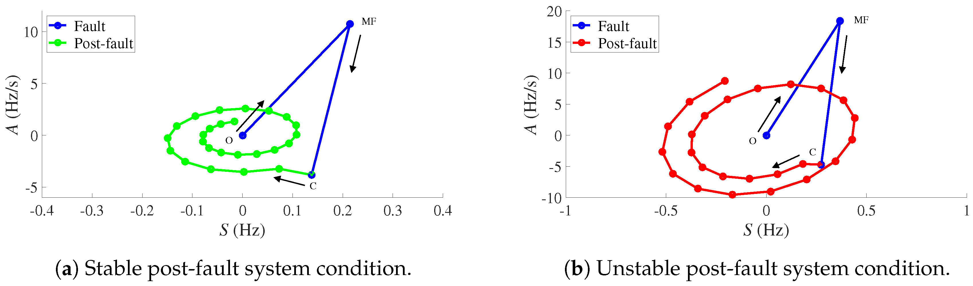
To establish the parameters for the MOOST scheme it is necessary to identify three key points of the
trajectories during a contingency: (1) steady state condition; (2) fault condition; and (3) post-fault condition.
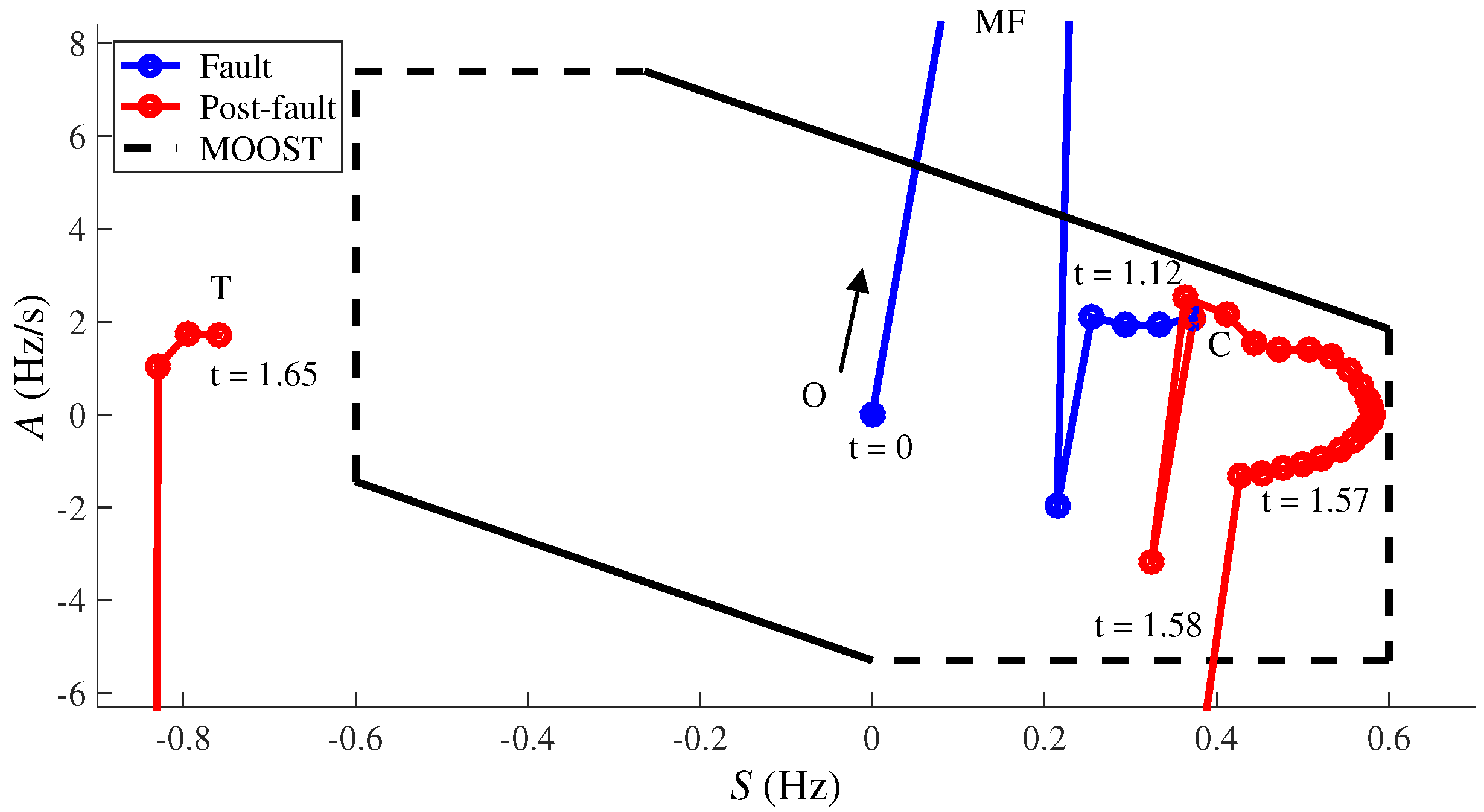
Figure 6 illustrates this process for an (a) stable and (b) unstable post-fault system condition. The initial point of the blue trajectory, points
O in
Figure 6, represents the steady state condition (stable). Once the fault is applied, the trajectory moves towards a maximum value indicated as
in
Figure 6. When the fault is cleared, the trajectory
moves to point
C. If the system is stable, the trajectory
will finally converge into the origin during the post-fault condition as shown in
Figure 6a. Otherwise, the trajectory will follow a divergent spiral trajectory from the origin, indicating an unstable condition
Figure 6b.
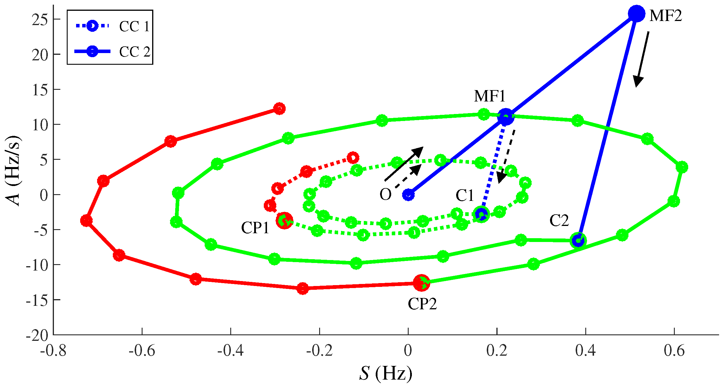
During unstable post-fault conditions, there is a point (critical point
) from which the system is no longer able to maintain its stability if no extreme corrective actions are taken. At this point, system blackout is imminent, and the MOOST scheme should operate to separate the affected areas aiming to avoid the total system collapse. To illustrate this point, let consider the two trajectories (representing the system evolution) for two different contingencies shown in
Figure 7. Dashed and solid arrows indicate the trajectory followed by the system in the first and the second contingency, respectively. In this example, both trajectories are divided into three parts. The blue section of the trajectories represents the evolution of the system during the fault; with a maximum value (during the fault) highlighted as
and
. The green section of the trajectories starts with the fault clearance (
and
in
Figure 7). These points are characterized by a network condition in which the system could still sustain its stability if sound remedial actions are taken. Finally, the red sections start at the critical points
and
from which the system collapse is imminent.
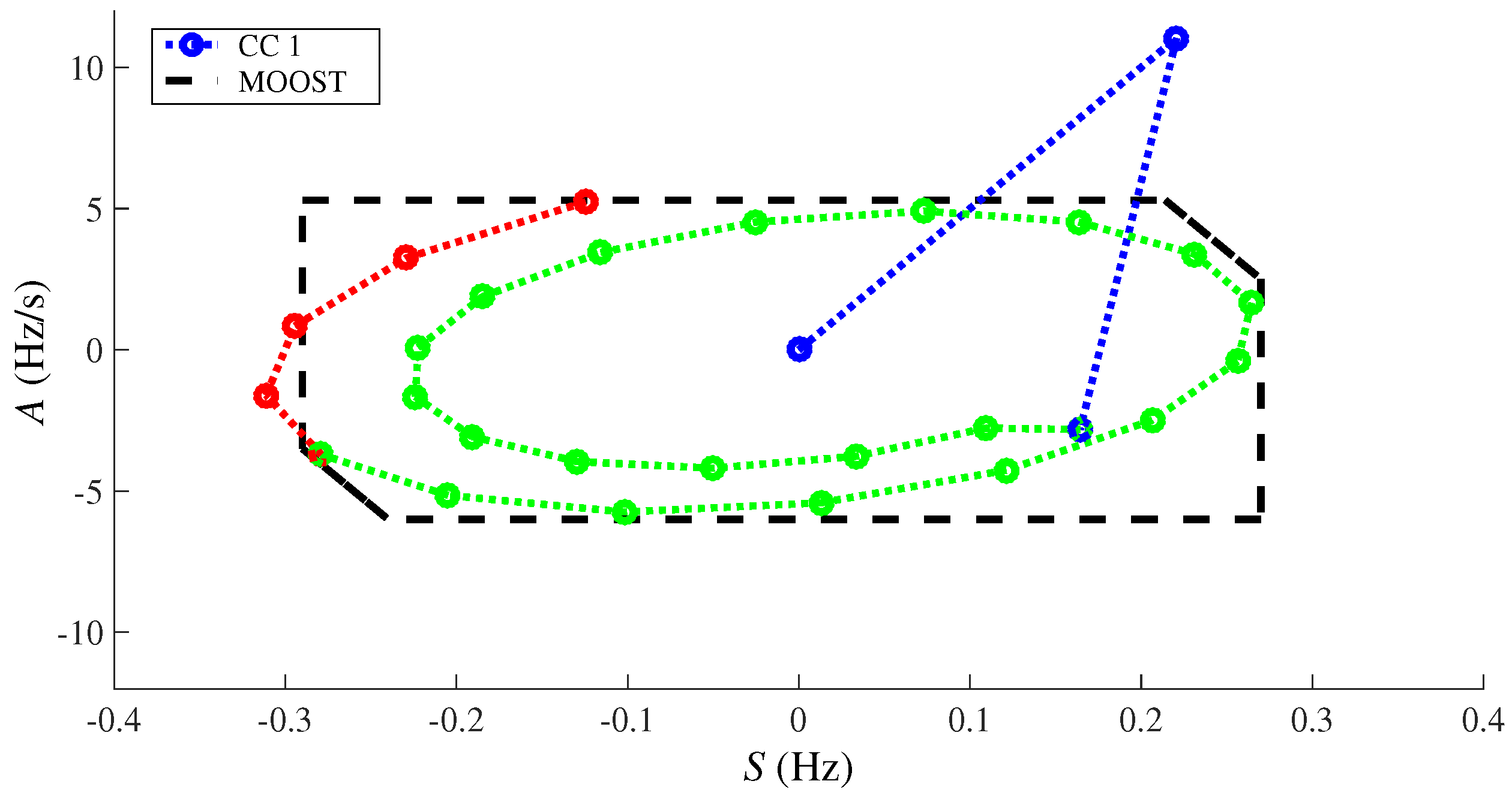
On the assumption that there is no other remedial action to avoid the collapse of the system, the MOOST scheme should operate either if CC 1 or CC 2 occurs. Therefore, the green section of the minimum trajectory must be limited (in this example: CC 1). One way to accomplish this is by setting the parameters of the scheme graphically (see
Figure 8).
The first step is to identify the limiting points in each direction of the stable trajectory (
E,
F,
G and
H in
Figure 8). Each of these points can be directly associate to the parameters
,
,
and
of the MOOST scheme. Then, by extending a line from either
F or
H to the y-axis (
), the offset
or
can be obtained as the y-intercept. When
or
is set, the parameter
K can be calculated by the slope between two points. Finally, the remaining offset can be obtained by the classical equation for non-vertical lines.
Table 3 shows the parameters obtained by following these steps and
Figure 9 shows the resulting MOOST normal operation region.
4.2.3. Fault Detector
Several fault detection approaches, such as wavelet transform, neural network and statistical techniques, have been presented in the literature [
38]. Since the scope of this work is to avoid the total collapse of the system during “well known” critical contingencies, a deterministic way to detect the faults is proposed. The fault detector element must enable both, the angle difference and the MOOST schemes during the selected contingencies. By choosing the minimum absolute value of
(obtained from the set of critical contingencies leading to the system collapse), the thresholds needed in the fault detector element (
and
) must be selected according to:
where
is the acceleration and
the slip frequency, both at the
point. Subindices
i and
j represent the operating point and the contingency, respectively. This guarantees that the angle difference and the MOOST schemes will be enabled for all the contingencies leading to system collapse.
Although in this work the thresholds in the fault detector are defined in a deterministic way, the methodology can also be applied considering statistical approaches such as [
39].
4.3. Considerations and Practical Implementation
To implement the proposed ASS, it is necessary to identify suitable areas to be saved when a critical contingency occurs. The selected areas to be saved should meet at least the following requirements:
The area must have an adequate reserve of active and reactive power to meet the load demand [
31].
The network constraints and systems limits must be satisfied (thermal capacity on transmission lines and transformers, frequency and bus voltages at prescribed values, among others [
28,
40]).
Once the candidates to island regions are identified either by TSO knowledge or by other strategy such as the ones proposed in [
28,
40], the measurement points to be used as input for the ASS must be determined. In real power systems, controlled splitting is often restricted to tie-lines which naturally divide the network into islands, even more if the network has a longitudinal structure [
41]. Therefore, if the area selected is interconnected to the main power system by one tie-line, the PMUs should be installed on both sides of the separation interface [
41,
42]. Moreover, chosen these points will be useful to monitor the restoration progress and the readiness for resynchronization [
42]. Besides, if the selected area is interconnected by more than a link, three options are recommended:
Electrical centers: The natural separation of a system begins at the electrical centers [
43]. Therefore, these points may be suitable to install the PMUs.
At major generation points: As generators have a significant role on system stability, selecting to install the PMUs is more appropriate [
44].
Major centers of inertia: In both sides of the boundary, where the boundary is defined as a constraint when composite angle is used to represent each area [
45].
It is also recommended to prioritize measurement points with higher voltage levels [
42].
To implement the proposed scheme, the following infrastructure/equipment is required:
Two PMUs and GPS clocks to measure the phase angles of the PSV with a time reference.
One phasor data concentrator (PDC) and GPS clock to align the data and make it coherent to logic.
One central computer to implement the ASS algorithm.
Communication infrastructure.
It is worth noting that the MRATE of the PMUs determines the best case timing for detecting a change that may require protection action [
46]. Nowadays, almost every commercially available device allows to choose a MRATE between a given range (1 to 120 phasors per second). The selection will depend on the purpose, the available communication and information storage infrastructure, system’s frequency, among others. Therefore, choosing a device with a higher reporting rate would improve the performance of the proposed scheme. However, this may also increase the costs since a better communication and information storage infrastructure will be required.
5. Case Study
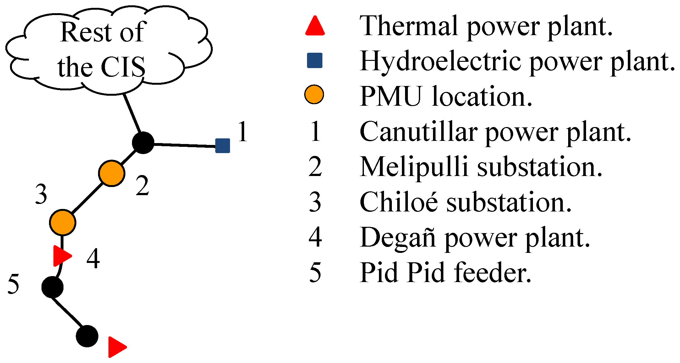
The simulations were based on the CIS of Chile. In order to illustrate the structure of the network, a simplified diagram is shown in
Figure 10. The CIS is a good example of extreme LPS; it has long transmission lines covering a total length of near 2300 km. The CIS supplies a peak load of 7300 MW with the major load located in Santiago, Chile’s capital, placed in the central part of the system and encompassing around one third of the country’s population. The system is mainly composed by thermal and hydroelectric power stations. Hydroelectric power plants are mostly concentrated in the south of the CIS comprising near the 50% of the whole installed capacity. Due to the structure of the CIS, different areas may be adequate to evaluate the performance of the proposed scheme. According to Chilean TSOs experience, one area which could be saved when a blackout in the system is imminent is Chiloé Island. The island is located at the end of the CIS and is interconnected by a single 220 kV line. The zone to be split and the PMUs location are shown in
Figure 10. Although from a topology perspective the Chilean network may be categorized as a simple problem, this system is especially interesting from a stability perspective due to its extreme longitudinal structure and characteristics. Indeed, several works confirm that the Chilean system is prone to face stability problems in cases in which meshed networks would not [
17,
47].
The study was conducted for three operating points namely OP1, OP2, and OP3, which are characterized by high power transfers through the 500 kV corridor Charrúa-Ancoa of near 180 km long (marked as “3” in
Figure 10). The power transfer through the corridor is 1000 MW for all OPs under study.
Table 4 shows the generation and demand for each OP.
6. Results
The CIS network model used in this study contained approximately 12,500 buses and 600 demand points distributed throughout the network. The study was performed with the simulation tool DIgSILENT PowerFactory and a MRATE of 50 messages per second for each PMUs was used.
6.1. Critical Contingency
To tune the parameters of the proposed ASS, a two-phase to ground short circuit in one circuit of the line Charrúa-Ancoa was selected as critical contingency. The contingency was chosen based on the knowledge and experience of Chilean TSOs [
48,
49]. The fault is cleared after
through the disconnection of the pertinent circuit. Because of an erroneous operation of the protection scheme, the remaining circuit is also disconnected after
. The disconnection of the corridor Charrúa-Ancoa splits the CIS into two unstable islands: the Central-North island (covering from substation Ancoa to the north) and the South island (from substation Charrúa to the south). According to the Chilean TSOs, in most cases this contingency leads to a total blackout of the CIS [
48,
49].
6.2. Proposed Active Splitting Scheme
The simulation of the CC was used to tune the parameters as explained in
Section 4.2. The results are shown in
Table 5.
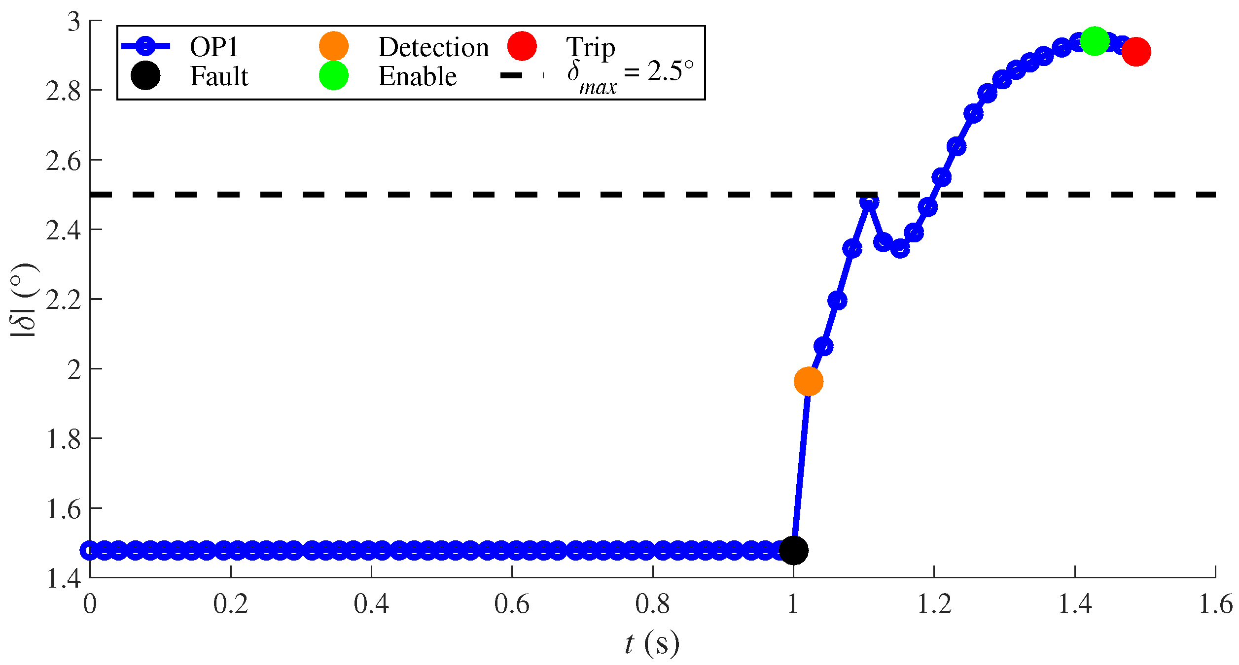
Figure 11 shows the evolution of the absolute angle difference calculated by the proposed scheme during the contingency when considering the operating point OP1. The fault begins at
(black point in the figure) and is detected by the fault detector element at
(yellow point). After
from the fault detection, the angle difference and the MOOST schemes are enabled (green point). When
reaches the threshold
and the time
is fulfilled, the scheme starts to operate by splitting Chiloé Island from the CIS.
Figure 12 shows the trajectory in the
plane for the OP2. The
trajectory starts around the origin (point
O) which represent the steady state condition before the fault appliance (
). The fault condition is represented as a blue trajectory on the figure. After
the fault is cleared (point
C) and the post-fault trajectory (red line in the figure), remains inside the MOOST region for
. At
, the trajectory leaves the stable region in the
plane, thus triggering the MOOST element due to
boundary. The element trips when the timer
is satisfied (point
T), allowing the splitting of Chiloé Island from the CIS.
Table 6 summarizes the operation of each element of the proposed ASS. As can be seen, the fault detector element detects the contingency for all OPs, allowing the activation of the angle difference and the MOOST element. While both schemes triggered at the same time for the operating point OP1, the MOOST element triggered at the first place for OP2 and OP3. Moreover, the MOOST element was activated due to the satisfaction of the new restrictions (Equations (
9) and (
10)), allowing to detect the unstable operating point before the trajectory
leaves the stable region through the boundaries defined in Equations (
7) and (
8). Therefore, with the proposed scheme, it is possible to take faster remedial actions than with a traditional OOST element (Equations (
7) and (
8)), gaining valuable time at the moment of the splitting.
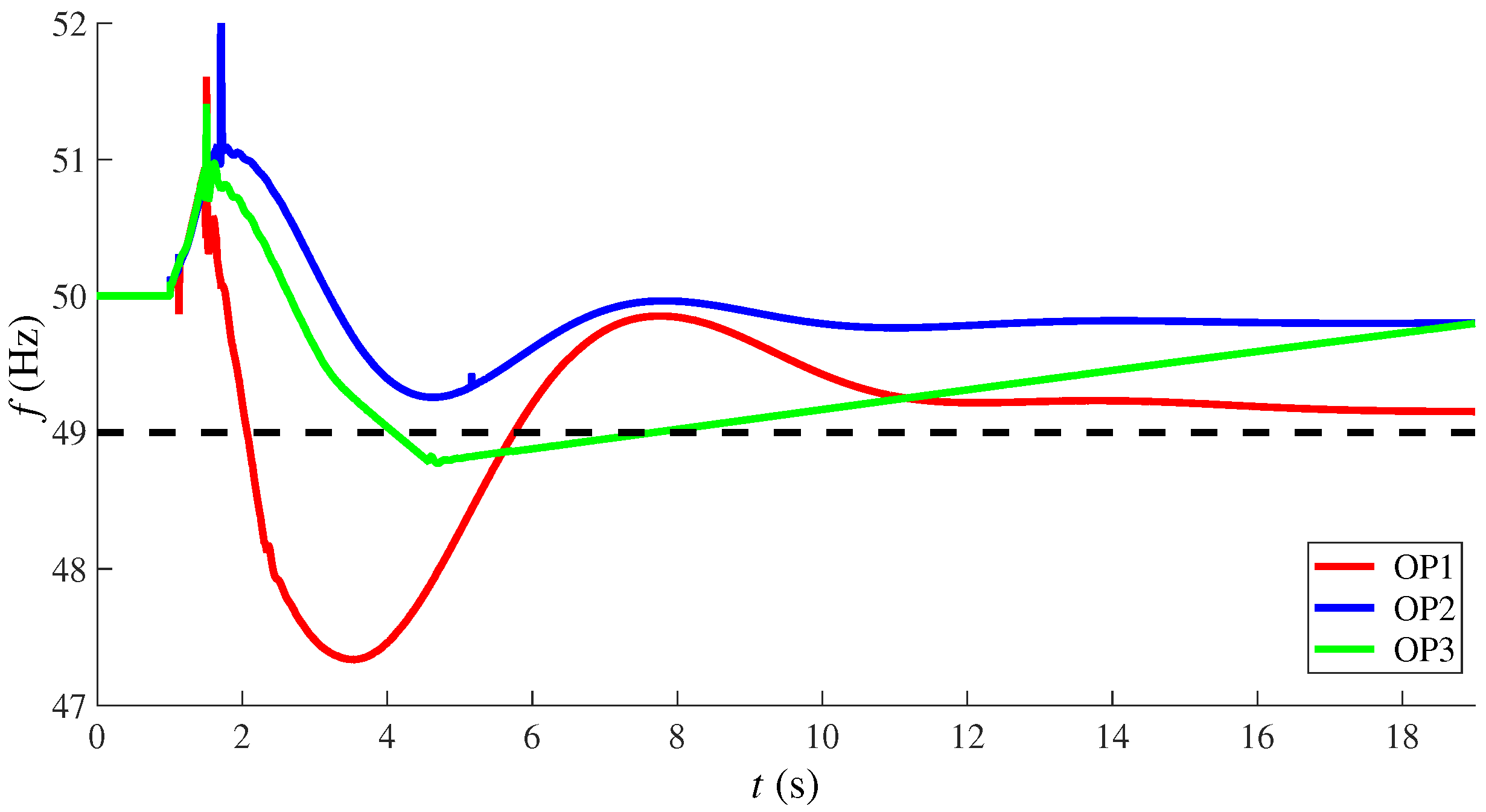
After the splitting, Chiloé Island remained stable for two of the three operating points (OP1 and OP2). After
from the operation of the ASS scheme, the frequency of the island (shown in
Figure 13) reflects the existing power balance between generation and load for the operating points OP1 and OP2. In OP3, all generator units of Chiloé Island loss synchronism. This is reflected in the continuous increase of the frequency during the simulation.
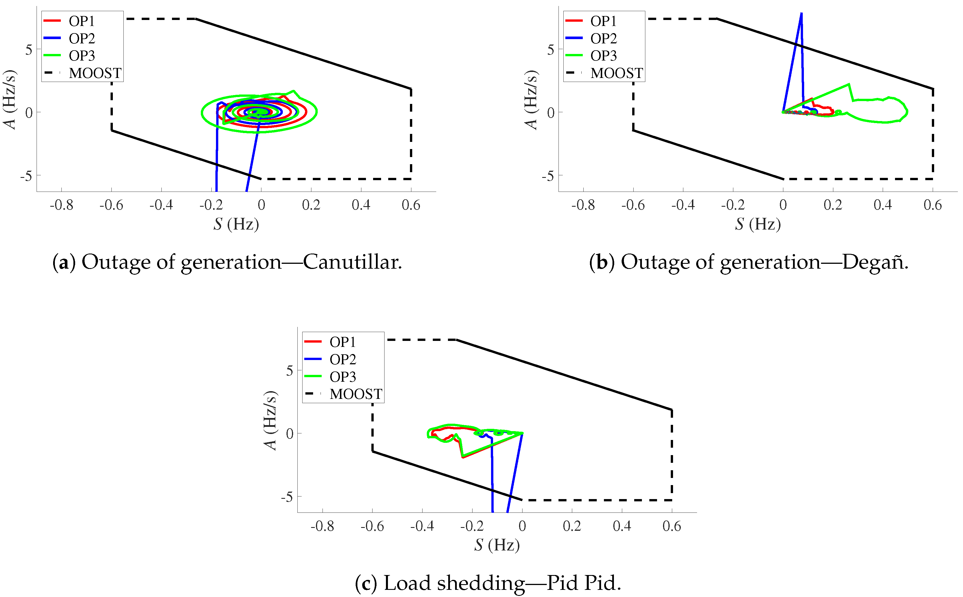
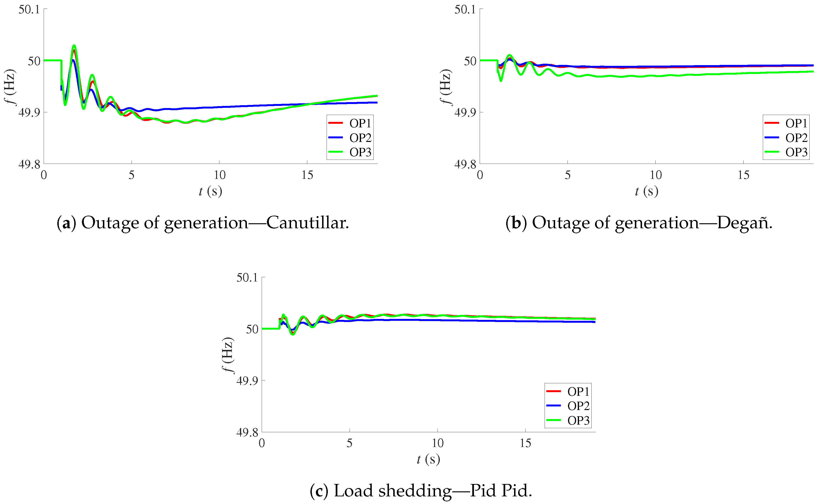
6.3. Performance of the Proposed Active Splitting Scheme Under Different Contingencies
The following subsection shows the performance of the proposed ASS under three different contingencies: outage of generation outside Chiloé Island (Canutillar power plant), outage of generation inside Chiloé Island (Degañ power plant) and load shedding inside Chiloé Island (Pid Pid feeder). The aforementioned points are shown in
Figure 14 and the detailed outage of generation/load shedding is shown in
Table 7.
The ASS’s response was the same for each contingency. The fault detector element enabled both the MOOST and the angle difference scheme after the fault appliance. However, since no condition established in Equations (
4), and (
7)–(
10) was satisfied for the predefined time
, the ASS did not operate. Therefore, no splitting took place.
Table 8 summarizes the aforementioned behavior.
Figure 15 shows the
trajectory for each operating point and contingency. It can be seen that after the fault appliance every trajectory converges into the origin, without triggering the MOOST scheme.
The network frequency for each case is shown in
Figure 16. It can be seen that the performance of the proposed scheme was satisfactory for all three contingencies.
7. Conclusions
This paper proposed an active splitting control scheme especially suitable for LPS based on a WAMPC using synchrophasor measurements. The proposed control scheme detects possible instability situations by means of a modified OOS algorithm combined with the angle difference method. The proposal is a last remedial action to save some pre-identified areas when a total system blackout is imminent.
The simulation results indicated that the angle difference element could operate before or at the same time than an out-of-step element, making a more reliable protection scheme. Furthermore, with the modified OOST scheme, it is possible to take faster remedial actions than with a traditional OOST element if upper and lower boundaries of the slip frequency and acceleration are used. Since phase angles in a LPS may change drastically even when small changes in active power occur, these limits may accelerate the prediction of system instabilities and thus gain valuable time at the moment of the splitting. Finally, the results also shown that the proposed fault detector element, based on the first and second derivative of the angle difference measurement between two buses, could be useful for detecting several disturbances in a LPS.
As future work, it is proposed to evaluate the time-response of the scheme when the latencies in measurements, communication and processing are considered. For instance, since each individual PMU may have different latencies, the ASS design should account for this in order to determine if the selected equipment can actually achieve the desired protection scheme performance.
Another interesting work would be to extend the methodology when several schemes are proposed—at multiple locations throughout the network—to split the system into different parts. The operation of each scheme in a separated way (isolated) and also in a coordinated one should be considered.
Finally, extending the proposed methodology to cover more complex power systems such as meshed ones will be a motivating challenge too.
Acknowledgments
The authors acknowledge the support of Tecma S.A. and Schweitzer Engineering Laboratories, Inc. in the realization of this work. This research was partially funded by the Complex Engineering Systems Institute, ISCI (ICM-FIC: P05-004-F, CONICYT: FB0816).
Author Contributions
Felipe Arraño-Vargas designed the scheme, and performed the model simulations and analysis; Felipe Arraño-Vargas and Claudia Rahmann designed the parameter tuning methodology; Claudia Rahmann and Felipe Valencia contributed materials, and performed the continuous follow-up of the study; Luis Vargas performed the supervision and provided professional advice.
Conflicts of Interest
The authors declare no conflict of interest.
References
- Aboytes, F.; Arroyo, G. Security Assessment in the Operation of Longitudinal Power Systems. IEEE Trans. Power Syst. 1986, PWRS-1, 225–232. [Google Scholar] [CrossRef]
- Chakrabarti, A.; Mukhopadhyay, A.K. Operating Problems in Longitudinal Power Supply Systems. In Proceedings of the 4th IEEE Region 10 International Conference TENCON ’89, Bombay, India, 22–24 November 1989; pp. 932–935. [Google Scholar]
- Aboytes, F.; Arroyo, G.; Villa, G. Application of Static Var Compensators in Longitudinal Power Systems. IEEE Trans. Power Appar. Syst. 1983, PAS-102, 3460–3466. [Google Scholar] [CrossRef]
- North American Electric Reliability Corporation (NERC). Real-Time Application of Synchrophasors for Improving Reliability; NERC: Atlanta, GA, USA, 2010. [Google Scholar]
- Čerina, Z.; Šturlić, I.; Matica, R.; Skendžić, V. Synchrophasor Applications in the Croatian Power System. In Proceedings of the 36th Annual Western Protective Relay Conference, Spokane, WA, USA, 20–22 October 2009; pp. 1–7. [Google Scholar]
- Begovic, M.; Novosel, D.; Karlsson, D.; Henville, C.; Michel, G. Wide-Area Protection and Emergency Control. Proc. IEEE 2005, 93, 876–891. [Google Scholar] [CrossRef]
- Fischer, N.; Benmouyal, G.; Hou, D.; Tziouvaras, D.; Byrne-Finley, J.; Smyth, B. Tutorial on Power Swing Blocking and Out-of-Step Tripping. In Proceedings of the 39th Annual Western Protective Relay Conference, Spokane, WA, USA, 16–18 October 2012; pp. 1–20. [Google Scholar]
- Tziouvaras, D.A.; Hou, D. Out-of-Step Protection Fundamentals and Advancements. In Proceedings of the 57th Annual Conference for Protective Relay Engineers, College Station, TX, USA, 30 March–1 April 2004; pp. 282–307. [Google Scholar]
- Franco, R.; Sena, C.; Taranto, G.N.; Giusto, A. Using Synchrophasors for Controlled Islanding—A Prospective Application for the Uruguayan Power System. IEEE Trans. Power Syst. 2013, 28, 2016–2024. [Google Scholar] [CrossRef]
- Vargas, L.; Huber, E.; Palma-Behnke, R. System Security and Dynamic Performance in the Chilean Central Interconnected System. In Proceedings of the IEEE Power Systems Conference and Exposition, Atlanta, GA, USA, 29 October–1 November 2006; pp. 406–408. [Google Scholar]
- Brokering, W.; Palma, R.; Vargas, L. Los Sistemas Eléctricos de Potencia, 1st ed.; Pearson Educación de México S.A. de C.V.: Naucalpan de Juárez, Mexico, 2008. [Google Scholar]
- Stott, B.; Alsac, O. Fast Decoupled Load Flow. IEEE Trans. Power Appar. Syst. 1974, PSA-93, 859–869. [Google Scholar] [CrossRef]
- Doan, V.D.; Tseng, T.H.; Huang, P.H. Effects of Power System Stabilizer on inter-area Oscillation in a Longitudinal Power System. In Proceedings of the 10th International Power & Energy Conference (IPEC), Ho Chi Minh City, Vietnam, 12–14 December 2012; pp. 455–460. [Google Scholar]
- Chang, C.L.; Liu, C.S.; Ko, C.K. Experience with power system stabilizers in a longitudinal power system. IEEE Trans. Power Syst. 1995, 10, 539–545. [Google Scholar] [CrossRef]
- Román Messina, A.; Ramírez, J.M.; Cañedo C., J.M. An Investigation on the use of Power System Stabilizers for Damping Inter-Area Oscillations in Longitudinal Power Systems. IEEE Trans. Power Syst. 1998, 13, 552–559. [Google Scholar] [CrossRef]
- Hsu, Y.Y.; Shyue, S.W.; Su, C.C. Low Frequency Oscillations in Longitudinal Power Systems: Experience with Dynamic Stability of Taiwan Power System. IEEE Power Eng. Rev. 1987, PER-7, 35. [Google Scholar] [CrossRef]
- Vargas, L.; Quintana, V.; Miranda, R. Voltage Collapse Scenario in the Chilean Interconnected System. IEEE Trans. Power Syst. 1999, 14, 1415–1421. [Google Scholar] [CrossRef]
- Hain, Y.; Schweitzer, I. Analysis of the Power Blackout of June 8, 1995 in the Israel Electric Corporation. IEEE Trans. Power Syst. 1997, 12, 1752–1758. [Google Scholar] [CrossRef]
- O’Keefe, R.J.; Schulz, R.P.; Bhatt, F.B. Improved Representation of Generator and Load Dynamics in the Study of Voltage Limited Power System Operations. IEEE Trans. Power Syst. 1997, 12, 304–314. [Google Scholar] [CrossRef]
- Kosterev, N.V.; Yanovsky, V.P.; Kosterev, D.N. Modeling of Out-of-Step Conditions in Power Systems. IEEE Trans. Power Syst. 1996, 11, 839–844. [Google Scholar] [CrossRef]
- Bonanomi, P. Phase Angle Measurements with Synchronized Clocks-Principle and Applications. IEEE Trans. Power Appar. Syst. 1981, PAS-100, 5036–5043. [Google Scholar] [CrossRef]
- IEEE Power System Relaying Committee. Power Swing and Out-of-Step Considerations on Transmission Lines; IEEE PES-PSRC: Calgary, Alberta, Canada, 2005. [Google Scholar]
- Guzmán-Casillas, A. Systems and Methods for Power Swing and Out-of-Step Detection using Time Stamped Data. U.S. Patent No. 7,930,117, 19 April 2011. [Google Scholar]
- Mulhausen, J.; Schaefer, J.; Mynam, M.; Guzmán, A.; Donolo, M. Anti-Islanding Today, Successful Islanding in the Future. In Proceedings of the 63rd Annual Conference for Protective Relay Engineers, College Station, TX, USA, 29 March–1 April 2010; pp. 1–8. [Google Scholar]
- Guzmán, A.; Mynam, V.; Zweigle, G. Backup Transmission Line Protection for Ground Faults and Power Swing Detection Using Synchrophasors. In Proceedings of the 34th Annual Western Protective Relay Conference, Spokane, WA, USA, 16–18 October 2007; pp. 1–11. [Google Scholar]
- Quirós-Tortós, J.; Sánchez-García, R.; Brodzki, J.; Bialek, J.; Terzija, V. Constrained Spectral Clustering Based Methodology for Intentional Controlled Islanding of Large-Scale Power Systems. IET Gener. Transm. Distrib. 2015, 9, 31–42. [Google Scholar] [CrossRef]
- Jiang, T.; Jia, H.; Yuan, H.; Zhou, N.; Li, F. Projection Pursuit: A General Methodology of Wide-Area Coherency Detection in Bulk Power Grid. IEEE Trans. Power Syst. 2016, 31, 2776–2786. [Google Scholar] [CrossRef]
- Zhao, Q.; Sun, K.; Zheng, D.-Z.; Ma, J.; Lu, Q. A Study of System Splitting Strategies for Island Operation of Power System: A Two-Phase Method Based on OBDDs. IEEE Trans. Power Syst. 2003, 18, 1556–1565. [Google Scholar] [CrossRef]
- Australian Energy Regulator (AER). The Events of 16 January 2007 Investigation Report; AER: Melbourne, Australia, 2007.
- Power System Operator of Chile (CDEC). Estudio Para Análisis de Falla EAF 091/2016: Desconexión Forzada Transformador N°6 225/161/69 kV S/E Alto Jahuel; CDEC: Santiago, Chile, 2016. [Google Scholar]
- Kundur, P. Power System Stability and Control, 1st ed.; McGraw-Hill, Inc.: New York, NY, USA, 1994. [Google Scholar]
- Arraño, F. Esquema de Detención de Inestabilidad para Operación en Isla Eléctrica Utilizando Sincrofasores. Bachelor’s Thesis, Universidad de Chile, Santiago, Chile, 2014. [Google Scholar]
- Savulescu, S.C. Real-Time Stability Assessment in Modern Power System Control Centers; John Wiley & Sons, Ltd.: Hoboken, NJ, USA, 2009. [Google Scholar]
- Nam, H.K.; Shim, K.S.; Kim, Y.K.; Song, S.G.; Lee, K.Y. Contingency Ranking for Transient Stability via Eigen-Sensitivity Analysis of Small Signal Stability Model. In Proceedings of the EEE Power Engineering Society Winter Meeting, Singapore, 23–27 January 2000; Volume 2, pp. 861–865. [Google Scholar]
- Arrieta, R.; Ríos, M.A.; Torres, A. Contingency Analysis and Risk Assessment of Small Signal Instability. In Proceedings of the IEEE Lausanne Power Tech, Lausanne, Switzerland, 1–5 July 2007; pp. 1741–1746. [Google Scholar]
- Baone, C.A.; Acharya, N.; Veda, S.; Chaudhuri, N.R. Fast Contingency Screening and Ranking for Small Signal Stability Assessment. In Proceedings of the IEEE PES General Meeting | Conference & Exposition, National Harbor, MD, USA, 27–31 July 2014; pp. 1–5. [Google Scholar]
- Wang, Z.; Gan, D.; Chung, C.Y.; Wong, K.P.; Shen, C. Robust PSS Design Considering Power System Contingencies Based on a Recursive PSO. In Proceedings of the 8th World Congress on Intelligent Control and Automation (WCICA), Jinan, China, 7–9 July 2010; pp. 668–675. [Google Scholar]
- Bunnoon, P. Fault Detection Approaches to Power System: State-of-the-Art Article Reviews for Searching a New Approach in the Future. Int. J. Electr. Comput. Eng. (IJECE) 2013, 3, 553–560. [Google Scholar] [CrossRef]
- Gilbert, D.M.; Morrison, I.F. A statistical method for the detection of power system faults. In Proceedings of the IPST’95—International Conference on Power systems Transients, Lisbon, Portugal, 3–7 September 1995; pp. 288–293. [Google Scholar]
- Trodden, P.A.; Bukhsh, W.A.; Grothey, A.; McKinnon, K.I.M. Optimization-Based Islanding of Power Networks Using Piecewise Linear AC Power Flow. IEEE Trans. Power Syst. 2014, 29, 1212–1220. [Google Scholar] [CrossRef]
- Machowski, J.; Bialek, J.; Bumby, J. Power System Dynamics: Stability and Control, 2nd ed.; John Wiley & Sons, Ltd.: Chichester, West Sussex, UK, 2010. [Google Scholar]
- North American SynchroPhasor Initiative (NASPI). Guidelines for Siting Phasor Measurement Units. Available online: http://www.naspi.org/node/405 (accessed on 26 December 2017).
- Soman, S.A.; Nguyen, T.B.; Pai, M.A.; Vaidyanathan, R. Analysis of Angle Stability Problems: A Transmission Protection Systems Perspective. IEEE Trans. Power Deliv. 2004, 19, 1024–1033. [Google Scholar] [CrossRef]
- Wu, Y.; Musavi, M.; Lerley, P. Synchrophasor-Based Monitoring of Critical Generator Buses for Transient Stability. IEEE Trans. Power Syst. 2016, 31, 287–295. [Google Scholar] [CrossRef]
- North American Electric Reliability Corporation (NERC). Reliability Guideline: PMU Placement and Installation; NERC: Atlanta, GA, USA, 2016. [Google Scholar]
- O’Brien, J.; Deronja, A.; Apostolov, A.; Arana, A.; Begovic, M.; Brahma, S.; Brunello, G.; Calero, F.; Faulk, H.; Hu, Y.; et al. Use of Synchrophasor Measurements in Protective Relaying Applications. In Proceedings of the 67th Annual Conference for Protective Relay Engineers, College Station, TX, USA, 30 March–1 April 2014; pp. 23–29. [Google Scholar]
- Vargas, L.; Cañizares, C. Time Dependence of Controls to Avoid Voltage Collapse. IEEE Trans. Power Syst. 2000, 15, 1367–1375. [Google Scholar] [CrossRef]
- Power System Operator of Chile (CDEC). Revisión del Plan de Defensa contra Contingencias Extremas; CDEC: Santiago, Chile, 2013. [Google Scholar]
- Estudios Eléctricos (EE). Estudio de Detalle Para PDCE Charrúa—Ancoa; EE: Rosario, Argentina, 2011. [Google Scholar]
Figure 1.
Out-of-step tripping (OOST) characteristic in the plane.
Figure 1.
Out-of-step tripping (OOST) characteristic in the plane.
Figure 2.
Modified OOST (MOOST) characteristic in the plane.
Figure 2.
Modified OOST (MOOST) characteristic in the plane.
Figure 3.
Active splitting scheme (ASS) for longitudinal power system (LPS) based on a wide-area monitoring, protection and control (WAMPC).
Figure 3.
Active splitting scheme (ASS) for longitudinal power system (LPS) based on a wide-area monitoring, protection and control (WAMPC).
Figure 4.
Flowchart of the methodology for parameter tuning.
Figure 4.
Flowchart of the methodology for parameter tuning.
Figure 5.
Tuning of the angle difference scheme.
Figure 5.
Tuning of the angle difference scheme.
Figure 6.
trajectories.
Figure 6.
trajectories.
Figure 7.
trajectories for contingencies CC 1 and CC 2.
Figure 7.
trajectories for contingencies CC 1 and CC 2.
Figure 8.
Illustrative tuning of the MOOST scheme.
Figure 8.
Illustrative tuning of the MOOST scheme.
Figure 9.
Resulting MOOST normal operation region.
Figure 9.
Resulting MOOST normal operation region.
Figure 10.
Simplified diagram of the Central Interconnected System (CIS) of Chile.
Figure 10.
Simplified diagram of the Central Interconnected System (CIS) of Chile.
Figure 11.
Angle difference scheme operation on OP1.
Figure 11.
Angle difference scheme operation on OP1.
Figure 12.
MOOST scheme operation on OP2.
Figure 12.
MOOST scheme operation on OP2.
Figure 13.
Frequency of Chiloé Island.
Figure 13.
Frequency of Chiloé Island.
Figure 14.
Simplified diagram of Chiloé Island and its surroundings.
Figure 14.
Simplified diagram of Chiloé Island and its surroundings.
Figure 15.
trajectories.
Figure 15.
trajectories.
Figure 16.
Frequency of the network.
Figure 16.
Frequency of the network.
Table 1.
Short-circuit levels (GVA) in Chile and Europe [
11].
Table 1.
Short-circuit levels (GVA) in Chile and Europe [
11].
| Voltage Level (kV) | Europe | Chile |
|---|
| 154 | 3.5 | 2.0 |
| 220 | 15.0 | 2.0 |
| 500 | 50.0 | 4.0 |
Table 2.
Maximum angle difference allowed.
Table 2.
Maximum angle difference allowed.
| Operating Point | Critical Contingency | | |
|---|
| OP 1 | CC 1 | 10 | 18 |
| OP 2 | CC 2 | 15 | 25 |
| OP 3 | CC 1 | 20 | 28 |
| CC 2 | 20 | 30 |
Table 3.
MOOST parameter tuning example.
Table 3.
MOOST parameter tuning example.
| Parameter | Value | Parameter | Value |
|---|
| | | |
| | | |
| K | | | |
| | | |
Table 4.
Characteristics of the operating points (OPs) in (MW).
Table 4.
Characteristics of the operating points (OPs) in (MW).
| Operating Point | CIS’s Demand | Chiloé’s Demand | CIS’s Generation | Chiloé’s Generation |
|---|
| OP1 | 6742 | 64 | 7014 | 33 |
| OP2 | 4528 | 30 | 4686 | 28 |
| OP3 | 6742 | 64 | 7015 | 62 |
Table 5.
Scheme parameters.
Table 5.
Scheme parameters.
| Parameter | Value | Parameter | Value | Parameter | Value |
|---|
| | | | | |
| | | | | |
| K | | | | | |
| | | | | |
Table 6.
Detailed ASS operation.
Table 6.
Detailed ASS operation.
| Operating Point | Fault Detector | Angle Difference | MOOST (Activated Restriction) |
|---|
| OP1 | Activated | Yes | |
| OP2 | Activated | No | |
| OP3 | Activated | No | |
Table 7.
Characteristics of the outages/shedding in (MW).
Table 7.
Characteristics of the outages/shedding in (MW).
| Operating Point | Outage of Generation Canutillar | Outage of Generation Degañ | Load Shedding Pid Pid |
|---|
| OP1 | 65 | 7.5 | 13.8 |
| OP2 | 65 | 5.2 | 7.4 |
| OP3 | 65 | 17.2 | 13.8 |
Table 8.
Detailed ASS operation under different contingencies.
Table 8.
Detailed ASS operation under different contingencies.
| Operating Point | Fault Detector | Angle Difference | MOOST (Activated Restriction) |
|---|
| OP1 | Activated | No | − |
| OP2 | Activated | No | − |
| OP3 | Activated | No | − |
© 2017 by the authors. Licensee MDPI, Basel, Switzerland. This article is an open access article distributed under the terms and conditions of the Creative Commons Attribution (CC BY) license (http://creativecommons.org/licenses/by/4.0/).


