Article

Multi-Time Scale Model Order Reduction and Stability Consistency Certification of Inverter-Interfaced DG System in AC Microgrid

1
State Key Laboratory of Power Transmission Equipment & System Security and New Technology, Chongqing University, Chongqing 400044, China
2
Department of Energy Technology, Aalborg University, 9220 Aalborg, Denmark
3
School of Electrical and Electronic Engineering, Nanyang Technological University, Singapore 639798, Singapore
*
Author to whom correspondence should be addressed.
Energies 2018, 11(1), 254; https://doi.org/10.3390/en11010254
Submission received: 23 November 2017 / Revised: 17 January 2018 / Accepted: 18 January 2018 / Published: 20 January 2018

Abstract

:
AC microgrid mainly comprise inverter-interfaced distributed generators (IIDGs), which are nonlinear complex systems with multiple time scales, including frequency control, time delay measurements, and electromagnetic transients. The droop control-based IIDG in an AC microgrid is selected as the research object in this study, which comprises power droop controller, voltage- and current-loop controllers, and filter and line. The multi-time scale characteristics of the detailed IIDG model are divided based on singular perturbation theory. In addition, the IIDG model order is reduced by neglecting the system fast dynamics. The static and transient stability consistency of the IIDG model order reduction are demonstrated by extracting features of the IIDG small signal model and using the quadratic approximation method of the stability region boundary, respectively. The dynamic response consistencies of the IIDG model order reduction are evaluated using the frequency, damping and amplitude features extracted by the Prony transformation. Results are applicable to provide a simplified model for the dynamic characteristic analysis of IIDG systems in AC microgrid. The accuracy of the proposed method is verified by using the eigenvalue comparison, the transient stability index comparison and the dynamic time-domain simulation.

1. Introduction

Inverter-interfaced distributed generators (IIDGs) have been widely used in power grids as new power generation equipment [1,2,3] due to their rapid and flexible control performance. IIDGs are viewed as nonlinear systems with a long-span time constant, which contains several time scales. An effective model of IIDGs is a fundamental of dynamic and stability analysis of power systems with IIDGs. The impedance models of IIDG are usually used in the small-signal stability analysis of the system [4,5], but those models cannot explain theoretically the physical dynamic process of IIDG stability because they take the whole system as an equivalent impedance ratio. The state-space small-signal and large-signal models are general tools to describe the dynamics characteristic of IIDG in detail. However, a large-scale power system containing many IIDGs may involve several thousand state variables, and a detailed modeling of the system can lead to dimensionality curse and formidable computational burden [6], and even the extreme case of difficulty in obtaining the convergence solution.
Moreover, the IIDG model has a wide timescale ranging from milliseconds to seconds [7], which means that a small time step is required in simulations, so the computational effort becomes large. Due to the computing capability limit of processors, distributed computation is usually considered for large-scale power system simulations. On the other hand, some advanced control methods need dynamic model solving for real time control [8], which may not be guaranteed when a long computation time is needed. The model reduction techniques simplify complex models by eliminating the less significant states and reducing the number of equations. It is an effective approach for improving calculation efficiency and meeting the requirements of the real-time control by reducing the IIDG model to a lower-order simpler model. Therefore, research on order reduction methods for IIDG detailed models is of considerable significance.
Researchers have conducted numerous comprehensive and detailed studies on the modeling methods for IIDGs, and accurate and practical mathematical models, including three control loops of power, voltage, and current, are presented [9,10,11,12]. However, consensus on the classification standard of the multi-time scale IIDG model is not yet realized. The fast and slow dynamics are almost independent provided that their timescales are sufficiently separated, so that the state variables of a multi-time scale IIDG model can be grouped into those that participate in the fast dynamics and in the slow dynamics. Order reduction methods for the multi-time scale characteristic in traditional power grids with rotating power, such as synchronous machines, is common and mature. The multi-time scale singular perturbation model for synchronous machines and brushless doubly-fed wind turbines are presented in [13,14,15], and the models are simplified based on the multi-time scale theory. Different from the slow dynamics of synchronous machines due to mechanical inertia, the fast dynamics of IIDG models are bounded from the above due to the switching frequency and filters. This means that the fast and slow dynamics of IIDG models are actually quite close in timescale and the interaction between them can be significant.
The fast dynamics of IIDG models can be removed when evaluating slow dynamics, whereas the slow dynamics of IIDG model can be considered stationary when evaluating fast dynamics. Reference [16] ignores the IIDG voltage and double current-loop dynamics to obtain its first-order simplified model via a small signal stability analysis. It tends to preserve the slow dynamics of the IIDG power controller and omit the fast dynamics of the PLL and current controller. The static stability is researched by comparing the system eigenvalues in [16], and there is no further verification for transient stability. References [17,18,19] establish an order reduction model of IIDGs adapting to different complexities and precisions, but the stability consistency is not studied for the reduction models of IIDGs. For an IIDG-dominated microgrid, [20] investigates a six-order islanded microgrid model, and differential-algebraic order reduction models for different precision requirements are presented. The spatiotemporal model reduction of an IIDG-dominated microgrid is presented in [21] based on singular perturbation and Kron reduction. Reference [22] proposes an order reduction principle of neglecting fast dynamics and fixing slow dynamics for multi-time scale singular perturbation AC/DC systems by using the singular perturbation theory and matrix eigenvalue perturbation theorem. The key modes determining the stability of the system are identified in [23,24], by analyzing the parameter sensitivity of the dominant poles using small signal stability analysis. However, these reduction models of IIDGs only consider the static stability, and lack strict proof of stability consistency for the order reduction. These models cannot satisfy the static stability consistency for suffering small disturbances and the transient stability consistency for large disturbances at the same time.
The static and transient stability consistencies are essential to ensure the IIDG model reduction to retain the controllability and observability of the detailed model. The paper is expected to perform an accurate IIDG model reduction to stability the static and transient stability consistencies. When the static and transient stability remain unchanged before and after the order reduction of IIDG, the dynamic response errors of the reduction models of IIDG are bounded [6]. Then the reduction models can represent the performance of the detailed model for the stability analysis and the control design of the system with IIDG. Thus, the focus of this paper concentrates on the stability consistency verification for the IIDG order reduction. Stability analysis of nonlinear system usually includes two main parts, namely, static and transient stability. The former is related to the stability of equilibrium points, and the latter is related to the stability region. Based on the mentioned preceding studies, this paper first presents a complete model of a droop control-based IIDG containing a power droop controller, voltage and current dual loop controller, and LC filter and output line impedance. Furthermore, through extracting the multi-time scale characteristics, neglecting the fast dynamics, and adopting singular perturbation theory and the quadratic approximation method of this model, the static and transient stability consistency of order reduction is proven. Finally, the effectiveness of this study is verified by presenting the eigenvalue comparisons, transient stability index comparisons and time-domain simulation results.
The remainder of this paper is organized as follows. Section 2 presents the modeling of an inverter-based DG unit in an islanded microgrid. Section 3 describes the static and transient stability consistency proof of the IIDG model order reduction, and evaluates the consistency of dynamic response by comparing the frequency, damping and amplitude between the detailed and reduction models. Section 4 provides the evaluation results to demonstrate the effectiveness of the proposed order reduction method scheme. Section 5 concludes the paper.

2. IIDG Multi-Time Scale Model Based on Droop Control

IIDG in microgrid adopt the three-phase voltage source-type inverter interface that applies PQ control during the grid-connected operation and the droop control when switching to the islanding operation to regulate the grid voltage and frequency [25]. This process is equivalent to a voltage source. Figure 1 shows the control and interface frame of the IIDG inverter.
In this figure, U1* and iL1* are the reference instruction values of the output voltage and current of the inverter, respectively. U2* refers to the reference instruction value of the output voltage of the IIDG. U1 and iL1 represent the output voltage and current of the inverter, respectively. U2 and iL2 denote the output voltage and current of the IIDG, respectively. U is the point of common coupling (PCC) voltage.

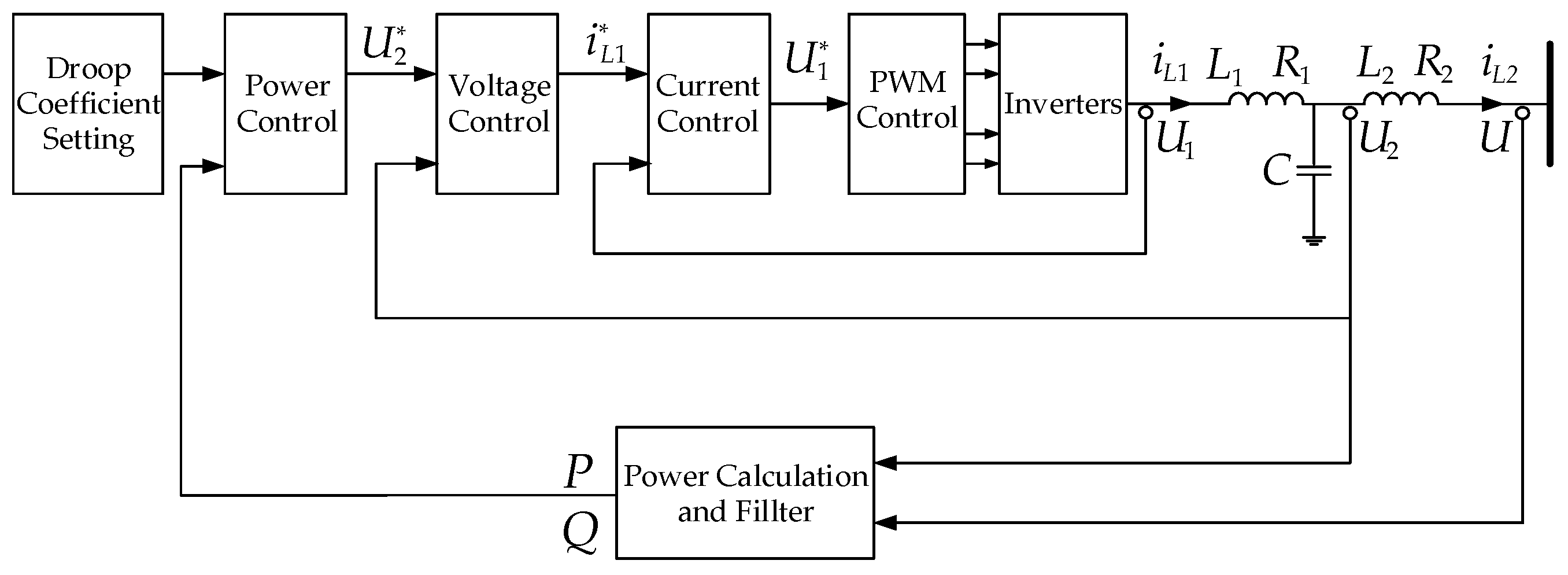
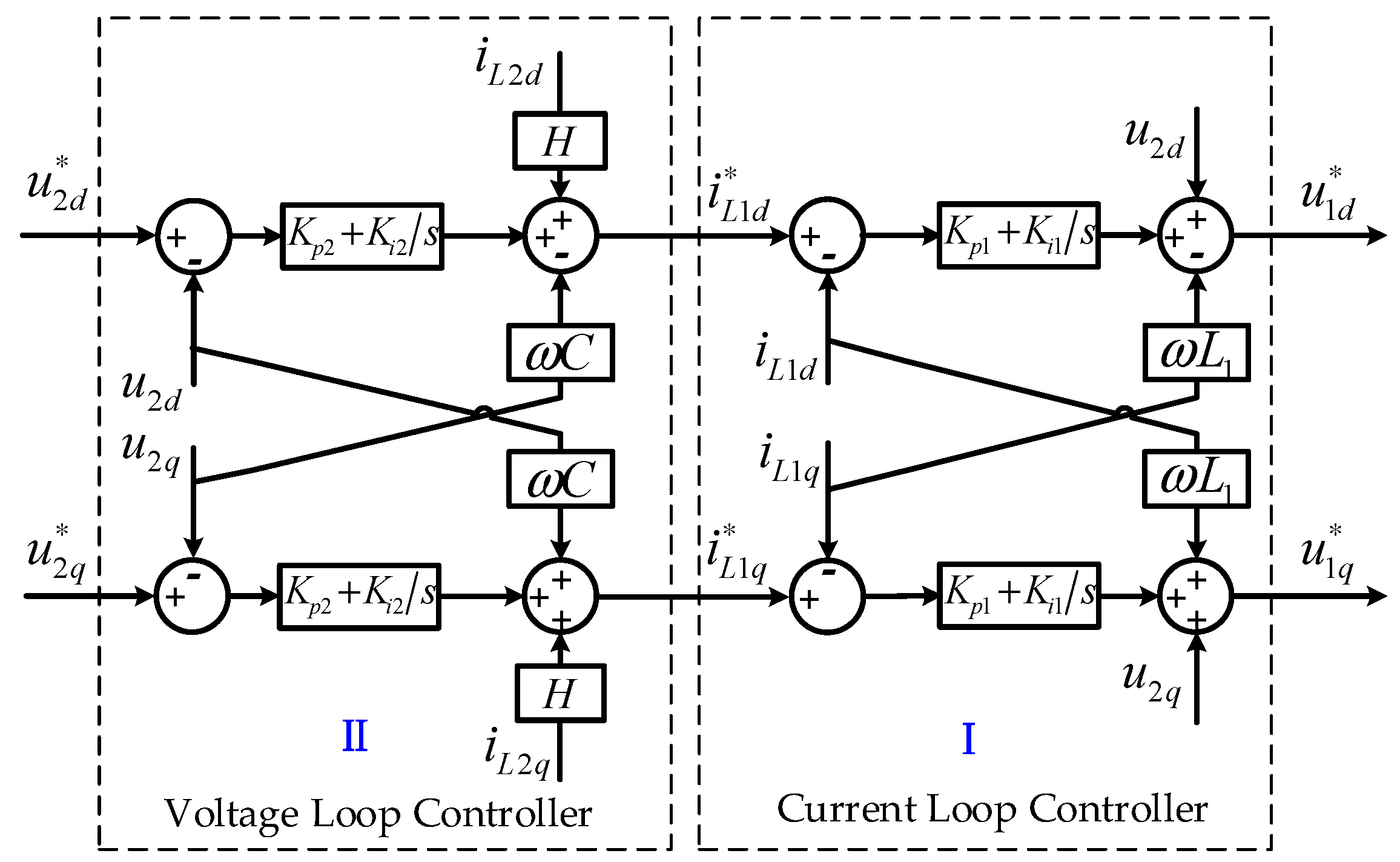
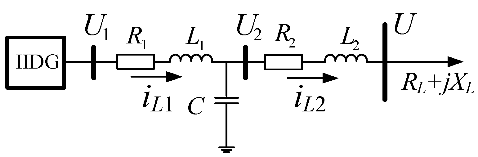
2.1. IIDG Full Model Based on Droop Control

(1) Power Droop Controller
The medium and high voltage microgrid generally has a voltage level of 10 kV and above with a large power supply capacity. The transmission line impedance is generally regarded as purely inductive, that is, ωL2 >> R2. In the low-voltage microgrid where the online transmission line impedance is resistive, realizing the conventional droop control of active power–frequency and reactive power–voltage through indirect transformation is feasible by using the improved droop control method based on virtual impedance and coordinate transformation. Thus, the output powers P and Q of an IIDG can be expressed as:
{ P = U 2 U sin δ ω L 2 Q = U 2 2 U 2 U cos δ ω L 2
where δ is the phase angle difference between the IIDG output voltage and the PCC voltage. Generally, the value of δ is very small, and the IIDG cannot directly control the PCC voltage. Thus, P is mainly determined by the output voltage phase angle, and Q is determined by the output voltage amplitude. The phase difference between two terminal voltages can be controlled by restricting the frequency of the output voltage, that is, controlling the active power P output by IIDG. Correspondingly, the reactive power Q output by IIDG can be controlled by managing the output voltage amplitude. Thus, the droop control of IIDG can be designed as follows:
{ ω = ω 0 m P U 2 = U 20 n Q
where ω0 and U20 are the reference values of the IIDG frequency and voltage, respectively; and m and n denote the active power and reactive power droop coefficients, respectively. Further, the instantaneous power of the IIDG can be calculated by its output voltage and current:
{ p = 3 2 ( u 2 d i L 2 d + u 2 q i L 2 q ) q = 3 2 ( u 2 d i L 2 q u 2 q i L 2 d ) .
The average power expression can be obtained through the low-pass filter:
{ P ( s ) = ω c s + ω c p Q ( s ) = ω c s + ω c q
where ωc is the cut-off frequency of the low-pass filter.
(2) Voltage and Current Dual-Loop Controller
Figure 2 shows that the voltage outer loop of the controller is regulated by PI (Proportional Integral). Meanwhile, the output current iL2 is introduced as the feedforward to suppress the influence of load fluctuation on the output voltage and improve the dynamic response performance of the system. The expression of the inner loop command current is as follows:
{ i L 1 d = H i L 2 d + K p 2 ( u 2 d u 2 d ) + K i 2 ( u 2 d u 2 d ) d t ω n C u 2 q i L 1 q = H i L 2 q + K p 2 ( u 2 q u 2 q ) + K i 2 ( u 2 q u 2 q ) d t + ω n C u 2 d .
The current inner loop adopts the inductor current feedback and PI regulation mode. The reference voltage of the current inner loop is:
{ u 1 d = u 2 d + K p 1 ( i L 1 d i L 1 d ) + K i 1 ( i L 1 d i L 1 d ) d t ω n L 1 i L 1 q u 1 q = u 2 q + K p 1 ( i L 1 q i L 1 q ) + K i 1 ( i L 1 q i L 1 q ) d t + ω n L 1 i L 1 d .
The state variables of the voltage outer and inner loops are defined to facilitate the problem analysis, as follows:
{ d φ d d t = u 2 d u 2 d d φ q d t = u 2 q u 2 q
{ d λ d d t = i L 1 d i L 1 d d λ q d t = i L 1 q i L 1 q .
(3) Filter and Line
The dynamic influence of the switching part can be neglected at high switching frequency. The switching tube can generate the required voltage in accordance with the instruction, that is, u1* = u1. Therefore, the d and q components of the filter inductance current iL1 are:
{ d i L 1 d d t = R 1 L 1 i L 1 d + ω i L 1 q + 1 L 1 ( u 1 d u 2 d ) d i L 1 q d t = ω i L 1 d R 1 L 1 i L 1 q + 1 L 1 ( u 1 q u 2 q ) .
The d and q axis components of its filter capacitance voltage U2 are:
{ d u 2 d d t = 1 C 1 ( i L 1 d i L 2 d ) + ω u 2 q d u 2 q d t = 1 C 1 ( i L 1 q i L 2 q ) ω u 2 d .
The d and q components of the output current iL2 on the line are shown below, where u is the voltage of PCC:
{ d i L 2 d d t = R 2 L 2 i L 2 d + ω i L 2 q + 1 L 2 ( u 2 d u d ) d i L 2 q d t = ω i L 2 d R 2 L 2 i L 2 q + 1 L 2 ( u 2 q u q ) .
The full system model of the IIDG is established by combining Equations (2)–(11), as shown in Equation (12):
{ x ˙ I I D G = A I I D G x I I D G + B I I D G u + F ( x I I D G ) x I I D G = [ δ P Q φ d q λ d q i L 1 d q u 2 d q i L 2 d q ] T u = [ u d u q ] T .
The expressions and parameters of the detailed model of the preceding equation are provided in Appendix A.

2.2. Multi-Time Scale Decomposition of IIDG System

The linear model of the IIDG full system can be obtained after linearization at the steady-state point, as shown in Equation (13):
{ Δ x ˙ I I D G = A S Δ x + B S Δ u Δ x I I D G = [ Δ δ Δ P Δ Q Δ φ d q Δ λ d q Δ i L 1 d q Δ u 2 d q Δ i L 2 d q ] T Δ u = [ Δ u d Δ u q ] T .
A stable operating point xs of the IIDG is taken. By solving the state matrix As of the linear model at the stable operating point, all characteristic roots of the IIDG model in the complex plane can be obtained, as shown in Table A1 and attached Figure A1. Appendix B provides the detailed elements of various matrixes in Equation (13).
According to Figure A1 and Table A1, the eigenvalues of the IIDG full model are distributed in several frequency bands with evident multi-time scale characteristics. The multi-time scale model of IIDG can be obtained through model simplification and perturbation factor extraction. According to the classification criterion of the multi-time scale [26], if the original system is stable with the characteristic spectrum, then the eigenvalues of the system state matrix As can be arranged from small to large. If the magnitude ratio of two adjacent eigenvalues, that is, the separation ratio, is less than 1, then this ratio can be used as the sign of time-scale division of the multi-time scale model.
The time scale is inversely proportional to the natural frequency or modulus of the characteristic root. A low natural frequency leads to small characteristic root modulus and long corresponding time scale. After referring to the calculation results of the eigenvalue modulus and separation ratio of the IIDG system in Appendix B, IIDG can be considered a typical three-time scale model. The voltage and current dual loop control should be integrated into one time scale. The characteristic time scale is 10−3 to 10−4 second level. The power outer loop control and the phase angle-frequency control should be classified into different time scales, namely, 10−2 and 10−1 second level, respectively.
The IIDG model comprises Equations (2) to (11) and is a 13-order differential equation set. Considering the preceding time-scale division principle, assuming:
{ x = δ y 1 = [ P Q ] T y 2 = [ φ d q λ d q i L 1 d q u 2 d q i L 2 d q ] T ε 1 = 1 / ω c , ε 2 = 1 / ω
where x is the state variable of IIDG phase angle, y1 denotes the state variable of the outer loop output power of IIDG, y2 represents the state variable of IIDG circuit equation and dual-loop control equation, and ε1 and ε2 refer to the corresponding perturbation parameters. Thus, the three-time scale system model of IIDG can be described as:
{ x ˙ = f ( x , y ) ε i y ˙ i = g ( x , y , u )
where i = 1, 2; f and g are the corresponding functional relations; and u represents the PCC voltage. Equation (15) is the expression form of Equation (12) after extracting the multi-time scale features.

2.3. Order Reduction Form of Neglecting Fast Dynamics for IIDG System

According to singular perturbation theory, when the singular perturbation parameter εi is sufficiently small and ε2 < ε1 << 1, the following two reduction forms can be obtained:
(1) Order Reduction Form 1 (ε2 = 0)
If the electromagnetic transient characteristics of the inductor current and capacitor voltage in the LCL filter circuit are neglected, then the corresponding voltage and current values are considered capable of following the instruction values at a rapid rate. Thus, the fast dynamics of the voltage and current dual-loop control and LCL filter circuit variables can be neglected, and the original model can be reduced to a third-order model with 12 algebraic constraint equations. The constraint equations are as follows:
K p 1 + R 1 L 1 [ i L 1 d i L 1 q ] + K p 1 H L 1 [ i L 2 d i L 2 q ] K p 1 K p 2 L 1 [ u 2 d u 2 q ] + K p 1 C L 1 [ u 2 q u 2 d ] + K p 1 K i 2 L 1 [ φ d φ q ] + K i 1 L 1 [ λ d λ q ] + K p 1 K i 2 L 1 [ u 2 d u 2 q ] = 0 R 2 ω L 2 [ i L 2 d i L 2 q ] + [ i L 2 q i L 2 d ] + 1 ω L 2 [ u 2 d u 2 q ] 1 ω L 2 [ u d u q ] = 0 1 ω C 1 [ i L 1 d i L 1 q ] 1 ω C 1 [ i L 2 d i L 2 q ] + [ u 2 q u 2 d ] = 0 [ u 2 d u 2 q ] = [ u 2 d u 2 q ] = [ ( U 20 n Q ) cos δ ( U 20 n Q ) sin δ ] 1 ω [ i L 1 d i L 1 q ] + H ω [ i L 2 d i L 2 q ] K p 2 ω [ u 2 d u 2 q ] + C [ u 2 q u 2 d ] +    K i 2 ω [ φ d φ q ] + K p 2 ω [ u 2 d u 2 q ] = 0 .
The power outer loop dynamic equation is as follows:
1 ω c d d t [ P Q ] = [ 1 0 0 1 ] [ P Q ] + 3 2 [ u 2 d u 2 q u 2 q u 2 d ] [ i L 2 d i L 2 q ] .
The phase angle equation is:
d δ d t = ω 0 m P .
(2) Order Reduction Form 2 (ε1 = 0, ε2 = 0)
If the measurement delay dynamics of the low-pass filter in the power outer loop control equation is neglected, that is, the fast dynamics of the active and reactive power variables in the power outer loop control are further neglected, then the original model can be reduced to a first-order model. Therefore, only the phase angle differential equation related to the frequency control and a set of algebraic equations are preserved. The new algebraic constraint equation is as follows:
[ 1 0 0 1 ] [ P Q ] + 3 2 [ u 2 d u 2 q u 2 q u 2 d ] [ i L 2 d i L 2 q ] = 0 .
Thus, the two order-reduction forms of the original system model are obtained. However, the stability consistency of the system after order reduction must be further verified.

3. Stability Consistency Proof of IIDG Model Order Reduction

The detailed mathematical model of the full IIDG system is a 13-order nonlinear model. The static and transient stability of the model after order reduction implementation are discussed. Static and transient stability are interrelated, but not equivalent; hence, providing the corresponding general proofs is necessary. The static and transient stability consistency proofs can verify the effectiveness of order reduction in theory. Besides, the stability consistency can be indirectly reflected by the dynamic response comparison between the detailed and reduction models.
Equation (20) is the general expression of a class of nonlinear multi-time scale mode corresponding to IIDG model. Considering the order reduction of neglecting fast dynamics on a rapid dynamic variable y ^ , the remaining slow state variables can be combined into the normal speed variable x ^ . εi can select any sufficiently small positive value ε:
{ d d t x ^ = f ( x ^ , y ^ ) ε i d d t y ^ i = g ( x ^ , y ^ , u ^ ) .

3.1. Consistency Proof of Static Stability before and after Order Reduction

The general form of the small signal model of the nonlinear multi-time scale system shown in Equation (20) at the equilibrium point can be expressed as [22]:
d d t [ Δ x ^ Δ y ^ ] = [ A 11 A 12 1 ε A 21 1 ε A 22 ] [ Δ x ^ Δ y ^ ] + [ B 1 1 ε B 2 ] Δ u ^ = A ( ε ) [ Δ x ^ Δ y ^ ] + B ( ε ) Δ u ^ .
The preceding equation is expressed in the complex frequency-domain form, as follows:
ε s I 2 Δ y ^ = A 21 Δ x ^ + A 22 Δ y ^ + B 2 Δ u ^ Δ y ^ = ( ε s I 2 A 22 ) 1 A 21 Δ x ^ + ( ε s I 2 A 22 ) 1 B 2 Δ u ^
s I 1 Δ x ^ = A 11 Δ x ^ + A 12 Δ y ^ + B 1 Δ u ^   = [ A 11 + A 12 ( ε s I 2 A 22 ) 1 A 21 ] Δ x ^ + [ B 1 + A 12 ( ε s I 2 A 22 ) 1 B 2 ] Δ u ^
where I1 and I2 are the same order unit matrix of Δ x ^ and Δ y ^ , respectively. Thus, the new state equation is:
s I 1 Δ x ^ = A n Δ x ^ + B n Δ u ^ .
By solving the characteristic root of Equation (24), the following equation can be obtained:
| s I 1 A n | = | s I 1 A 11 A 12 ( ε s I 2 A 22 ) 1 A 21 | = 0 .
According to the properties of the matrix Schur complement, the characteristic root of the system after order reduction satisfies Equation (25). When |sI2A22/ε| ≠ 0, ε ≠ 0, the corresponding characteristic roots of |sI1An| = 0 and |sIA| = 0 are the same:
| s I 1 A n | = | s I 1 A 11 A 12 ( ε s I 2 A 22 ) 1 A 21 | = | s I 1 A 11 A 12 A 21 ε s I 2 A 22 ε | | s I 2 A 22 ε |     | s I 2 A 22 ε | | s I 1 A n | = | s I 1 A 11 A 12 A 21 ε s I 2 A 22 |     = | s I 1 A 11 A 12 A 21 ε s I 2 A 22 ε | = | s I A | .
Owing to the small ε value, the following can be set when reducing the full model of the original system:
ε s I 2 Δ y ^ = 0 .
Thus, Equation (22) is further simplified as shown below after order reduction:
s I 1 Δ x ^ = [ A 11 A 12 A 22 1 A 21 ] Δ x ^ + [ B 1 A 12 A 22 1 B 2 ] Δ u ^ s I 1 Δ x ^ = A n Δ x ^ + B n Δ u ^ .
Subsequently, the characteristic equation of IIDG order reduction model satisfies the following equation (from the properties of the matrix Schur complement):
| A 22 | | s I 1 A n | = | A 22 | | s I 1 A 11 + A 12 A 22 1 A 21 | = | s I 1 A 11 A 12 A 21 A 22 | = 0 .
The following can be deduced by Equation (26):
| s I A | = | s I 1 A 11 A 12 A 21 ε s I 2 A 22 ε | .
When ε is close to 0:
| s I A | 1 ε | s I 1 A 11 A 12 A 21 A 22 | = | A 22 | ε | s I 1 A n | .
Therefore, the eigenvalues of the system order reduction model calculated by Equation (13) are all eigenvalues corresponding to the slow dynamic state variables in the full model of the original system, which is not related to ε.
By combining Equations (26) and (31), when ε is sufficiently small, the static stability of the original system is entirely determined by the stability of the order reduction system An and the boundary layer system A22 simultaneously. Hence, if and only if the order reduction and boundary layer systems are both stable, the original system can be stabilized; otherwise, the static stability may be inconsistent.

3.2. Consistency Proof of Transient Stability before and after Order Reduction

According to singular perturbation theory, when the singular perturbation parameter εi of a state variable is sufficiently small, the system of Equation (20) can be approximately decomposed into the following order reduction system:
{ d d t x ^ s = f ( x ^ s , y ^ s ) 0 = g ( x ^ s , y ^ s , u ^ )
and boundary layer system:
d d t x ^ s = f ( x ^ s , y ^ s ) ε i d d t y ^ f = g ( x ^ s ( t 0 ) , y ^ s ( t 0 ) + y ^ f , u ^ ) .
In Equation (31), x ^ s is a state variable with the initial value of x ^ s ( t 0 ) = x ^ 0 , and y ^ s denotes an algebraic variable with the initial value satisfying g ( x ^ s ( t 0 ) , y ^ s ( t 0 ) ) = 0 . In Equation (33), y ^ f represents a state variable. When εi is sufficiently small, the action time of the boundary layer system can be approximately viewed as short, and x ^ s will remain in its original value, thereby neglecting the rapid dynamic variable of the system.
Equations (20) and (32) correspond to the system before and after order reduction, respectively. These equations have completely consistent equilibrium points. If the dominant unstable equilibrium points (UEP) of the system before and after order reduction are both ( x ^ u , y ^ u ) , when εi selects any sufficiently small positive value ε, then the Jacobian matrix of the original system Equation (20) at the UEP is as follows:
J ( ε ) = [ f x f y g x ε g y ε ] = [ J 11 J 12 J 21 ε J 22 ε ]
where J 11 = f x = ( f / x ^ ) | ( x ^ u , y ^ u ) ; J 12 = f y = ( f / y ^ ) | ( x ^ u , y ^ u ) ; J 21 = g x = ( g / x ^ ) | ( x ^ u , y ^ u ) ; and J 22 = g y = ( g / y ^ ) | ( x ^ u , y ^ u ) .
If the left eigenvector of the unstable eigenvalue J ( ε ) of μ ( ε ) is expressed as η ( ε ) = [ η 1 T ( ε ) η 2 T ( ε ) ] T , in which η 1 ( ε ) is (nn0) × 1 column vector and η 2 ( ε ) is n0 × 1 column vector, then:
J T ( ε ) η ( ε ) = [ J 11 T J 21 T ε J 12 T J 22 T ε ] [ η 1 ( ε ) η 2 ( ε ) ] = μ ( ε ) [ η 1 ( ε ) η 2 ( ε ) ] .
If J22 is reversible, then the following can be obtained by Equation (35):
lim ε 0   η 2 ( ε ) ( ε J 22 T J 12 T η 1 ( ε ) ) = 0
( J 11 T J 21 T J 22 T J 12 T ) lim ε 0   η 1 ( ε ) lim ε 0   μ ( ε ) lim ε 0   η 1 ( ε ) .
Similarly, the Jacobian matrix of the order reduction system Equation (32) at the UEP ( x ^ u , y ^ u ) can be further deduced to the following:
J = J 11 J 12 J 22 1 J 21 .
Assuming μ′, the unstable eigenvalues of J′, which has the left eigenvector of η 1 , then:
J T η 1 = ( J 11 T J 21 T J 22 T J 12 T ) η 1 = μ η 1 .
If J′ and J(ε) have the same unstable eigenvalue when ε is sufficiently small, that is., μ = lim ε 0   μ ( ε ) , then η 1 C 1 lim ε 0   η 1 ( ε ) can be obtained after comparing Equations (37) and (39). C1 is a constant.
The stability region boundary function of the original system (20) is constructed in this study according to the quadratic approximation method of the stability region boundary of the nonlinear system [27]. The function can be expressed as follows:
h Q ( x ^ , y ^ , ε ) = η T ( ε ) [ x ^ x ^ u y ^ y ^ u ] + 1 2 [ x ^ x ^ u y ^ y ^ u ] T Ψ ( ε ) [ x ^ x ^ u y ^ y ^ u ] .
Among the preceding equations, the coefficient matrix of the quadratic term Ψ ( ε ) satisfies the following Lyapunov matrix equation:
C ( ε ) Ψ ( ε ) + Ψ ( ε ) C T ( ε ) = H
where Ψ ( ε ) = [ Ψ 11 ( ε ) Ψ 12 ( ε ) Ψ 12 T ( ε ) Ψ 22 ( ε ) ] , in which Ψ 11 ( ε ) is (nn0)×(nn0) matrix; Ψ 12 ( ε ) denotes (nn0) × n0 matrix; Ψ 22 ( ε ) refers to n0 × n0 matrix; C ( ε ) = ( μ ( ε ) I n / 2 J T ( ε ) ) ; In represents n order unit matrix; and H, which is expressed below, denotes the Hessian matrix of the function at the equilibrium point ( x ^ u , y ^ u ) :
H = i = 1 n n 0 ( η 1 ( ε ) ) i H s ( f i ) + 1 ε j = 1 n 0 ( η 2 ( ε ) ) j H s ( g j )
where ( η 1 ( ε ) ) i is the ith element of η 1 ( ε ) ; ( η 2 ( ε ) ) j denotes the jth element of η 2 ( ε ) ; and H s ( f i ) H s ( g j ) , which are expressed below, represent the Hessian matrixes of fi and gj at the UEP, respectively ( x ^ u , y ^ u ) ; i = 1, 2, …, nn0, j = 1, 2…, n0:
H s ( f i ) = [ H x x f i H x y f i ( H x y f i ) T H y y f i ] = [ 2 f i x ^ 2 2 f i x ^ y ^ ( 2 f i x ^ y ^ ) T 2 f i y ^ 2 ]
H s ( g j ) = [ H x x g j H x y g j ( H x y g j ) T H y y g j ] = 1 ε [ 2 g j x ^ 2 2 g j x ^ y ^ ( 2 g j x ^ y ^ ) T 2 g j y ^ 2 ] .
Based on the assumption that ε is sufficiently small and the eigenvalue of J22 has strictly negative realness, Equation (40) is expanded and further expressed as follows:
Ψ 11 ( ε ) ( μ ( ε ) I n n 0 2 J ) + ( μ ( ε ) I n n 0 2 J T ) Ψ 11 ( ε ) i = 1 n n 0 ( η 1 ( ε ) ) i H i f j = 1 n 0 ( J 22 T J 12 T η 1 ( ε ) ) j H j g .
The specific deduction proof is shown in Appendix C. In the previous equation:
H i f = H x x f i H x y f i J 22 1 J 21 J 21 T J 22 T ( H x y f i ) T + J 21 T J 22 T H x x f i J 22 1 J 21
H j g = H x x g j H x y g j J 22 1 J 21 J 21 T J 22 T ( H x y g j ) T + J 21 T J 22 T H y y g j J 22 1 J 21 .
Similarly, the stability region boundary function of the order reduction system Equation (32) is:
h Q ( x ^ ) = η T ( x ^ x ^ u ) + 1 2 ( x ^ x ^ u ) T Ψ ( x ^ x ^ u )
where Ψ is the (nn0) × (nn0) coefficient matrix of the quadratic coefficient. The Lyapunov matrix equation is also satisfied, which can be expressed as follows:
Ψ ( μ ( ε ) I n n 0 2 J ) + ( μ ( ε ) I n n 0 2 J T ) Ψ i = 1 n n 0 ( η 1 ) i H i f j = 1 n 0 ( J 22 T J 12 T η 1 ) j H j g .
The following can be obtained after comparing the preceding equation and Equation (44):
Ψ C 2 lim ε 0   Ψ 11 ( ε ) .
Therefore, the stability region boundary functions of the original and order reduction systems have the following relations:
h Q ( x ^ ) C 2 lim ε 0   h Q ( x ^ , y ^ , ε ) .
According to the definition of the transient stability index in stability region boundary theory of the nonlinear system [28], the transient stability index of the original system is defined as follows:
I Q ( x ^ 0 , y ^ 0 , ε ) = h Q ( x ^ 0 , y ^ 0 , ε ) h Q ( x ^ s , y ^ s , ε ) .
The transient stability index of the order reduction system is defined as:
I Q ( x ^ 0 ) = h Q ( x ^ 0 ) h Q ( x ^ s ) .
( x ^ s , y ^ s ) is the stable equilibrium point (SEP) of the original and order reduction systems. The transient stability indexes before and after order reduction should satisfy the following relations:
I Q ( x ^ 0 ) lim ε 0   I Q ( x ^ 0 , y ^ 0 , ε ) .
The sufficient condition for Equation (52) is that the eigenvalue of J22 has the strictly negative realness. Moreover, the transient stability of the original system and the order reduction system is consistent, and the transient stability indexes are approximately equal. According to the introduction of stability region boundary theory in [28], the transient stability index reflects whether the operating point of the system is within the stability region boundary. When the system is stable, the transient stability index is positive; when the system is unstable, the transient stability index is negative; when the system is zero, the system is in the critical stable state. Table 1 shows the transient stability law.

3.3. Consistency Evaluation of Dynamic Response before and after Order Reduction

In order to evaluate the dynamic response consistency of the system state variables before and after the order reduction, the Prony transformation is used to extract the three crucial characteristics of dynamic response: frequency, damping and amplitude [29]. The Prony transformation describes the time-series sampling data of dynamic response by a set of linear combinations of exponential function. Through the appropriate expansion [30], the frequency, damping coefficient, amplitude and initial phase angle of a given sampling data can be estimated. Three consistency indexes of frequency, damping and amplitude are applied to represent the error of dynamic response. By the Prony transformation on the dynamic response of the original detailed system, the frequency and energy can be written as:
{ F d = ( f d 1 ,   f d 2 ,   , f d n ) E d = ( λ d 1 ,   λ d 2 ,   , λ d n )
where fdi and λdi (i = 1, 2…n) are the frequency and energy of the ith element for the dynamic response of detailed system. The frequency and energy of order reduction models can also be obtained by same transformation as:
{ F s = ( f s 1 ,   f s 2 ,   f s n ) E s = ( λ s 1 ,   λ s 2 ,   , λ s n )
where fsi and λsi (i = 1, 2…n) are the frequency and energy of the ith element of the reduction model.
(1) Consistency index of frequency
The frequency consistency index of the reduction model can be obtained by comparing the frequency vectors of Fd and Fs. The non-periodic signals are useless for analyzing frequency information, so the non-periodic signals are removed in the calculation of frequency consistency. The energy signal of each element is chosen as the weight in calculating the consistency of the frequency. The frequency consistency is defined as:
w i = λ d i i = 1 n λ d i
σ i = 1 | f d i f s i max ( f d i , f s i ) |
φ f = i = 1 n w i σ i
where σi and wi are the frequency consistency and weight of ith element; ϕf is the frequency consistency index of dynamic response for the order reduction model.
(2) Consistency index of damping
Same with the frequency consistency, the damping consistency index can be obtained as:
η i = { 1 | ξ d i ξ s i max ( ξ d i , ξ s i ) | , ξ d i ξ s i > 0 0 , ξ d i ξ s i < 0
φ ξ = i = 1 n w i η i ,
where ηi is the damping consistency of the ith element; ξdi and ξsi are the damping of the ith element for the detailed model and the reduction model calculated by the Prony transformation [30]; ϕξ is the damping consistency index of the dynamic response for the order reduction model. It is noted that the ηi could be zero when ξdi and ξsi having different sign, which means the dynamic response of these two models have the opposite stability trend, and the damping characteristic of these two elements are independent.
(3) Consistency index of amplitude
Similarly, the amplitude consistency index can be given as:
ε i = 1 | A d i A s i max ( A d i , A s i ) |
φ A = i = 1 n w i ε i ,
where εi is the amplitude consistency of the ith element; Adi and Asi are the amplitudes of ith element for the detailed model and the reduction model respectively; ϕA is the amplitude consistency index of dynamic response for order reduction models. These three consistency indexes are between 0 and 1. The more closely they approach 1, the more the higher similarity they have.

4. Simulation Studies

The effectiveness of IIDG order reduction is verified by the static and transient stability consistency proofs in Section 3. In Section 4, the simulation results are used as well to verify the effectiveness of order reduction through a stand-alone case and a practical microgrid cases. Verifications mainly include the comparisons of eigenvalue, transient stability index and time-domain waveform between original model and different order-reduction models.

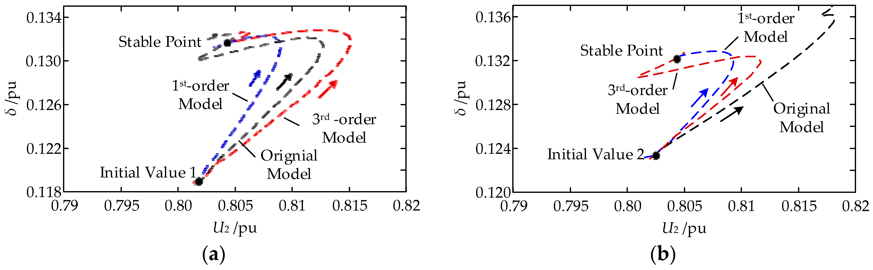
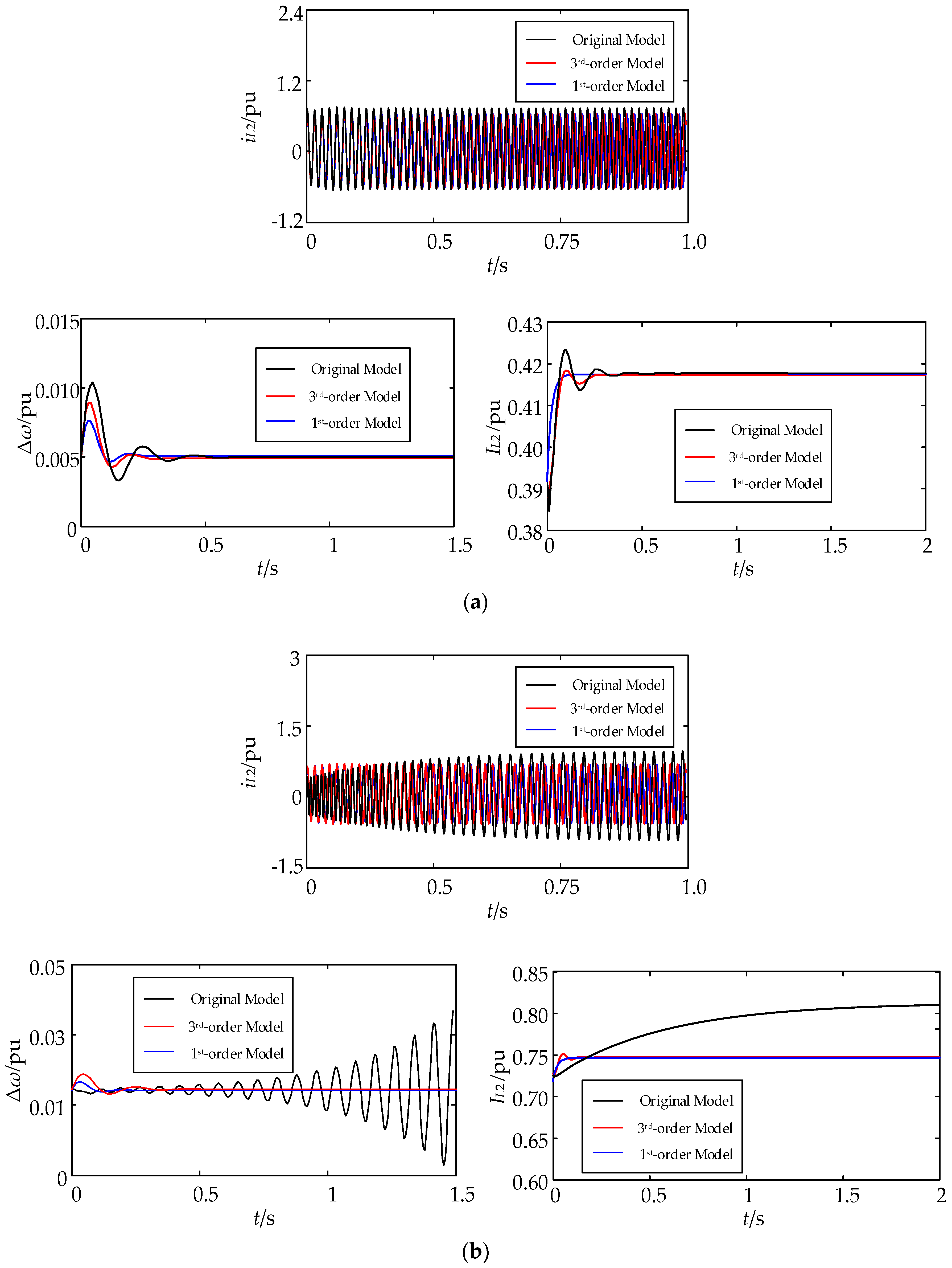
4.1. Stand-Alone System (System 1)

The example system in Figure 3 is selected to verify the effectiveness of the preceding order reduction system presented. An IIDG is connected to the PCC via the LCL circuit, in which the IIDG full model has 13 orders, including three orders of outer loop power droop controller, four orders of voltage and current dual-loop controller, and six orders of filter and line. The detailed simulation parameters of System 1 are consistent with the IIDG system provided in Appendix A.
Table 2 shows the initial values and operating equilibrium points of various state variables of IIDG. Under the operating condition of the SEP, the small signal stability of System 1 is analyzed. The eigenvalues of the system before and after order reduction can be obtained by solving the state matrix, as shown in Table 3.
Order Reduction Form 1 is a third-order model that reserves the power outer loop control equation and the phase angle equation, whereas Order Reduction Form 2 is a first-order model that reserves only the phase angle equation. According to the calculation results in Table 3, the order reduction precision of the third-order model is higher than that of the first-order model. However, if the rapid dynamic reduction form is neglected, then the static stability consistency of both models before and after order reduction can be guaranteed.
Table 4 shows that the transient stability index of the original system IQ(x0, y0, ε) is 0.7989 under the effect of Initial Value 1, which indicates the stability of the original system. At this point, the transient stability indexes of the third- and first-order systems are 0.8240 and 0.6241, respectively. They are of the same sign as the transient stability index of the original system, and the order reduction systems are in the stable state. In addition, J22 is found to guarantee the strictly negative realness of the eigenvalues under two order reduction forms through calculation, which means that the transient stability of the system before and after order reduction is consistent.
Under the effect of Initial Value 2, the transient stability index of the original system IQ(x0, y0, ε) is −0.0033. During this time, the transient stability indexes of the third- and first-order systems are 0.0054 and 0.2080, respectively. The transient stability indexes before and after order reduction are of different signs. The original system is unstable, and the order reduction systems are in the stable system. In addition, J22 cannot guarantee the strictly negative realness of the eigenvalues through calculation. In other words, under the precise original system instability, the transient stability of the system before and after order reduction is inconsistent, which corresponds to the third analysis case in Table 1. The calculation time of different models are also shown in Table 4. Due to the reduced complexity of the model, 1st order model takes less calculation time than 3rd order model.
The δ-U2 solution curves of the original and order reduction systems are obtained under the effect of two initial values through time-domain simulation, as shown in Figure 4. Under the effect of Initial Value 1, the solution curves of the original system model and the order reduction system model in Figure 4a can converge to a SEP. However, under the effect of Initial Value 2, the solution curve of the original system in Figure 4b cannot converge to the SEP. The time-domain simulation of the curve in Figure 4 indirectly verifies the transient stability index analysis results.
Figure 5a,b are the time-domain simulation results of the system under the small disturbance, where iL2, IL2, and Δω are the instantaneous current, frequency deviation, and RMS (Root-Mean-Square) current of IIDG output respectively. The small disturbance form is that PCC voltage U steps from 1.0 to 1.05. The dynamic response results in Figure 5a further verify the stability analysis results of the preceding table. At the SEP, the stability of the system remains unchanged before and after order reduction. Figure 5b corresponds to the instability of the original system. During this time, the order reduction system remains stable. Hence, the stability consistency of the system cannot be guaranteed under the condition of original system instability. Table 5 shows the calculation results of three consistency indexes of dynamic response for the IIDG output current in Figure 5a. When operating at stable point, high values of these three consistency indexes are presented which clearly means that the difference of dynamic responses between the order reduction models and original model are relatively small.

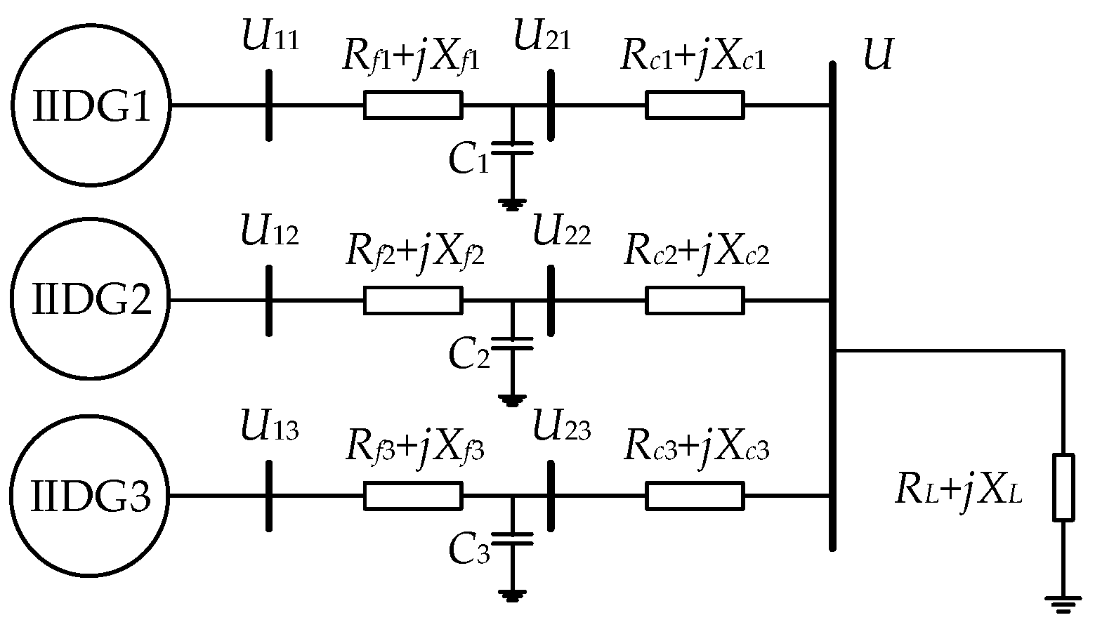
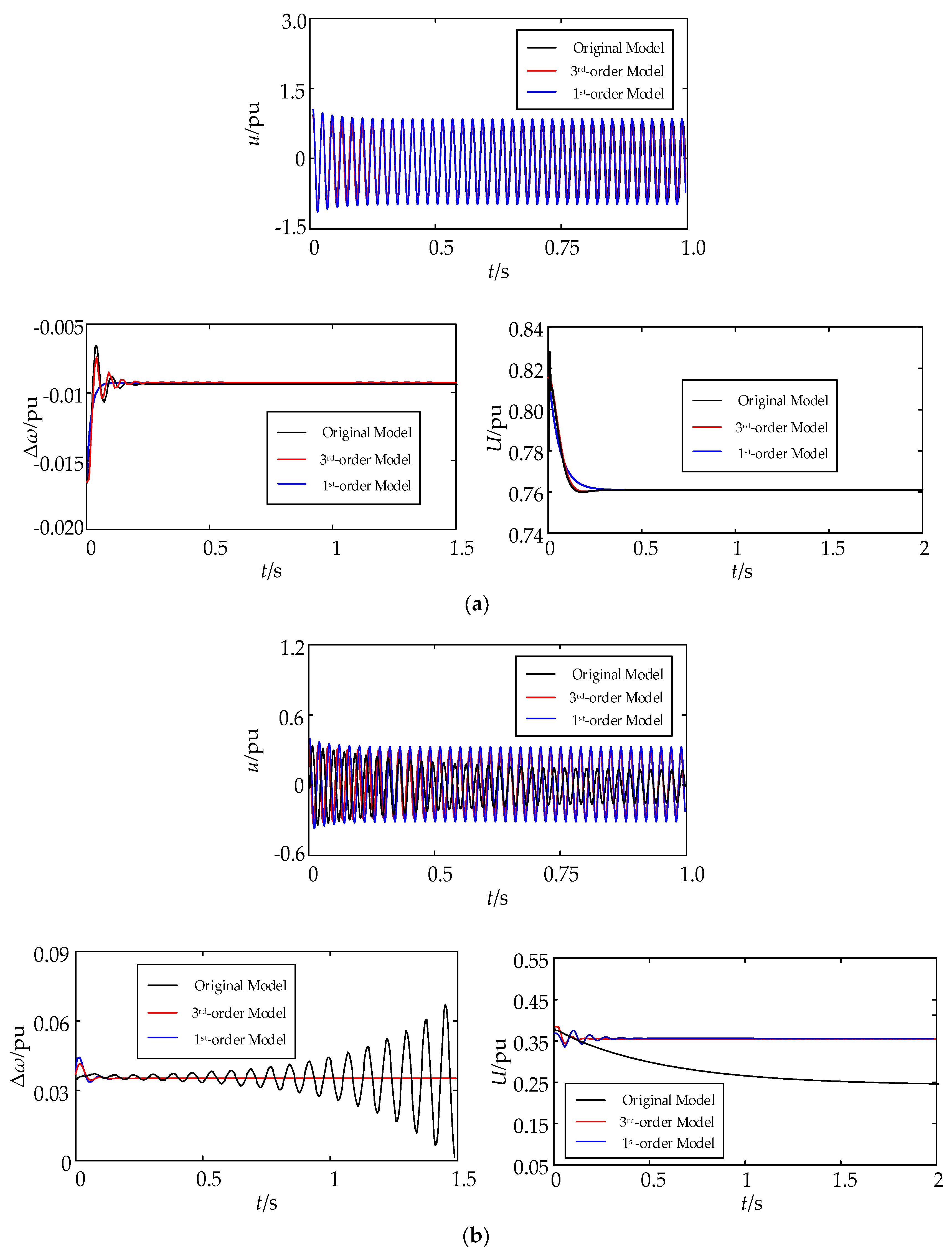
4.2. Three-IIDG Microgrid Pilot Project System (System 2)

The distributed photovoltaic power generation and microgrid operation control pilot project at the Henan College of Finance and Taxation under practical operation is selected as a simulation example. In the pilot project, the system capacity is 380 kW PV and two × 100 kW/kWh energy storage. The network structure can be equivalent to the microgrid with three IIDGs connected in parallel (two energy storage power sources and a PV power source), as shown in Figure 6. Appendix D presents the detailed parameters of System 2. Table 6 shows the initial values and operating equilibrium points of the state variables.
The eigenvalues of the system before and after order reduction can be obtained through the small signal stability analysis of the microgrid system under the SEP condition. Each IIDG uses two order reduction models deducted in the paper, namely, the third- and first-order models. The complete 39-order microgrid model selects only the dominant eigenvalues to analyze the problem, and all order reduction models are processed by neglecting fast dynamics to only analyze the eigenvalues of the slow subsystem, as shown in Table 7.
From the analysis results in Table 7, the static stability consistency of the three-IIDG microgrid system before and after order reduction can be guaranteed under the premise of neglecting the variable dynamics of the system. When IIDG uses the third-order model for order reduction, the eigenvalue of the slow subsystem and the static stability are relatively close to the dominant eigenvalue of the original system. The eigenvalue of the system with the first-order model is significantly different from that of the original system but can still guarantee the static stability of the system.
Table 8 further analyzes the eigenvalues of System 2 at the UEP before and after order reduction and finds that the original and order reduction systems of IIDG using the third-order model are unstable. However, the IIDG using the first-order model for order reduction remains stable. In other words, considering system instability, the order reduction of IIDG by the third-order model is suitable for the simulation results of the original system. Therefore, based on the analysis results in Table 6, the static stability of IIDG using the third-order reduction model is better than that of IIDG using the first-order model.
Table 9 further analyzes the transient stability of System 2 at Initial Values 3 and 4 before and after the order reduction. Under the effect of Initial Value 3, the transient stability indexes of the original and order reduction systems are consistent. Under the effect of Initial Value 4, the transient stability indexes of the original and third-order systems are negative and those of the first-order system are positive. For the first-order system, under the premise that the original system is unstable, the transient stability consistency cannot be guaranteed. Thus, the transient stability of the system using the third-order reduction model is better than that of the system using the first-order reduction model. The calculation time comparison of different cases in Table 9 shows that the time saving is still impressive for the reduction models of IIDG. The finding implies that the larger the test system is, the more significant the improved computational efficiency will be. Especially for the 1st model, the calculation time is nearly unchanged comparing with the standalone case. However, comprehensively considering transient stability and calculation time, the 3rd order model has a better performance than adopting 1st order model.
Figure 7 further presents the projections of the stability region boundary of System 2 on the δ1δ2 phase plane before and after order reduction, in which A and B are the projections of Initial Values 3 and 4, respectively. The stability region boundary curve shows that the system stability region is closer to that of the original system compared with that of the first-order model after IIDG adopts the third-order model for order reduction. As Initial Value 3 (Point A) is within three stability region boundaries, the transient stability consistency of this value before and after order reduction must be guaranteed. If Initial Value 4 (Point B) is outside the stability region boundaries of the original and third-order systems and located in that of the first-order system, then the transient stability consistency of IIDG before and after order reduction can be guaranteed by taking the third-order model. However, transient stability consistency cannot be guaranteed if the first-order model is used. This result is consistent with the transient stability index analysis results in Table 8.
Figure 8a,b are the time-domain simulation results of the microgrid system under the small disturbance happened in load, where u, U, and Δω are the instantaneous voltage, RMS voltage, and frequency deviation at PCC respectively. The small disturbance form is the load demand steps from 1.0 to 1.1. When operating at SEP, the stability of the system remains unchanged with IIDG adopting two different order reduction models (1st and 3rd). However, at UEP in Figure 6b, the stability consistency of the system cannot be guaranteed under the condition of original system instability. Table 10 show the calculation results of three consistency indexes for the microgrid PCC voltage dynamic response in Figure 8a. For operating at stable point, high values demonstrate the good match between the order reduction system and original system.

5. Conclusions

This study establishes the full detailed model for IIDG based on the droop control in microgrid, extracts the multi-time scale singular perturbation parameters of the model according to singular perturbation theory, implements the order reduction processing of neglecting fast dynamics, and proposes the simplified first and third-order reduction models. Then, this study verifies the static and transient stability consistency of the system before and after order reduction by theoretical derivation and introduction of the quadratic approximation method of the stability region boundary. The results show that the static and transient stability consistency of the IIDG system before and after order reduction can be guaranteed when the original system operating at stable state. Through the eigenvalue comparisons, the transient stability index comparisons and time-domain waveform results of the stand-alone system and the microgrid system, the effectiveness of the time-scale division and order reduction processing of the IIDG full model are finally proved.

Acknowledgments

This work was supported by the Chongqing Research Program of Basic Research and Frontier Technology (cstc2015jcyjBX0033), National Natural Science Foundation of China (51577018) and Fundamental Research Funds for the Central Universities (No. 106112016CDJXY150001).

Author Contributions

Xiaoxiao Meng and Qianggang Wang contributed to paper writing and the whole revision process. Niancheng Zhou and Xiaoxiao Meng built the simulation model and analyzed the data. Shuyan Xiao and Yuan Chi helped organize the article. All the authors have read and approved the final manuscript.

Conflicts of Interest

The authors declare no conflict of interest.

Appendix A

Appendix A.1. IIDG Parameters

Pn = 120 kVA, Un = 208 V, fn = 50 Hz, L1 = 1.5 mH, R1 = 0.15 Ω, C = 45 μF, L2 = 0.53 mH, R2 = 0.05 Ω, m = 1 × 10⁻⁴ rad/s/W, n = 1 × 10⁻³ V/Var, ωc = 30 rad/s, ωn = 101 πrad/s, Kp1 = 10, Ki1 = 15,000, Kp2 = 0.048, Ki2 = 400, H = 0.65, P = 50 kW, Q = 5 kVar.

Appendix A.2. IIDG Detailed Model

A I I D G = [ A P Q 0 0 A C V ] ;   B = [ 0 B C V ] ;   F ( x ) = [ F 1 F 2 F 3 ]
A P Q = [ 0 m 0 0 ω c 0 0 0 ω c ]
A C V = [ 0 0 0 0 0 0 1 0 0 0 0 0 0 0 0 0 0 1 0 0 K i 2 0 0 0 1 0 K p 2 ω n C H 0 0 K i 2 0 0 0 1 ω n C K p 2 0 H K p 1 K i 2 L 1 0 K i 1 L 1 0 K p 1 + R 1 L 1 ω ω n K p 1 K p 2 L 1 K p 1 ω n C L 1 K p 1 H L 1 0 0 K p 1 K i 2 L 1 0 K i 1 L 1 ω n ω K p 1 + R 1 L 1 K p 1 ω n C L 1 K p 1 K p 2 L 1 0 K p 1 H L 1 0 0 0 0 1 C 0 0 ω 1 C 0 0 0 0 0 0 1 C ω 0 0 1 C 0 0 0 0 0 0 1 L 2 0 R 2 L 2 ω 0 0 0 0 0 0 0 1 L 2 ω R 2 L 2 ]
B I I D G = [ 0 0 1 L 2 0 0 0 0 1 L 2 ] 2 × 13 T
F 1 = [ ω n 3 2 ω c ( u 2 d i L 2 d + u 2 q i L 2 q ) 3 2 ω c ( u 2 d i L 2 q u 2 q i L 2 d ) ] ;   F 2 = [ ( U 20 n Q ) cos δ ( U 20 n Q ) sin δ K p 2 ( U 20 n Q ) cos δ K p 2 ( U 20 n Q ) sin δ ] ;   F 3 = [ K p 1 K p 2 L 1 ( U 20 n Q ) cos δ K p 1 K p 2 L 1 ( U 20 n Q ) sin δ 0 0 0 0 ] .

Appendix B

Figure A1 and Table A1 show that the eigenvalues of the IIDG complete model are distributed in multiple frequency bands, with significant multi-time scale characteristics. The IIDG multi-time scale model can be obtained by using strict model simplification and extracting perturbation factors. According to the principle of the multi-time scale division, if the system remains stable and has a characteristic spectrum, then the eigenvalues of system state matrix As can be arranged from small to large based on their absolute values, which can be shown as follows:
0 < 3 < 29.68 < 300 < 0.19 × 10⁴ < 0.29 × 10⁴ < 0.30 × 10⁴ < 1.23 × 10⁴
Table A1. Eigenvalues of IIDG detailed model.
EigenvaluesValues
λ1,2−1.2277 × 10⁴ ± 0.0332 × 10⁴i
λ3,4−0.0689 × 10⁴ ± 0.2954 × 10⁴i
λ5,6−0.085 × 10⁴ ± 0.281 × 10⁴i
λ7,8−0.189 × 10⁴ ± 0.007 × 10⁴i
λ9,10−0.011 × 10⁴ ± 0.030 × 10⁴i
λ11,12−16 ± 25i
λ13−3
Figure A1. Eigenvalue diagram of IIDG detailed model, where the red circle indicates the dominant low-frequency eigenvalues.
Energies 11 00254 g0a1
Among the preceding values, the separation ratios can be presented as μ1 = 29.68/300 = 0.099 << 1, μ2 = 3/29.68 = 0.101 << 1, which can be viewed as the marks of the multi-time scale division. Therefore, the model of IIDG is a standard three-time scale model.

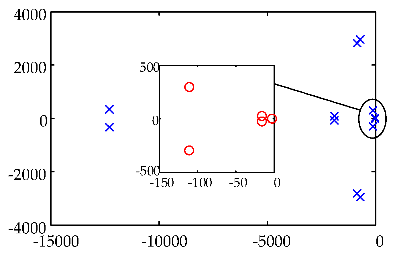
State Matrix of the IIDG Complete Model

A S = [ 0 m 0 0 0 0 0 0 0 0 0 0 0 0 ω c 0 0 0 0 0 0 0 1.5 ω c I L 2 d 1.5 ω c I L 2 q 1.5 ω c U 2 d 1.5 ω c U 2 q 0 0 ω c 0 0 0 0 0 0 1.5 ω c I L 2 q 1.5 ω c I L 2 d 1.5 ω c U 2 q 1.5 ω c U 2 d ( U n n Q 0 ) sin δ 0 0 n cos δ 0 0 0 0 0 0 0 1 0 0 0 ( U n n Q 0 ) cos δ 0 0 n sin δ 0 0 0 0 0 0 0 0 1 0 0 K p 2 ( U n n Q 0 ) sin δ 0 0 n K p 2 cos δ 0 K i 2 0 0 0 1 0 K p 2 ω n C H 0 K p 2 ( U n n Q 0 ) cos δ 0 0 n K p 2 sin δ 0 0 K i 2 0 0 0 1 ω n C K p 2 0 H K p 1 K p 2 L 1 ( U n n Q 0 ) cos δ 0 m I L 1 q n K p 1 K p 2 L 1 cos δ 0 K p 1 K i 2 L 1 0 K i 1 L 1 0 K p 1 + R 1 L 1 ω ω n K p 1 K p 2 L 1 K p 1 ω n C L 1 K p 1 H L 1 0 K p 1 K p 2 L 1 ( U n n Q 0 ) cos δ 0 m I L 1 d n K p 1 K p 2 L 1 sin δ 0 0 K p 1 K i 2 L 1 0 K i 1 L 1 ω n ω K p 1 + R 1 L 1 K p 1 ω n C L 1 K p 1 K p 2 L 1 0 K p 1 H L 1 0 m U 2 q 0 0 0 0 0 1 C 0 0 ω 1 C 0 0 m U 2 d 0 0 0 0 0 0 1 C ω 0 0 1 C 0 m I L 2 q 0 0 0 0 0 0 0 1 L 2 0 R 2 L 2 ω 0 m I L 2 d 0 0 0 0 0 0 0 0 1 L 2 ω R 2 L 2 ]
B S = [ 0 0 0 0 0 0 0 0 0 0 0 1 L 2 0 0 0 0 0 0 0 0 0 0 0 0 0 1 L 2 ] T .

Appendix C

Ψ 11 ( ε ) ( μ ( ε ) I n n 0 2 J 11 ) + ( μ ( ε ) I n n 0 2 J 11 T ) Ψ 11 ( ε ) Ψ 12 ( ε ) J 21 ε J 21 T Ψ 12 T ( ε ) ε = S x x
Ψ 12 ( ε ) ( μ ( ε ) I n 0 2 J 22 ε ) + ( μ ( ε ) I n n 0 2 J 11 T ) Ψ 12 ( ε ) Ψ 11 ( ε ) J 12 J 21 T Ψ 22 ( ε ) ε = S x y
Ψ 12 T ( ε ) ( μ ( ε ) I n n 0 2 J 22 ε ) + ( μ ( ε ) I n 0 2 J 22 T ε ) Ψ 12 T ( ε ) J 12 T Ψ 11 ( ε ) Ψ 22 ( ε ) J 21 ε = S x y T
Ψ 22 ( ε ) ( μ ( ε ) I n 0 2 J 22 ε ) + ( μ ( ε ) I n 0 2 J 22 T ε ) Ψ 22 ( ε ) Ψ 12 T ( ε ) J 12 J 12 T Ψ 12 ( ε ) = S y y .
In the preceding equations:
S x x = i = 1 n n 0 ( η 1 ( ε ) ) i H x x f i + 1 ε j = 1 n 0 ( η 2 ( ε ) ) j H x x g j ;   S x y = i = 1 n n 0 ( η 1 ( ε ) ) i H x y f i + 1 ε j = 1 n 0 ( η 2 ( ε ) ) j H x y g j ;
S y y = i = 1 n n 0 ( η 1 ( ε ) ) i H y y f i + 1 ε j = 1 n 0 ( η 2 ( ε ) ) j H y y g j .
Matrix T1 is defined as J 22 T I n 0 + I n 0 J 22 T , where can be viewed as the tensor product mapping mark of semi-tensor product algorithm. If T1 is invertible, then Equation (A11) can be derived as:
Ψ 22 ( ε ) = ε V c 1 ( I n 0 2 ε μ ( ε ) T 1 1 ) T 1 1 V c ( S y y + Ψ 12 T ( ε ) J 12 + J 12 T Ψ 12 ( ε ) )
where Vc is the column vector accumulation mapping in the semi-tensor algorithm. Ψ 22 ( ε ) is infinitesimal of the same order with ε, which means lim ε 0   Ψ 22 ( ε ) = 0 . Assuming that T 2 = J 22 T I n n 0 , T 3 = μ ( ε ) I n 0 × ( n n 0 ) I n 0 J 11 T , and T2 is reversible, then Equation (A13) can be obtained from Equation (A9).
Ψ 12 ( ε ) = ε V c 1 ( I n 0 × ( n n 0 ) ε T 3 T 2 1 ) T 2 1 V c ( S x y + Ψ 11 ( ε ) J 12 + J 21 T Ψ 22 ( ε ) ε ) .
Plugging Equation (A9) into (A13) to find that Ψ 12 ( ε ) is also infinitesimal of the same order with ε, that is, lim ε 0   Ψ 12 ( ε ) = 0 .
Combining Equations (A8) to (A13), (A14) can be derived as follows:
Ψ 11 ( ε ) ( μ ( ε ) I n n 0 2 J ) + ( μ ( ε ) I n n 0 2 J T ) Ψ 11 ( ε ) = i = 1 n n 0 ( η 1 ( ε ) ) i H i f + 1 ε j = 1 n 0 ( η 2 ( ε ) ) j H j g .
Considering the relationship with Equation (35), (A14) can be further represented as:
Ψ 11 ( ε ) ( μ ( ε ) I n n 0 2 J ) + ( μ ( ε ) I n n 0 2 J T ) Ψ 11 ( ε ) i = 1 n n 0 ( η 1 ( ε ) ) i H i f j = 1 n 0 ( J 22 T J 12 T η 1 ( ε ) ) j H j g .

Appendix D

Parameters of Three-IIDG Microgrid Pilot Project System

IIDG1: Pn1 = 380 kVA, Un1 = 208 V, fn1 = 50 Hz, L11 = 1.5 mH, R11 = 0.15 Ω, C1 = 45 μF, L21 = 0.53 mH, R21 = 0.05 Ω, m1 = 1 × 10⁻⁴ rad/s/W, n1 = 1 × 10⁻³ V/Var, ωc1 = 30 rad/s, ωn1 = 101 πrad/s, Kp11 = 10, Ki11 = 15,000, Kp21 = 0.048, Ki21 = 400, H1 = 0.65, P1 = 200 kW, Q1 = 10 kVar.
IIDG2: Pn2 = 100 kVA, Un2 = 208 V, fn2 = 50 Hz, L12 = 1.5 mH, R12 = 0.15 Ω, C2 = 45 μF, L22 = 0.53 mH, R22 = 0.05 Ω, m2 = 2.63 × 10⁻⁵ rad/s/W, n2 = 5 × 10⁻⁴ V/Var, ωc2 = 30 rad/s, ωn2 = 101 πrad/s, Kp12 = 10, Ki12 = 15,300, Kp22 = 0.048, Ki22 = 400, H2 = 0.70, P2 = 100 kW, Q2 = 5 kVar.
IIDG3: Pn3 = 100 kVA, Un3 = 208 V, fn3 = 50 Hz, L13 = 1.5 mH, R13 = 0.15 Ω, C3 = 45 μF, L23 = 0.53 mH, R23 = 0.05 Ω, m3 = 2.63 × 10⁻⁵ rad/s/W, n3 = 5 × 10⁻⁴ V/Var, ωc3 = 30 rad/s, ωn3 = 101 πrad/s, Kp13 = 10, Ki13 = 15,300, Kp23 = 0.048, Ki23 = 400, H3 = 0.75, P3 = 100 kW, Q3 = 5 kVar.

References

  1. Pogaku, N.; Milan, P.; Timothy, C.G. Modeling, analysis and testing of autonomous operation of an inverter-based microgrid. IEEE Trans. Power Electron. 2007, 22, 613–625. [Google Scholar] [CrossRef]
  2. Guerrero, J.M.; Vasquez, J.C.; Matas, J.; De Vicuña, L.G.; Castilla, M. Hierarchical control of droop-controlled AC and DC microgrids-A general approach toward standardization. IEEE Trans. Ind. Electron. 2011, 58, 158–172. [Google Scholar] [CrossRef]
  3. Hu, B.; Wang, H.; Yao, S. Optimal economic operation of isolated community micro-grid incorporating temperature controlling devices. Prot. Control Mod. Power Syst. 2017, 2, 6. [Google Scholar] [CrossRef]
  4. Wen, B.; Boroyevich, D.; Burgos, R.; Mattavelli, P.; Shen, Z. Analysis of D-Q small-signal impedance of grid-tied inverters. IEEE Trans. Power Electron. 2016, 31, 675–687. [Google Scholar] [CrossRef]
  5. Pan, D.; Ruan, X.; Wang, X.; Yu, H.; Xing, Z. Analysis and design of current control schemes for LCL-type grid-connected inverter based on a generalmathematical model. IEEE Trans. Power Electron. 2017, 32, 4395–4410. [Google Scholar] [CrossRef]
  6. Qi, J.; Wang, J.; Liu, H.; Dimitrovski, A.D. Nonlinear model reduction in power systems by balancing of empirical controllability and observability covariances. IEEE Trans. Power Syst. 2017, 32, 114–126. [Google Scholar] [CrossRef]
  7. Vasquez, J.C.; Guerrero, J.M.; Savaghebi, M.; Eloy-Garcia, J.; Teodorescu, R. Modeling, analysis, and design of stationary-reference-frame droop-controlled parallel three-phase voltage source inverters. IEEE Trans. Ind. Electron. 2013, 60, 1271–1280. [Google Scholar] [CrossRef]
  8. Gutierrez, B.; Kwak, S.S. Modular multilevel converters (MMCs) controlled by model predictive control with reduced calculation burden. IEEE Trans. Power Electron. 2018, in press. [Google Scholar] [CrossRef]
  9. Kahrobaeian, A.; Mohamed, Y.A.R.I. Analysis and mitigation of low-frequency instabilities in autonomous medium-voltage converter-based microgrids with dynamic loads. IEEE Trans. Ind. Electron. 2014, 61, 1643–1658. [Google Scholar] [CrossRef]
  10. Cao, W.; Ma, Y.; Liu, Y.; Wang, F.; Tolbert, L.M. D-Q Impedance Based Stability Analysis and Parameter Design of Three-Phase Inverter-Based AC Power Systems. IEEE Trans. Ind. Electron. 2017, 64, 6017–6028. [Google Scholar] [CrossRef]
  11. Arani, M.F.M.; El-Saadany, E.F. Implementing virtual inertia in DFIG-based wind power generation. IEEE Trans. Power Syst. 2013, 28, 1373–1384. [Google Scholar] [CrossRef]
  12. Tang, X.; Hu, X.; Li, N.; Deng, W.; Zhang, G. A novel frequency and voltage control method for islanded microgrid based on multienergy storages. IEEE Trans. Smart Grid 2016, 7, 410–419. [Google Scholar] [CrossRef]
  13. Levron, Y.; Belikov, J. Reduction of power system dynamic models using sparse representations. IEEE Trans. Power Syst. 2017, 32, 3893–3900. [Google Scholar] [CrossRef]
  14. Li, X.Y.; Chen, X.H.; Tang, G.Q. Output feedback control of doubly-fed induction generator based on multi-time scale model. In Proceedings of the 2008 Third International Conference on Electric Utility Deregulation and Restructuring and Power Technologies, Nanjing, China, 6–9 April 2008; pp. 2798–2802. [Google Scholar]
  15. Ramirez, A.; Mehrizi-Sani, A.; Hussein, D.; Matar, M.; Abdel-Rahman, M.; Chavez, J.J.; Davoudi, A.; Kamalasadan, S. Application of balanced realizations for model-order reduction of dynamic power system equivalents. IEEE Trans. Power Deliv. 2016, 31, 2304–2312. [Google Scholar] [CrossRef]
  16. Arani, M.F.M.; Mohamed, A.R.I.; El-Saadany, E.F. Analysis and mitigation of the impacts of asymmetrical virtual inertia. IEEE Trans. Power Syst. 2014, 29, 2862–2874. [Google Scholar] [CrossRef]
  17. Gu, Y.; Bottrell, N.; Green, T.C. Reduced-order models for representing converters in power system studies. IEEE Trans. Power Electron. 2018, 33, 3644–3654. [Google Scholar] [CrossRef]
  18. Ye, Y.; Wei, L.; Ruan, J.; Li, Y.; Lu, Z.; Qiao, Y. A generic reduced-order modeling hierarchy for power-electronic interfaced generators with the quasi-constant-power feature. Proc. CSEE 2017, 14, 3993–4001. (In Chinese) [Google Scholar]
  19. Davoudi, A.; Jatskevich, J.; Chapman, P.L.; Bidram, A. Multiresolution modeling of power electronics circuits using model-order reduction techniques. IEEE Trans. Circuits Syst. I Regul. Pap. 2013, 60, 810–823. [Google Scholar] [CrossRef]
  20. Kodra, K.; Zhong, N.; Gajić, Z. Model order reduction of an islanded microgrid using singular perturbations. In Proceedings of the 2016 American Control Conference (ACC), Boston, MA, USA, 6–8 July 2016; pp. 3650–3655. [Google Scholar]
  21. Luo, L.; Dhople, S.V. Spatiotemporal model reduction of inverter-based islanded microgrids. IEEE Trans. Energy Convers. 2014, 29, 823–832. [Google Scholar] [CrossRef]
  22. Ma, F.; Fu, L. Principle of multi-time scale order reduction and its application in AC/DC hybrid power systems. In Proceedings of the IEEE 2008 International Conference on Electrical Machines and Systems, Wuhan, China, 17–20 October 2008; pp. 3951–3956. [Google Scholar]
  23. Saxena, S.; Hote, Y.V. Load frequency control in power systems via internal model control scheme and model-order reduction. IEEE Trans. Power Syst. 2013, 28, 2749–2757. [Google Scholar] [CrossRef]
  24. Eftekharnejad, S.; Vittal, V.; Heydt, G.T.; Keel, B.; Loehr, J. Small signal stability assessment of power systems with increased penetration of photovoltaic generation: A case study. IEEE Trans. Sustain. Energy 2013, 4, 960–967. [Google Scholar] [CrossRef]
  25. Zhao, Z.; Yang, P.; Guerrero, J.M.; Xu, Z.; Green, T.C. Multiple-time-scales hierarchical frequency stability control strategy of medium-voltage isolated microgrid. IEEE Trans. Power Electron. 2016, 31, 5974–5991. [Google Scholar] [CrossRef]
  26. Kokotovic, P.V.; Sauer, P.V. Integral manifold as a tool for reduced-order modeling of nonlinear systems: A synchronous machine case study. IEEE Trans. Circuit Syst. 1989, 36, 403–410. [Google Scholar] [CrossRef]
  27. Chiang, H.D.; Chu, C.C. Theoretical foundation of the BCU method for direct stability analysis of network-reduction power system. Models with small transfer conductance. IEEE Trans. Circuits Syst. I Fundam. Theory Appl. 1992, 42, 252–265. [Google Scholar] [CrossRef]
  28. Chiang, H.D.; Wu, F.F.; Varaiya, P.P. A BCU method for direct analysis of power system transient stability. IEEE Trans. Power Syst. 1994, 9, 1194–1208. [Google Scholar] [CrossRef]
  29. Zhao, S.; Loparo, K.A. Forward and backward extended prony (FBEP) method for power system small-signal stability analysis. IEEE Trans. Power Syst. 2017, 32, 3618–3626. [Google Scholar] [CrossRef]
  30. Hu, Y.; Wu, W.; Zhang, B. A fast method to identify the order of frequency-dependent network equivalents. IEEE Trans. Power Syst. 2016, 31, 54–62. [Google Scholar] [CrossRef]
Figure 1. Control and interface block diagram of IIDG.
Energies 11 00254 g001
Figure 2. Diagram of voltage- and current loop controller.
Energies 11 00254 g002
Figure 3. Structure diagram of an IIDG system.
Energies 11 00254 g003
Figure 4. Simulation results of original and reduced systems under different initial values for test system 1: (a) at Initial Value 1; (b) at Initial Value 2.
Energies 11 00254 g004
Figure 5. Simulation results of the test system 1: (a) at the stable point; (b) at the unstable point.
Energies 11 00254 g005
Figure 6. Structure diagram of the three-IIDG system.
Energies 11 00254 g006
Figure 7. Projective figures of stability region boundary of test system 2 in δ1δ2 phase plane.
Energies 11 00254 g007
Figure 8. Simulation results of test system 2: (a) at the stable point; (b) at the unstable point.
Energies 11 00254 g008
Table 1. Transient state stability laws of order reduction before and after reduction.
Boundary Layer SystemOriginal SystemOrder Reduction SystemTransient Stability IndexTransient Stability Consistency
StableStableStableBoth positive numbersConformity
StableUnstableUnstableBoth negative numbersConformity
UnstableUnstableStableOpposite signInconformity
UnstableUnstableUnstableBoth negative numbersConformity
Table 2. Initial values and equilibrium points of test system 1.
State VariablesInitial Value 1/puInitial Value 2/puSEP/puUEP/pu
δ0.11890.12370.13190.1626
P0.50000.55900.58170.6844
Q0.05000.11180.05000.1118
ϕd0.00000.00000.00000.0000
ϕq0.00000.00000.00000.0000
λd0.00000.00000.00000.0000
λq0.00000.00000.00000.0000
iL1d0.52560.43930.67700.5286
iL1q0.34260.55310.31050.5067
u2d0.71640.62290.75720.6413
u2q0.36040.51600.28150.4710
iL2d0.52900.44410.67970.5330
iL2q0.33590.54740.30360.5009
Table 3. Eigenvalues of IIDG models at SEP.
System EigenvaluesOrder Reduction Form
3rd Order (ε2 = 0)1st Order (ε1 = 0, ε2 = 0)
Fast subsystem σ(A22)−12,277 ± 331i
−687± 2952i
−849 ± 2813i
−1889 ± 73i
−101 ± 294i
−12,277 ± 332i
−689 ± 2954i
−850 ± 2811i
−1888 ± 74i
−109 ± 298i
−29
−10
Slow subsystem σ(An)−18.41 ± 25.96i
−2.568
−8.367
Original system σ(A)−12,277 ± 332i
−689 ± 2954i
−850 ± 2811i
−1888 ± 74i
−111 ± 297i
−16 ± 25i
−3
Table 4. Transient stability analysis result of test system 1.
Order Reduction FormTransient Stability Analysis Result under Initial Value 3Transient Stability Analysis Result under Initial Value 4
Original Model3rd Order Model1st Order ModelOriginal Model3rd Order Model1st Order Model
Transient Stability Index IQ0.79890.82400.6241−0.00330.00540.2080
Stability Consistency//××
Calculation Time24 s18 s5 s27 s15 s3 s
Table 5. Consistency indexes of dynamic response for reduction models in stand-alone system.
IIDG Output Current at Stable PointFrequency Consistency IndexDamping Consistency IndexAmplitude Consistency Index
3rd Order Model1st Order Model3rd Order Model1st Order Model3rd Order Model1st Order Model
98.26%95.34%96.14%93.58%95.31%91.71%
Table 6. Initial values and equilibrium points of system 2.
State VariableIV3/puIV4/puSEP/puUEP/puState VariableIV3/puIV4/puSEP/puUEP/puState VariableIV3/puIV4/puSEP/puUEP/pu
δ10.1290.1390.1320.156δ20.0530.1420.1230.183δ30.0580.1440.1290.187
P10.5260.5590.6600.695P20.2630.2800.3120.342P30.2630.2800.3150.345
Q10.0500.1500.0500.150Q20.0500.1120.0500.112Q30.0500.1120.0500.112
ϕd10.0000.0000.0000.000ϕd20.0000.0000.0000.000ϕd30.0000.0000.0000.000
ϕq10.0000.0000.0000.000ϕq20.0000.0000.0000.000ϕq30.0000.0000.0000.000
λd10.0000.0000.0000.000λd20.0000.0000.0000.000λd30.0000.0000.0000.000
λq10.0000.0000.0000.000λq20.0000.0000.0000.000λq30.0000.0000.0000.000
iL1d10.5540.4730.6650.549iL1d20.1330.1130.1780.140iL1d30.1360.1160.1800.141
iL1q10.3750.5810.2600.453iL1q20.0960.1360.1250.093iL1q30.0910.1310.1220.091
u2d10.7340.6700.6240.506u2d20.6860.6230.7370.651u2d30.6790.6120.7320.649
u2q10.3940.5400.4540.632u2q20.3800.5330.2820.482u2q30.3850.5370.2840.483
iL2d10.5410.4610.7190.638iL2d20.1390.1170.1820.133iL2d30.1420.1200.1830.136
iL2q10.3790.5850.2670.469iL2q20.0890.1240.0800.103iL2q30.0860.1210.0780.101
Table 7. Dominant eigenvalues of test system 2 order reduction at stable point.
Order Reduction FormEigenvalues
Original model (dominant poles)−14.70 ± 25.01i
−2.93
−14.38 ± 16.91i
−9.43
−14.34 ± 16.98i
−9.41
Adopting 3rd-order model−18.41 ± 25.96i
−2.57
−14.84 ± 16.56i
−9.57
−14.85 ± 16.52i
−9.54
Adopting 1st-order model−8.36−16.89−16.86
Table 8. Dominant eigenvalues of test system 2 order reduction at unstable point.
Order Reduction FormEigenvalues
Original model (dominant poles)−3.23 ± 48.34i
3.01
−10.14 ± 39.02i
−0.55
−9.43 ± 38.68i
−0.56
Adopting 3rd-order model−17.63 ± 53.64i
2.53
−17.82 ± 40.98i
−0.48
−17.94 ± 40.94i
−0.49
Adopting 1st-order model−0.65−3.89−3.86
Table 9. Transient stability analysis of test system 2.
Order Reduction FormTransient Stability Analysis Result under Initial Value 3Transient Stability Analysis Result under Initial Value 4
Original Model3rd Order Model1st Order ModelOriginal Model3rd Order Model1st Order Model
Transient Stability Index IQ0.73090.72110.5387−0.1028−0.05320.0122
Stability Consistency//×
Calculation Time124 s48 s10 s128 s52 s5 s
Table 10. Consistency indexes of dynamic response for reduction models in microgrid system.
Microgrid PCC Voltage at Stable PointFrequency Consistency IndexDamping Consistency IndexAmplitude Consistency Index
3rd Order Model1st Order Model3rd Order Model1st Order Model3rd Order Model1st Order Model
98.51%94.87%97.94%96.21%96.38%92.14%

