A Novel Power Flow Algorithm for Traction Power Supply Systems Based on the Thévenin Equivalent


School of Electrical Engineering, Beijing Jiaotong University, Beijing 100044, China
*
Author to whom correspondence should be addressed.
Energies 2018, 11(1), 126; https://doi.org/10.3390/en11010126
Submission received: 12 December 2017
/
Revised: 26 December 2017
/
Accepted: 31 December 2017
/
Published: 4 January 2018
(This article belongs to the Section F: Electrical Engineering)
Abstract
:With the rapid development of high-speed and heavy-haul railways throughout China, modern large power locomotives and electric multiple units (EMUs) have been applied in main railway lines. The high power requirements have brought about the problem of insufficient power supply capacity (PSC) of traction power supply systems (TPSSs). Thus, a convenient method of PSC assessment is meaningful and urgently needed. In this paper, a novel algorithm is proposed based on the Thévenin equivalent in order to calculate the PSC. In this algorithm, node voltage equations are converted into port characteristic equations, and the Newton-Raphson method is exploited to solve them. Based on this algorithm, the PSC of a typical high-speed railway is calculated through the repeated power flow (RPF). Subsequently, the effects of an optimized organization of train operations are analyzed. Compared to conventional algorithms, the proposed one has the advantages of fast convergence and an easy approach to multiple solutions and PV curves, which show vivid and visual information to TPSS designers and operators. A numerical analysis and case studies validate the effectiveness and feasibility of the proposed method, which can help to optimize the organization of train operations and design lines and enhance the reliability and safety of TPSSs.
1. Introduction
Electric railways, as an environmentally friendly and efficient means of producing passenger and freight services, have been selected by many countries [1]. Modern high-speed railway lines are being designed and built throughout China, Japan, and some European countries, and there is also an incremental interest in high-speed railway services in Southeast Asia and the United States [2]. China has the greatest amount of high-speed railways in service in the world, over 22,000 km by the end of 2016. With the rapid development of high-speed and heavy-haul railways, modern high power locomotives and electric multiple units (EMUs) have been designed and applied in main railway lines [3,4,5]. Their high power consumption has brought about a problem of insufficient power supply capacity (PSC) [6] of the single-phase 25 kV or 2 × 25 kV alternating current (AC) traction power supply systems (TPSSs) that are widely adopted to feed trains [7]. If a TPSS does not have enough PSC, locomotives and EMUs would not be able to operate normally. For the sake of the safe and efficient operation of electric railways, it is essential to calculate and assess the PSCs of TPSSs; hence, a technical scheme is urgently required. A power flow algorithm is expected to converge at the power limit for application to the repeated power flow (RPF), which repeatedly solves power flow equations at a succession of points along a specified power change pattern [8,9,10,11,12,13].
TPSSs are special distribution systems and have their own features, e.g., more conductors and earth return involved, that are different from three-phase public grids. A number of power flow algorithms have been proposed for TPSSs in the past decades, as listed in Table 1. Though the algorithms of [3,14,15,16,17,18,19,20,21,22] are applicable, the Multiple conductor Nodal Fixed-point Algorithm (MNFA), involving the multiple conductor model, a nodal analysis, and fixed-point iteration [23,24,25,26,27,28,29,30], has acquired the widest use because of its accuracy and convenience for programming. However, the MNFA cannot offer convincing evidence of the power limit for PSC assessment. In a practical implementation, if the MNFA fails to converge, the PSC is considered exceeded. Hence, the maximum power which makes the MNFA converge is treated as the power limit. Instead, the divergence may result from the inability to converge on existent solutions. Therefore, the divergence of the MNFA is not a rigorous proof of PSC insufficiency. Though the slope of the tangent line of a power–voltage curve (PV curve) can be an auxiliary criterion [31], it is still not cogent and explicit enough. On the other hand, the continuation power flow (CPF) [31,32,33,34,35] overcomes such disadvantage through tracing the solution curve, and is capable of multiple solutions. The multiple solutions can form PV curves and show vivid and visual information to power system planners and operators. However, the CPF has been rarely used in TPSSs, and its implementation is more complicated than conventional power flow algorithms. Programmers need knowledge of the numerical continuation and the techniques of parameterization, prediction, correction, and step length control. Recently, a novel power flow method called holomorphic embedding [36] has drawn researchers’ attention, owing to its ability to give the right solution or prove the nonexistence of solutions. Its mathematical foundation is complex analysis instead of iterative methods, and advanced mathematical theory is used. Some application cases have been reported [37,38,39,40].
In this paper, a novel power flow algorithm (named Port Algorithm, PA) is proposed for the PSC calculation of TPSSs based on the Thévenin equivalent. The main features of the PA are included in Table 1 with comparison to the previous algorithms. The main contributions of this work are as follows:
- The Thévenin equivalent of a TPSS feeding section is introduced, which concentrates efforts on train nodes instead of all nodes. Fewer variables need consideration than in the previous algorithms. It can help with not only power flow analysis, but also the TPSS harmonic impedance calculation in resonance analysis.
- Node voltage equations are converted into port characteristic equations according to the Thévenin equivalent. The Newton-Raphson method is exploited to solve those equations, which has faster convergence than the MNFA. Besides, it has an easier approach to multiple solutions than the CPF.
- The RPF based on the PA is utilized to calculate the PSC of a typical China high-speed railway TPSS. Some practical recommendations are proposed to optimize the organization of train operations. The minimum intervals of adjacent trains are estimated.
The rest of this paper is organized as follows. The PA is described in Section 2, including the Thévenin equivalent and port characteristic equations solving. Its properties are verified by numerical results compared with the MNFA in Section 3. In Section 4, the RPF procedure is given based on the PA, and case studies are conducted to verify the proposed method. The conclusions are summarized in Section 5.
2. Algorithm Description
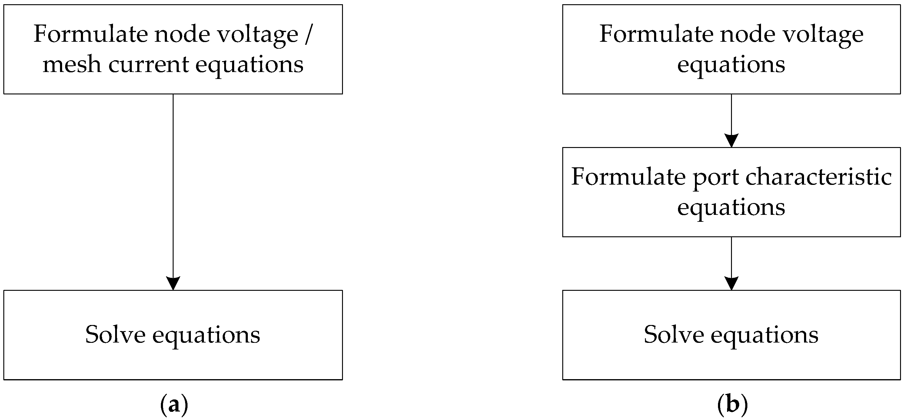
Figure 1a presents the overall process of the previous algorithms. It usually includes two steps: formulating node voltage or mesh current equations according to input data, and then solving the equations through numerical methods. Distinct from those, the PA inserts an additional step: converting the node voltage equations to port characteristic equations with the help of the Thévenin equivalent (see Figure 1b). This step concentrates efforts on train nodes instead of all nodes. Fewer variables need consideration than in the previous algorithms. In this section, the Thévenin equivalent and port characteristic equations are described first, then the equation-solving implementation is provided.
2.1. Thévenin Equivalent of Feeding Section
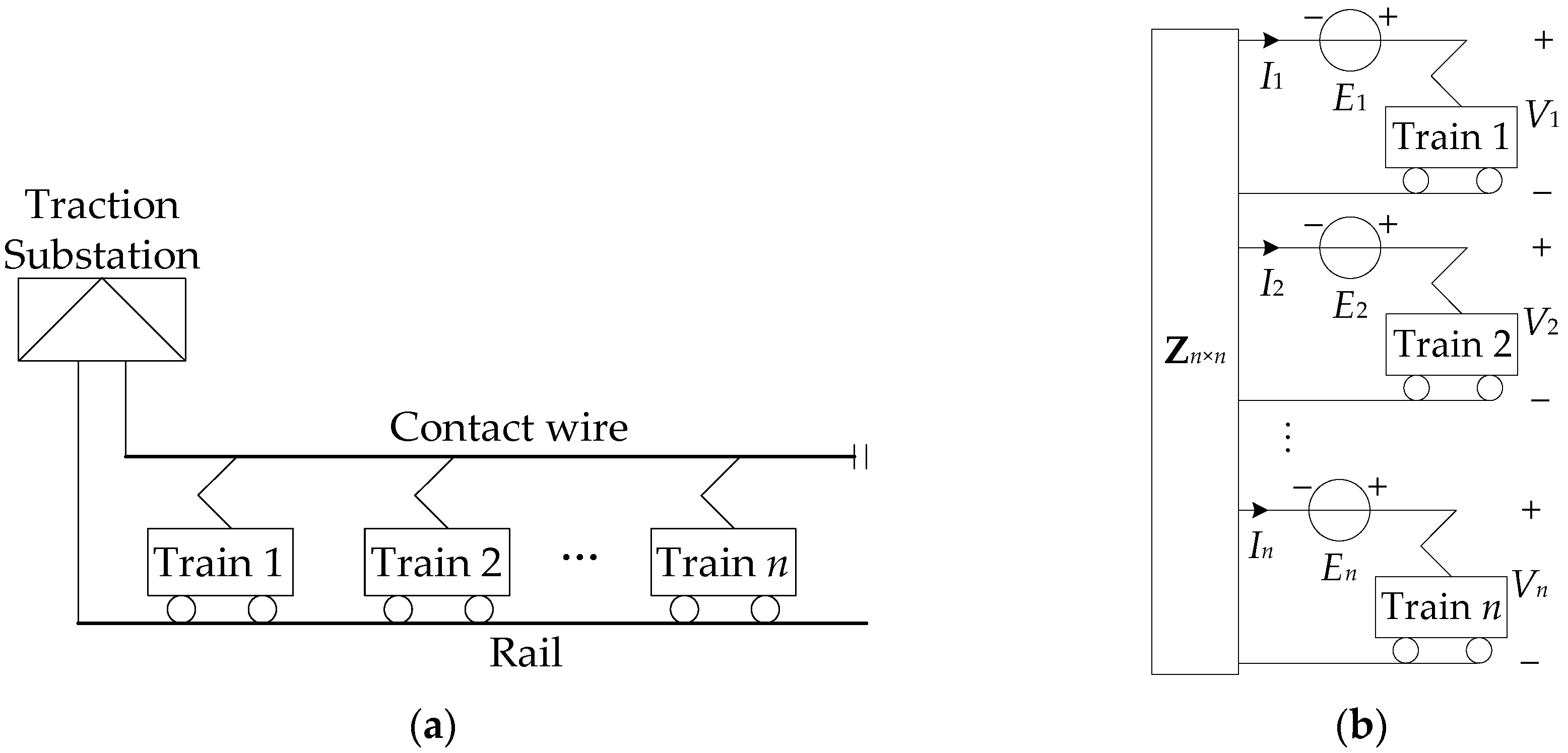
Figure 2 shows an independent feeding section which is a basic unit of a TPSS, and its Thévenin equivalent network, where Ei, Ii, and Vi stand for the open-circuit voltage, current, and voltage of port i, respectively. Z is the n × n impedance matrix of the equivalent network. The port characteristic equations are
where Zik represents the element in row i and column k of Z. The values of i and k are 1, 2, …, n, and will remain the same for the rest of this paper.
The critical task of the equivalence is to identify Ei and Zik. There are two equations derived from (1).
These two equations are employed to identify Ei and Zik as follows.
- Identification of Ei
- Set all train currents to 0 A.
- Solve node voltage equations.
- Ei equals the voltage of train i.
- Identification of Zik
- Set the current supplied by the substation to 0 A.
- Set the current of train k to −1 A, and that of the others to 0 A.
- Solve node voltage equations.
- Zik equals the voltage of train i.
2.2. Port Characteristic Equations Solving
If the complex power of train i is Pi + jQi, its voltage will be
Substituting (4) in (1) yields
The real form of (5) is
The subscript “Re” and “Im” denote the real and imaginary part of a complex number, respectively. Rik and Xik are the real and imaginary part of Zik, respectively. The Newton-Raphson method is exploited to solve (6) as follows:
- Set the initial value of the train current vectorAlternatively, set the initial values of the train voltages first, and then calculate the train currents.
- Calculate the residual vectorwhere
- Calculate the Jacobian matrixwhereThis step will not take much time since most elements are constant.
- Solve the corrective equationto obtain the corrective vector ∆I.J∆I = b
- If the norm of ∆I is smaller than a given value e, finish the calculation successfully. Otherwise, subtract ∆I from I and go to Step 6.
- If the number of iterations reaches a given value N, finish the calculation unsuccessfully. Otherwise, go to Step 2.
After they are determined, the values of the train currents are substituted into the node voltage equations to identify the node voltages. Afterwards, the power flow will be available easily. The flowchart of the PA is given in Figure 3.
3. Numerical Results
The convergence speed and ability to find multiple solutions of the proposed PA are analyzed through a numerical study with a comparison to the MNFA. All of the calculations are conducted on a desktop computer with an Intel Core i5-3470 CPU @ 3.20 GHz, 3.60 GHz and 8 GB memory.
3.1. Test System
Auto transformer (AT) feeding tends to be utilized in high-speed and heavy-haul railways due to its larger PSC than direct feeding. Therefore, realistic parameters of an AT feeding section are listed in Table 2 and adopted for the calculations.
3.2. Algorithm Properties
3.2.1. Convergence Speed
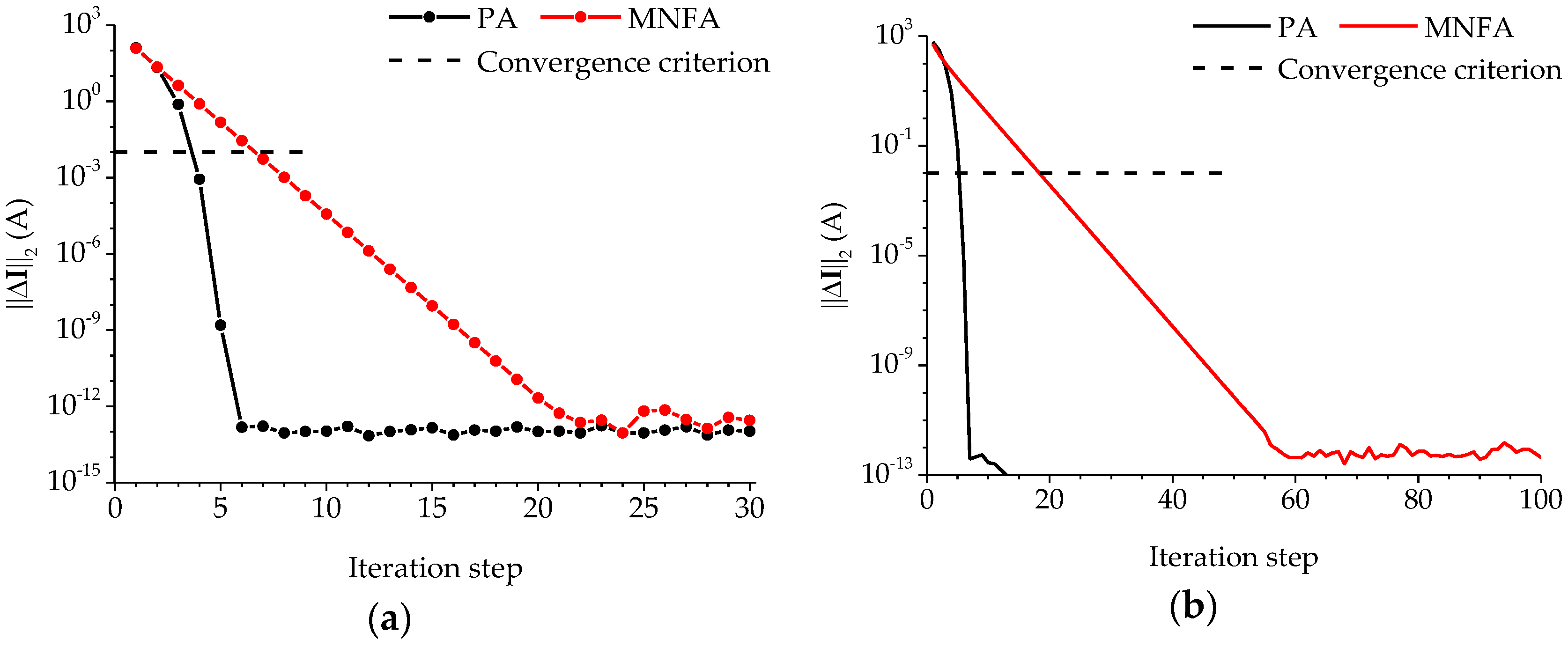
The train voltages calculated by the MNFA and PA are listed in Table 3 and Table 4, with the active power of each train set to 10 MW and 20 MW, respectively. The two sets of results are different, and the heavier the loads are, the larger the differences are. This is because the convergence speeds of the two algorithms contrast sharply, as illustrated in Figure 6. The fixed-point iteration used in the MNFA has linear convergence, while the Newton-Raphson method used in the PA has quadratic convergence. Hence, the PA requires a lower number of iterations to reach the convergence criterion.
Figure 7 presents the calculation speeds of the two algorithms. When the active power of each train ranges from 0 to 20 MW, the MNFA needs as much time as the PA to complete the calculation, roughly 85 ms, though the numbers of iteration are larger. However, as a reflection of the slow convergence, the number of iterations and the calculation time of the MNFA will rise to a great level if 20 MW is exceeded. In contrast, those of the PA are impacted slightly.
Most calculations are concentrated around the power limit during the RPF, so the substitution of the PA for the MNFA will save considerable time in a PSC assessment.
3.2.2. Ability to Find Multiple Solutions
If the initial values of the train voltages are set to 1 kV and the other conditions remain the same, the train voltages calculated by the PA will be lower, as listed in Table 5 and Table 6. Heavier loads result in smaller differences between the high and low voltage solutions. As to the MNFA, adequate initial values have not been found which bring convergence on the low voltage solutions.
PV curves are formed by the multiple solutions found under successively varying power, as shown in Figure 8. The PV curves are continuous in the neighborhood of the power limit, which proves that the PA did not encounter numerical difficulty. Moreover, most low voltage solutions are available only through the same set of initial values, simpler than the CPF. As a result, the programming is simplified significantly.
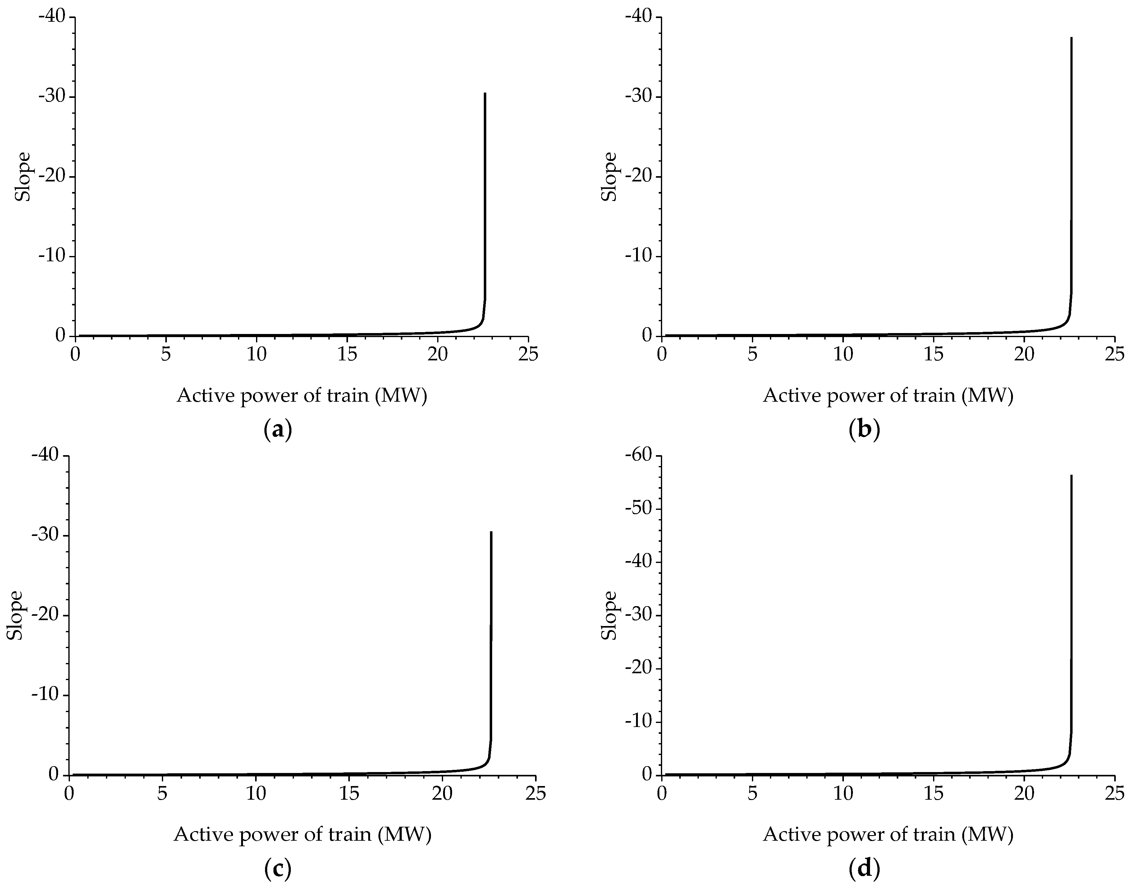
The MNFA is merely capable of the upper side of PV curves. Under these circumstances, the slope of the tangent line can be an auxiliary criterion of the power limit. It is concluded from Figure 8 that the slope is at negative infinity when the power limit is reached. Nonetheless, negative infinity is not available in the numerical calculations. Though a value can be selected to represent infinity, this approximation is not universal. Slopes of different trains are not equivalent, as presented in Figure 9. The selected value may not be appropriate for other trains or systems.
In summary, the PA can offer a more convincing proof of the power limit than the MNFA and an easier implementation than the CPF. The PA is more feasible to calculate the PSC.
4. Application to PSC Calculation
4.1. RPF Procedure
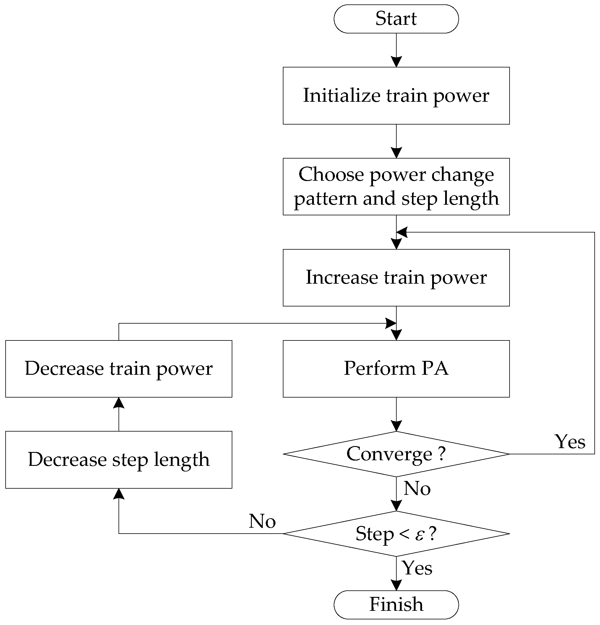
The lower side of a PV curve related to low voltage solutions may not have practical meaning, but it provides good verification of the power limit. It is known that the high and low voltage solutions approach while the power is increasing, and coincide when the power limit (4 × 22.602 MW = 90.408 MW for the test system) is reached [35]. If the power continues increasing, there will be no solutions. Therefore, the power limit found by the PA can represent the PSC. The RPF is performed based on the PA as follows:
- Set the complex power of each train to 0.
- Choose a load change pattern and step length, namely how much the complex power of each train increases or decreases.
- Increase the power according to the chosen pattern and step length.
- Perform the PA. If the calculation converges, go to Step 3. Otherwise, go to Step 5.
- If the step length is smaller than a given value ε, finish the calculation. Otherwise, go to Step 6.
- Decrease the step length, for instance, by half.
- Decrease the power according to the pattern and new step length, and go to Step 4.
Afterwards, the total active power of the trains is treated as the PSC. The process of power adjustment is illustrated in Figure 10, and the flowchart is given in Figure 11.
Although plenty of calculations were performed with the PA successfully, it is still not guaranteed that it can always converge near the power limit. In the case of a failure inferred from a discontinuous PV curve, the last solution on the curve can be used as the initial value of the next calculation, which is a kind of discrete continuation method [41].
4.2. Case Studies
The PSC can be enhanced through improving TPSS parameters and the organization of train operations. Enhancing the PSC through improving TPSS parameters includes connecting to a stronger public grid, employing AT feeding, or installing power factor correctors. Enhancing the PSC through the organization of train operations mainly affects the number and locations of trains. Both of them are effective, but the former is expensive and time-consuming. For that reason, the priority is given to the latter in order to realize the full potential of a present TPSS. Its effects are analyzed below.
4.2.1. Case 1
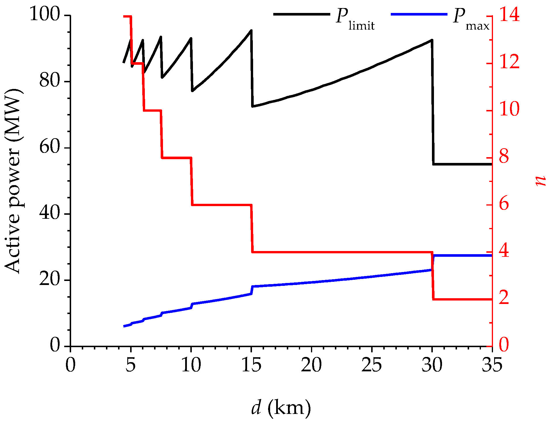
Suppose there are n trains in the test system, two of them are, respectively, at the section end on the up and down tracks, and the distance between adjacent trains d is the same, as depicted in Figure 12. Other conditions are identical to Section 3.1. The power limit Plimit and maximum active power of each train Pmax are influenced by d as presented in Figure 13. When n remains the same, Plimit rises with d increasing. When n becomes smaller, Plimit will fall steeply first, and then rise more gently than before. It has a minimum of 55.0 MW, and a maximum of 95.5 MW, varying acutely. As for Pmax, it rises slightly with the increment of d, and its maximum is 27.5 MW.
4.2.2. Case 2
If there are, respectively, two trains at the section start on the up track and the section end on the down track, as depicted in Figure 14, the results will be distinct. The minimum of Plimit has an increment to 89.7 MW, and the maximum is still 95.5 MW, as given in Figure 15a. The variation becomes not as severe as in Case 1. On the other hand, when n remains the same, Pmax almost keeps constant despite the change of d. Accordingly, Pmax is approximately inversely proportional to n, as shown in Figure 15b.
4.2.3. Discussion
The two cases above indicate how the organization of train operations affects the PSC. Plimit and Pmax in Case 1 are smaller than in Case 2 overall under the same number of trains. The reason is that the trains are closer to the section end, so that larger conductor impedance participates in the power transmission, and the TPSS supplies less power. Thus, it is recommended that trains on the up and down tracks not be concentrated near the section end, especially in weak TPSSs.
In addition, Plimit exceeds the rated capacity of the traction transformer considerably. The transformer does not match the PSC. If the PSC is expected to be fully utilized, the transformer capacity needs to be enlarged to 95.5 MW/0.97 ≈ 100 MVA at least.
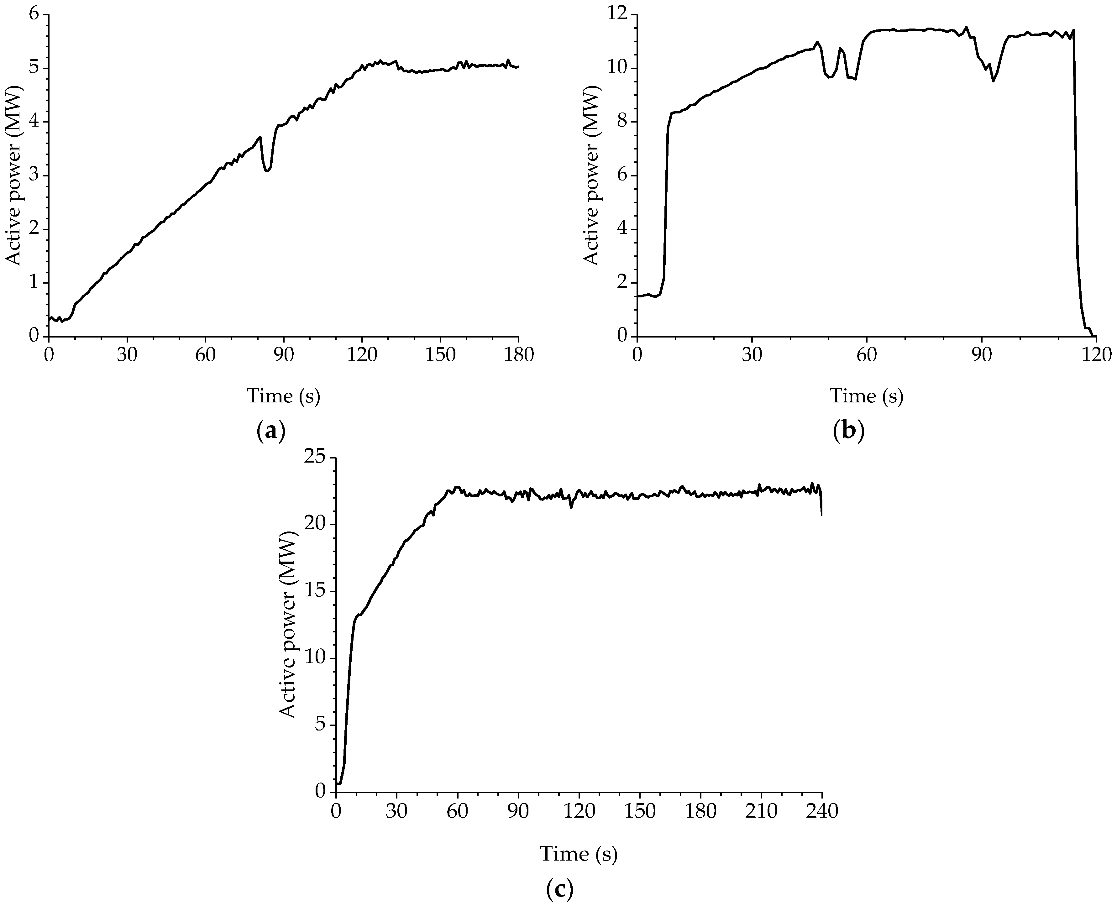
China EMUs in service can be classified into three levels according to the data of active power consumption, as given in Figure 16. Their minimum distance and time intervals corresponding to Case 1 and Case 2 are presented in Table 7, assuming that the speeds are 300 km/h. It is implied that the optimized organization of train operations is effective for the third level of EMUs, reducing the time interval by 1.4 min. If the opening hours are 16 h (6:00 to 22:00) a day, 100 pairs of trains more will be able to pass the feeding section, and the carrying capacity will be enhanced greatly, supposing that the signals and station facilities are able to cooperate with the power supply.
5. Conclusions
The PA is proposed for TPSSs based on the Thévenin equivalent. Port characteristic equations, converted from nodal voltage equations, are solved by the Newton-Raphson method. Owing to its quadratic convergence, the calculation time is shorter than the MNFA near the power limit. What is more, an easier approach to multiple solutions than the CPF is provided. The low voltage solutions can be found effortlessly only through another set of initial values, instead of knowledge of the numerical continuation and a complicated programming implementation. PV curves formed by multiple solutions are capable of providing vivid and visual information to TPSS planners and operators. With the help of the RPF based on the PA, the PSC is available conveniently.
The organization of train operations has significant effects on the PSC. It is recommended that the trains on the up and down tracks not be concentrated near the section end, especially in weak TPSSs. This optimization can help to shorten the interval of adjacent trains, and is beneficial to sufficient PSC utilization and enhancement of the carrying capacity.
Acknowledgments
This work was supported by the Fundamental Research Funds for the Central Universities (under Grant 2016YJS145) and the National Key Research and Development Program of China (under Grant 2017YFB1200802).
Author Contributions
Junqi Zhang and Mingli Wu conceived the algorithm. Junqi Zhang and Qiujiang Liu performed the calculations. Junqi Zhang analyzed the results and wrote the paper.
Conflicts of Interest
The authors declare no conflicts of interest.
References
- Gómez-Expósito, A.; Mauricio, J.M.; Maza-Ortega, J.M. VSC-based MVDC railway electrification system. IEEE Trans. Power Deliv. 2014, 29, 422–431. [Google Scholar] [CrossRef]
- Östlund, S. Rail power supplies going more power electronic. IEEE Electr. Mag. 2014, 2, 4–60. [Google Scholar] [CrossRef]
- Raygani, S.V.; Tahavorgar, A.; Fazel, S.S.; Moaveni, B. Load flow analysis and future development study for an AC electric railway. IET Electr. Syst. Transp. 2012, 2, 139–147. [Google Scholar] [CrossRef]
- Song, K.J.; Wu, M.L.; Agelidis, V.G.; Wang, H. Line current harmonics of three-level neutral-point-clamped electric multiple unit rectifiers: Analysis, simulation and testing. IET Power Electron. 2014, 7, 1850–1858. [Google Scholar]
- Zhao, N.; Roberts, C.; Hillmansen, S.; Nicholson, G. A multiple train trajectory optimization to minimize energy consumption and delay. IEEE Trans. Intell. Transp. Syst. 2015, 16, 2363–2372. [Google Scholar] [CrossRef]
- Wang, K.; Zhou, F.; Chen, J.Y.; Zhou, G.P. Capacity improvement based on power accommodation STATCOM for traction power supply. Electr. Power Autom. Equip. 2012, 32, 44–49. [Google Scholar]
- Battistelli, L.; Pagano, M.; Proto, D. 2 × 25-kV 50 Hz high-speed traction power system: Short-circuit modeling. IEEE Trans. Power Deliv. 2011, 26, 1459–1466. [Google Scholar] [CrossRef]
- Venikov, V.A.; Stroev, V.A.; Idelchick, V.I.; Tarasov, V.I. Estimation of electrical power system steady-state stability in load flow calculations. IEEE Trans. Power Appar. Syst. 1975, 94, 1034–1041. [Google Scholar] [CrossRef]
- Gravener, M.H.; Nwankpa, C. Available transfer capability and first order sensitivity. IEEE Trans. Power Syst. 1999, 14, 512–518. [Google Scholar] [CrossRef]
- Ou, Y.; Singh, C. Assessment of available transfer capability and margins. IEEE Trans. Power Syst. 2002, 17, 463–468. [Google Scholar] [CrossRef]
- Ou, Y.; Singh, C. Calculation of risk and statistical indices associated with available transfer capability. IEEE Proc. Gener. Transm. Distrib. 2003, 150, 239–244. [Google Scholar] [CrossRef]
- Zhang, S.; Cheng, H.; Zhang, L.; Bazargan, M.; Yao, L. Probabilistic evaluation of available load supply capability for distribution system. IEEE Trans. Power Syst. 2013, 28, 3215–3225. [Google Scholar] [CrossRef]
- Xu, S.; Miao, S. Calculation of TTC for multi-area power systems based on improved Ward-PV equivalents. IET Gener. Transm. Distrib. 2017, 11, 987–994. [Google Scholar] [CrossRef]
- Ho, T.K.; Chi, Y.L.; Wang, J.; Leung, K.K.; Siu, L.K.; Tse, C.T. Probabilistic load flow in AC electrified railways. IEEE Proc. Electr. Power Appl. 2005, 152, 1003–1013. [Google Scholar] [CrossRef] [Green Version]
- Pilo, E.; Rouco, L.; Fernández, A.; Hernández-Velilla, A. A simulation tool for the design of the electrical supply system of high-speed railway lines. In Proceedings of the IEEE 2000 Power Engineering Society Summer Meeting, Seattle, WA, USA, 16–20 July 2000. [Google Scholar]
- Wan, Q.Z.; Wu, M.L.; Chen, J.Y.; Wang, Z.J.; Liu, X.Y. Simulating calculation of traction substation’s feeder current based on traction calculation. Trans. China Electrotech. Soc. 2007, 22, 108–113. [Google Scholar]
- Aodsup, K.; Kulworawanichpong, T. Effect of train headway on voltage collapse in high-speed AC railways. In Proceedings of the Asia-Pacific Power and Energy Engineering Conference (APPEEC), Shanghai, China, 27–29 March 2012. [Google Scholar]
- Hill, R.J.; Cevik, I.H. On-line simulation of voltage regulation in autotransformer-fed AC electric railroad traction networks. IEEE Trans. Veh. Technol. 1993, 42, 365–372. [Google Scholar] [CrossRef]
- Ho, T.K.; Chi, Y.L.; Wang, J.; Leung, K.K. Load flow in electrified railway. In Proceedings of the Second International Conference on Power Electronics, Machines and Drives 2004 (PEMD 2004), Edinburgh, UK, 31 March–2 April 2004. [Google Scholar]
- Hsi, P.; Chen, S.; Li, R. Simulating on-line dynamic voltages of multiple trains under real operating conditions for AC railways. IEEE Trans. Power Syst. 1999, 14, 452–459. [Google Scholar]
- He, Z.Y.; Fang, L.; Guo, D.; Yang, J.W. Algorithm for power flow of electric traction network based on equivalent circuit of AT-fed system. J. Southwest Jiaotong Univ. 2008, 43, 1–7. [Google Scholar]
- Guo, D.; Yang, J.W.; He, Z.Y.; Zhao, J. Research on a flow analysis method of power supply system of AC high speed railway based on Newton method. Relay 2007, 35, 16–20. [Google Scholar]
- Goodman, C.J. Modelling and simulation. In Proceedings of the 4th IET Professional Development Course on Railway Electrification Infrastructure and Systems (REIS 2009), London, UK, 1–5 June 2009. [Google Scholar]
- Wu, M.L. Modelling of AC feeding systems of electric railways based on a uniform multi-conductor chain circuit topology. In Proceedings of the IET Conference on Railway Traction Systems (RTS 2010), Birmingham, UK, 13–15 April 2010. [Google Scholar]
- Wu, M.L. Uniform chain circuit model for traction networks of electric railways. Proc. CSEE 2010, 30, 52–58. [Google Scholar]
- He, J.W.; Li, Q.Z.; Liu, W.; Zhou, X.H. General mathematical model for simulation of AC traction power supply system and its application. Power Syst. Technol. 2010, 34, 25–29. [Google Scholar]
- Chen, H.W.; Geng, G.C.; Jiang, Q.Y. Power flow algorithm for traction power supply system of electric railway based on locomotive and network coupling. Autom. Electr. Power Syst. 2012, 36, 76–80. [Google Scholar]
- Hu, H.T.; He, Z.Y.; Wang, J.F.; Gao, S.B.; Qian, Q.Q. Power flow calculation for high-speed railway traction network based on train-network coupling systems. Proc. CSEE 2012, 32, 101–108. [Google Scholar]
- Zhi, H. Analysis of traction power supply capability for high-speed railway based on test data. High. Speed Railw. Technol. 2013, 4, 28–31. [Google Scholar]
- Wang, B.; Hu, H.T.; Gao, S.B.; Han, X.D.; He, Z.Y. Power flow calculation and analysis for high-speed railway traction network under regenerative braking. China Railw. Sci. 2014, 35, 86–93. [Google Scholar] [CrossRef]
- Ajjarapu, V.; Christy, C. The continuation power flow: A tool for steady state voltage stability analysis. IEEE Trans. Power Syst. 1992, 7, 416–423. [Google Scholar] [CrossRef]
- Iba, K.; Suzuki, H.; Egawa, M.; Watanabe, T. Calculation of critical loading condition with nose curve using homotopy continuation method. IEEE Trans. Power Syst. 1991, 6, 584–593. [Google Scholar] [CrossRef]
- Canizares, C.A.; Alvarado, F.L. Point of collapse and continuation methods for large AC/DC systems. IEEE Trans. Power Syst. 1993, 8, 1–8. [Google Scholar] [CrossRef]
- Chiang, H.; Flueck, A.J.; Shah, K.S.; Balu, N. CPFLOW: A practical tool for tracing power system steady-state stationary behavior due to load and generation variations. IEEE Trans. Power Syst. 1995, 10, 623–634. [Google Scholar] [CrossRef]
- Ejebe, G.C.; Tong, J.; Waight, J.G.; Frame, J.G.; Wang, X.; Tinney, W.F. Available transfer capability calculations. IEEE Trans. Power Syst. 1998, 13, 1521–1527. [Google Scholar] [CrossRef]
- Trias, A. The holomorphic embedding load flow method. In Proceedings of the 2012 IEEE Power and Energy Society General Meeting, San Diego, CA, USA, 22–26 July 2012. [Google Scholar]
- Rao, S.; Feng, Y.; Tylavsky, D.J.; Subramanian, M.K. The holomorphic embedding method applied to the power-flow problem. IEEE Trans. Power Syst. 2016, 31, 3816–3828. [Google Scholar] [CrossRef]
- Liu, C.; Wang, B.; Xu, X.; Sun, K.; Shi, D.; Bak, C.L. A multi-dimensional holomorphic embedding method to solve AC power flows. IEEE Access. 2017, 5, 25270–25285. [Google Scholar] [CrossRef]
- Basiri-Kejani, M.; Gholipour, E. Holomorphic embedding load-flow modeling of thyristor-based FACTS controllers. IEEE Trans. Power Syst. 2017, 32, 4871–4879. [Google Scholar] [CrossRef]
- Wang, B.; Liu, C.; Sun, K. Multi-stage holomorphic embedding method for calculating the power–voltage curve. IEEE Trans. Power Syst. 2018, 33, 1127–1129. [Google Scholar] [CrossRef]
- Ortega, J.M.; Rheinboldt, W.C. Iterative Solution of Nonlinear Equations in Several Variables; Academic Press: New York, NY, USA, 1970. [Google Scholar]
Figure 1.
Overall steps of algorithms. (a) Previous algorithms; (b) Port Algorithm (PA).

Figure 2.
Thévenin equivalent of feeding section. (a) Original feeding section; (b) Thévenin equivalent network.
Figure 2.
Thévenin equivalent of feeding section. (a) Original feeding section; (b) Thévenin equivalent network.

Figure 3.
Flowchart of PA.
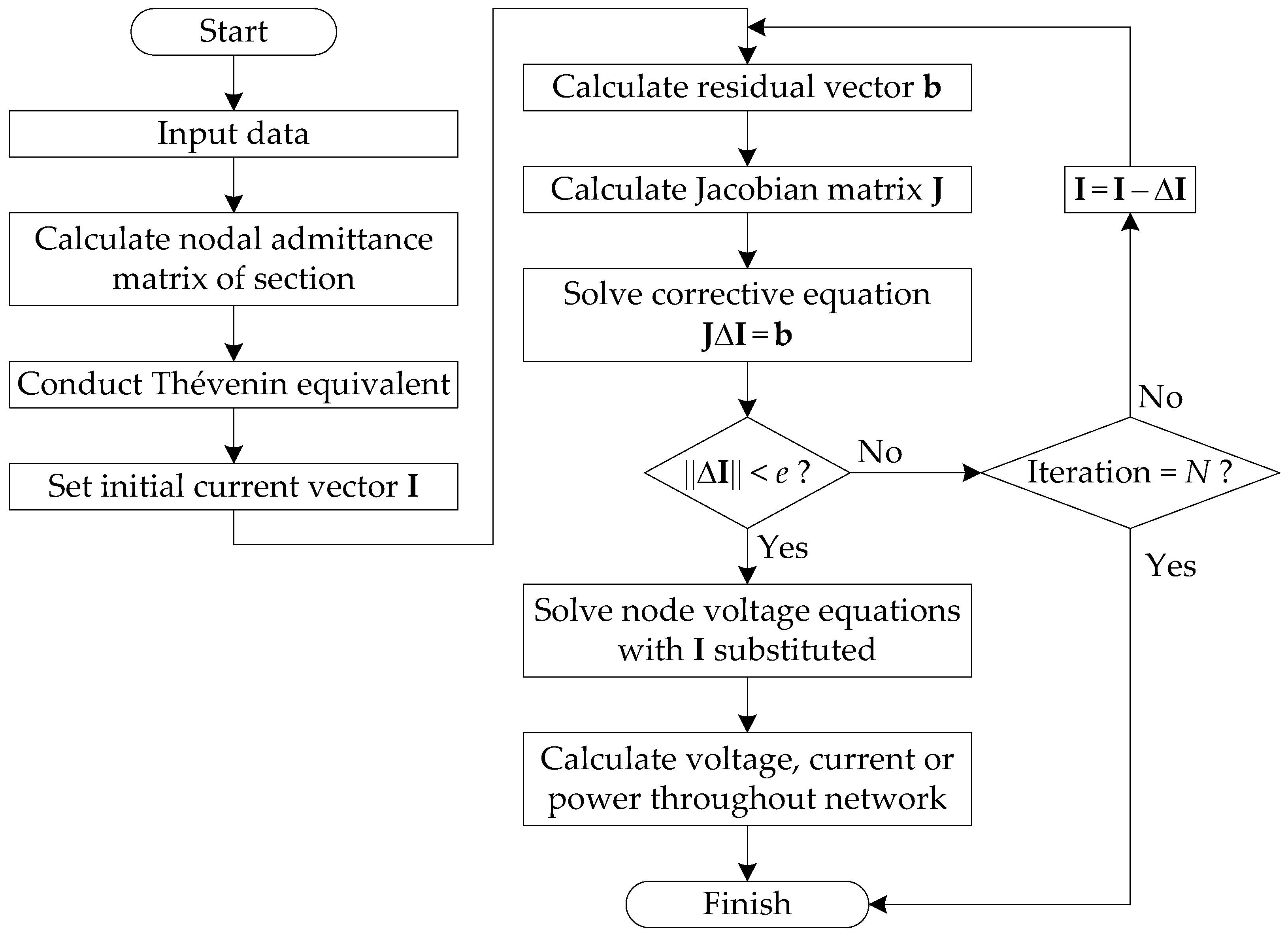
Figure 4.
Outline of test system.
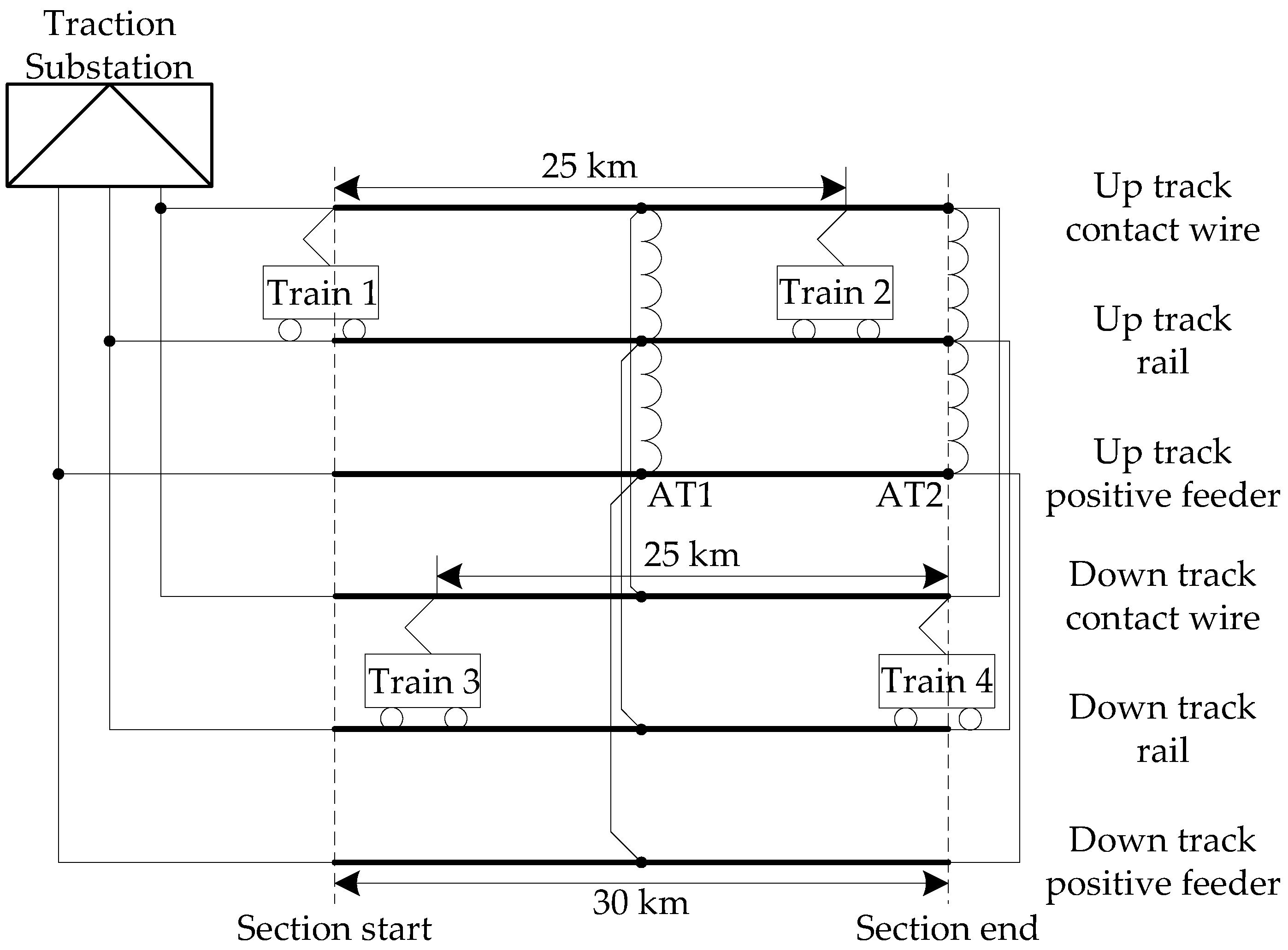
Figure 5.
Conductors in feeding section.

Figure 6.
Convergence speeds of two algorithms. (a) Light loads; (b) Heavy loads.

Figure 7.
Calculation speed of the two algorithms. (a) Number of iterations; (b) Calculation time.
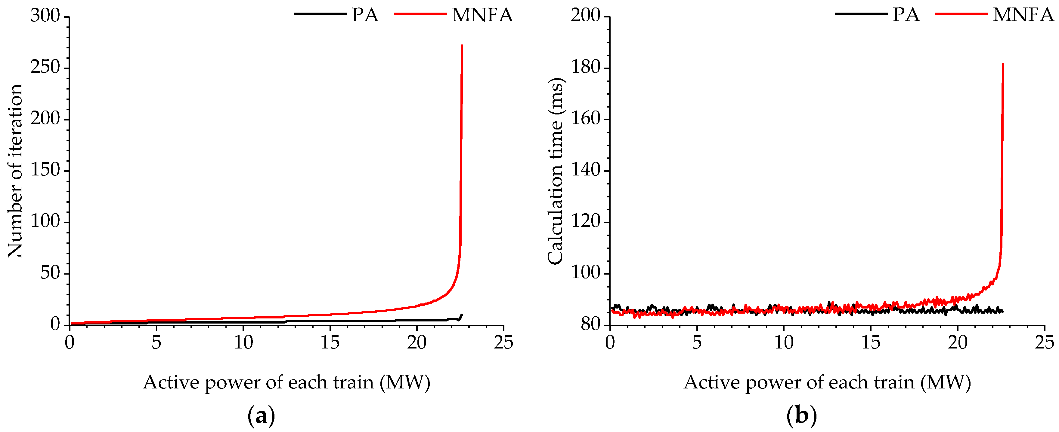
Figure 8.
Power-voltage (PV) curves of trains. (a) Train 1; (b) Train 2; (c) Train 3; (d) Train 4.
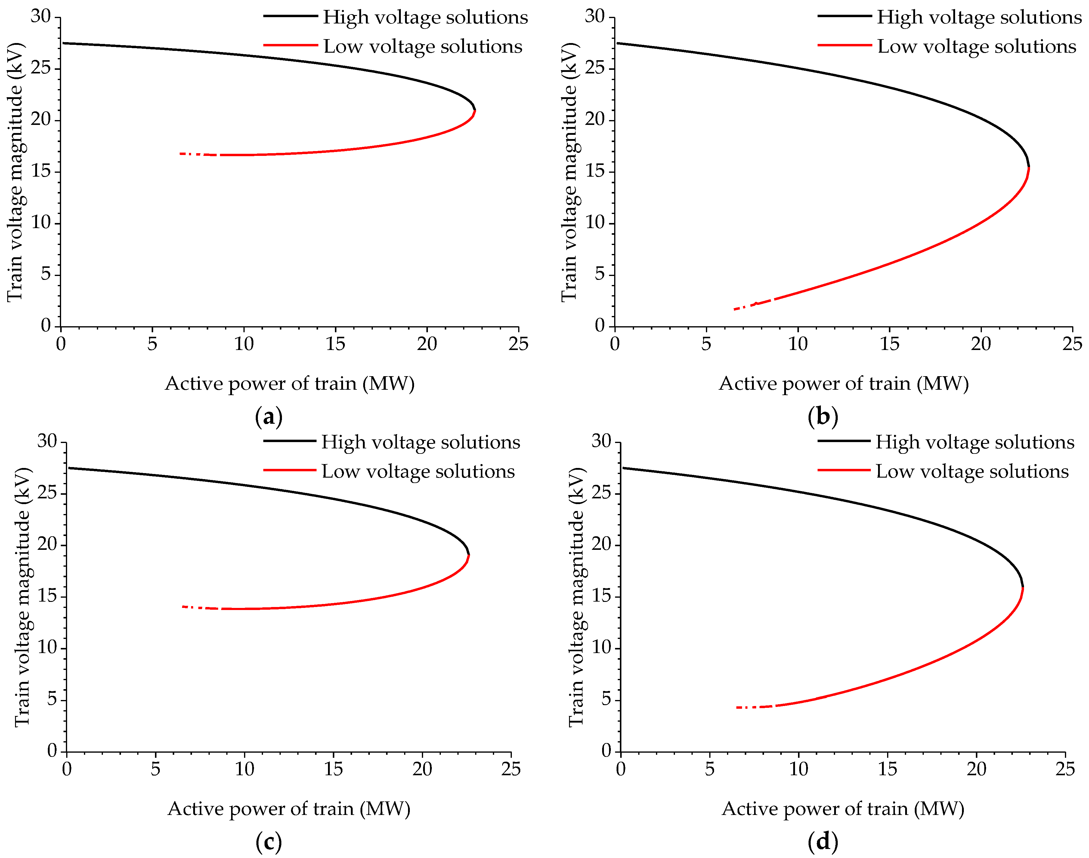
Figure 9.
Slopes of tangent lines of PV curves. (a) Train 1; (b) Train 2; (c) Train 3; (d) Train 4.

Figure 10.
Process of power adjustment.
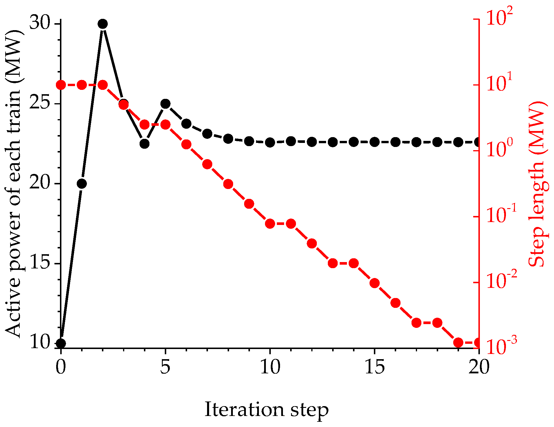
Figure 11.
Flowchart of repeated power flow (RPF).

Figure 12.
Location of successive trains in Case 1.
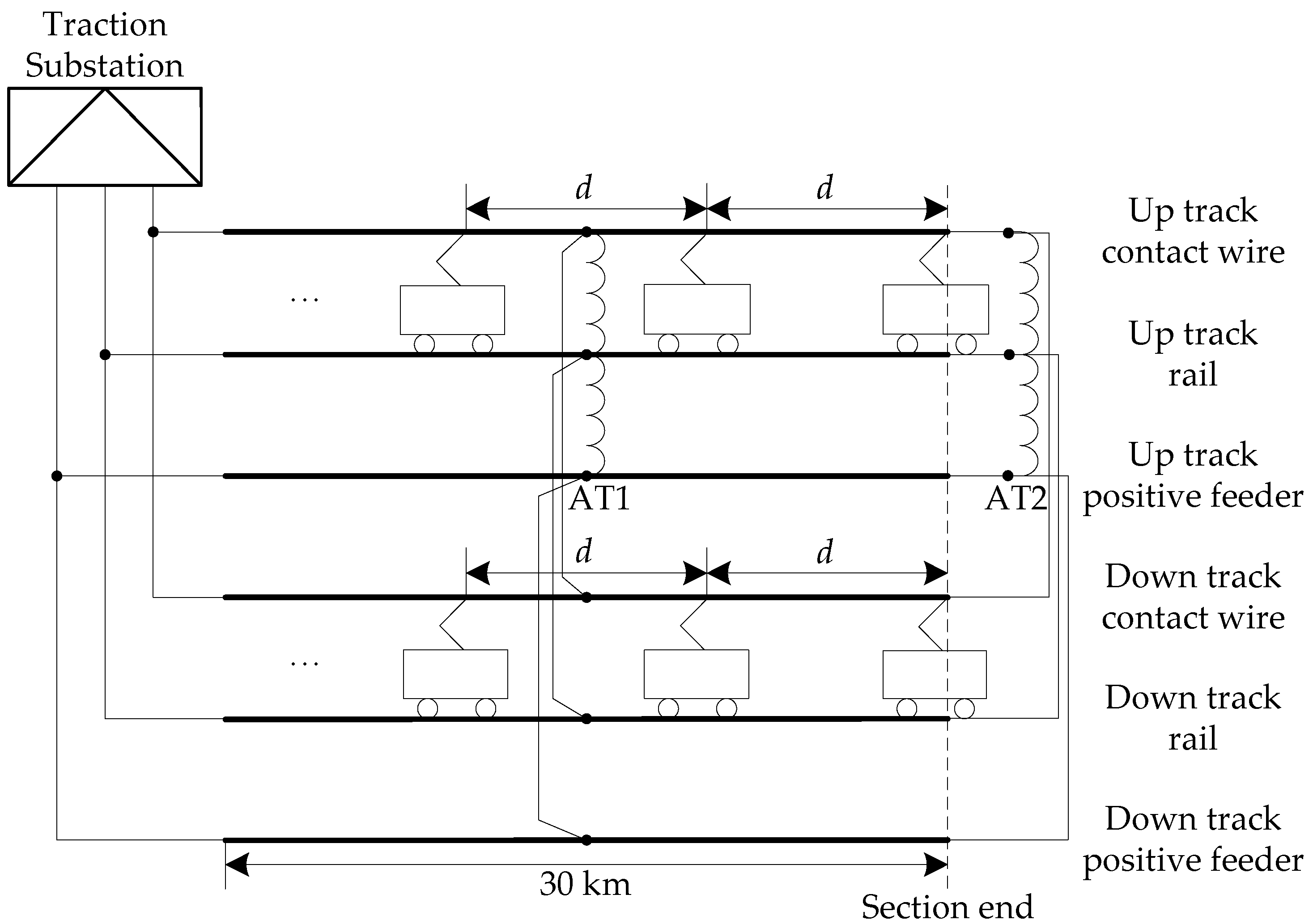
Figure 13.
Influence of d on Plimit and Pmax in Case 1.

Figure 14.
Location of successive trains in Case 2.
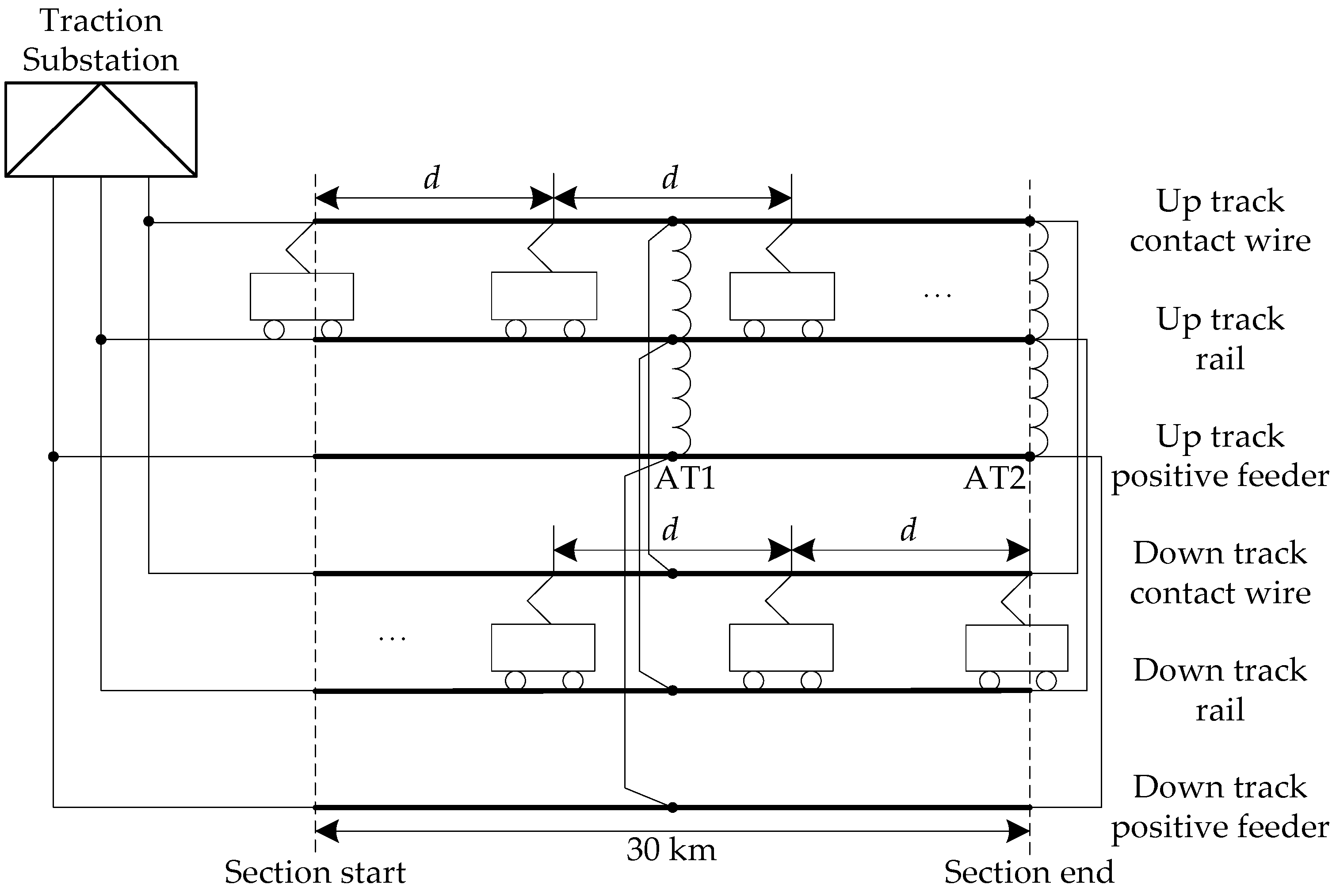
Figure 15.
Influence of d on Plimit and Pmax in Case 2. (a) Plimit and Pmax; (b) Curve fitting of the relation between Pmax and n.
Figure 15.
Influence of d on Plimit and Pmax in Case 2. (a) Plimit and Pmax; (b) Curve fitting of the relation between Pmax and n.
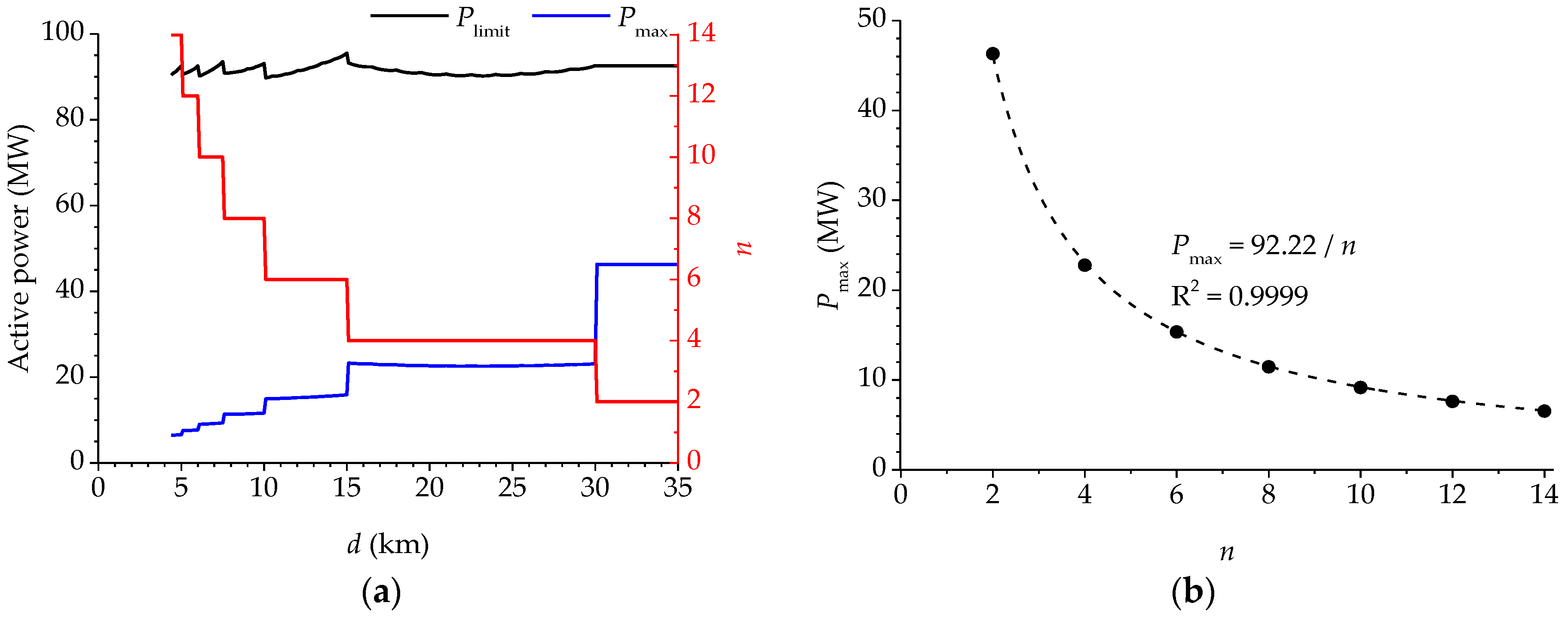
Figure 16.
Classification of active power consumption of China electric multiple units (EMUs). (a) Level 1, 5 MW; (b) Level 2, 10 MW; (c) Level 3, 20 MW.
Figure 16.
Classification of active power consumption of China electric multiple units (EMUs). (a) Level 1, 5 MW; (b) Level 2, 10 MW; (c) Level 3, 20 MW.

Table 1.
Features of traction power supply system (TPSS) power flow algorithms.
| Algorithm | Model Accuracy | Applicability to Feeding Scheme | Convergence Speed |
|---|---|---|---|
| [14] | Accurate | All | Linear |
| [15,16,17] | Accurate | All | Quadratic |
| [3,18,19,20,21] | Accurate | AT 1 feeding | Linear |
| [22] | Accurate | AT feeding | Quadratic |
| MNFA 2 | More accurate | All | Linear |
| PA | More accurate | All | Quadratic |
1 AT: auto transformer. 2 MNFA: Multiple conductor Nodal Fixed-point Algorithm.
Table 2.
Parameters of the test system.
| Parameter | Value |
|---|---|
| Section | |
| Track | 2 |
| Length | 30 km |
| Public grid | |
| System capacity | 5000 MVA |
| Voltage | 220 kV |
| Traction transformer | |
| Connection | single phase with secondary mid-point drawn out |
| Rated capacity | 40 MVA |
| Rated voltage | 220 kV/2 × 27.5 kV |
| Impedance | 8.4% |
| AT | |
| Location | 15 km and 30 km away from the substation |
| Leakage impedance | (0.1 + j 0.45) Ω |
| Trains | |
| Locations | as depicted in Figure 4 |
| Active power | the same value for all trains |
| Power factor | 0.97 lagging |
| Conductors | as depicted in Figure 5 |
| Rail to earth resistance | 100 Ωkm |
| Earth resistivity | 100 Ωm |
| Initial values of the train voltages | 40 kV |
| Convergence criterion | ‖∆I‖2 < 0.01 |
Table 3.
Train voltages calculated by MNFA and PA under light loads (Unit: V).
| Train | MNFA | PA | Difference |
|---|---|---|---|
| 1 | 26,162.81 − j 3049.25 | 26,162.79 − j 3049.25 | 0.02 |
| 2 | 24,639.93 − j 4664.22 | 24,639.89 − j 4664.22 | 0.04 |
| 3 | 25,585.18 − j 3666.87 | 25,585.15 − j 3666.87 | 0.03 |
| 4 | 24,784.16 − j 4552.74 | 24,784.12 − j 4552.74 | 0.04 |
Table 4.
Train voltages calculated by MNFA and PA under heavy loads (Unit: V).
| Train | MNFA | PA | Difference |
|---|---|---|---|
| 1 | 22,791.54 − j 6299.11 | 22,791.49 − j 6299.12 | 0.05 + j 0.01 |
| 2 | 18,037.97 − j 9100.00 | 18,037.88 − j 9099.99 | 0.09 − j 0.01 |
| 3 | 21,108.93 − j 7411.10 | 21,108.87 − j 7411.10 | 0.06 |
| 4 | 18,459.19 − j 8933.77 | 18,459.10 − j 8933.76 | 0.09 − j 0.01 |
Table 5.
Multiple solutions of train voltages under light loads (Unit: V).
| Train | High Voltage Solutions | Low Voltage Solutions | Difference |
|---|---|---|---|
| 1 | 26,162.79 − j 3049.25 | 15,959.64 − j 4789.04 | 10,203.15 + j 1739.79 |
| 2 | 24,639.89 − j 4664.22 | 1206.80 − j 3075.46 | 23,433.09 − j 1588.76 |
| 3 | 25,585.15 − j 3666.87 | 12,878.89 − j 5093.25 | 12,706.26 + j 1426.38 |
| 4 | 24,784.12 − j 4552.74 | 2848.02 − j 3879.99 | 21,936.10 − j 672.75 |
Table 6.
Multiple solutions of train voltages under heavy loads (Unit: V).
| Train | High Voltage Solutions | Low Voltage Solutions | Difference |
|---|---|---|---|
| 1 | 22,791.49 − j 6299.12 | 16,952.05 − j 7108.26 | 5839.44 + j 809.14 |
| 2 | 18,037.88 − j 9099.99 | 6071.67 − j 8086.42 | 11,966.21 − j 1013.57 |
| 3 | 21,108.87 − j 7411.10 | 13,760.17 − j 7954.93 | 7348.70 + j 543.83 |
| 4 | 18,459.10 − j 8933.76 | 6989.39 − j 8192.97 | 11,469.71 − j 740.79 |
Table 7.
Typical intervals of China EMUs.
| Level | Active Power Consumption | Minimum Interval in Case 1 | Minimum Interval in Case 2 |
|---|---|---|---|
| 1 | 5 MW | <5 km/<1 min | <5 km/<1 min |
| 2 | 10 MW | 7.5 km/1.5 min | 7.5 km/1.5 min |
| 3 | 20 MW | 22 km/4.4 min | 15 km/3 min |
© 2018 by the authors. Licensee MDPI, Basel, Switzerland. This article is an open access article distributed under the terms and conditions of the Creative Commons Attribution (CC BY) license (http://creativecommons.org/licenses/by/4.0/).
Share and Cite
MDPI and ACS Style
Zhang, J.; Wu, M.; Liu, Q. A Novel Power Flow Algorithm for Traction Power Supply Systems Based on the Thévenin Equivalent. Energies 2018, 11, 126. https://doi.org/10.3390/en11010126
AMA Style
Zhang J, Wu M, Liu Q. A Novel Power Flow Algorithm for Traction Power Supply Systems Based on the Thévenin Equivalent. Energies. 2018; 11(1):126. https://doi.org/10.3390/en11010126
Chicago/Turabian StyleZhang, Junqi, Mingli Wu, and Qiujiang Liu. 2018. "A Novel Power Flow Algorithm for Traction Power Supply Systems Based on the Thévenin Equivalent" Energies 11, no. 1: 126. https://doi.org/10.3390/en11010126
Note that from the first issue of 2016, this journal uses article numbers instead of page numbers. See further details here.