Simplified 1D Incompressible Two-Fluid Model with Artificial Diffusion for Slug Flow Capturing in Horizontal and Nearly Horizontal Pipes


1
Dipartimento di Ingegneria Meccanica ed Industriale, Università degli Studi di Brescia, Via Branze, 38, 25123 Brescia, Italy
2
Energy Resources Engineering, Stanford University, Stanford, CA 94305, USA
*
Author to whom correspondence should be addressed.
Energies 2017, 10(9), 1372; https://doi.org/10.3390/en10091372
Submission received: 31 July 2017
/
Revised: 1 September 2017
/
Accepted: 6 September 2017
/
Published: 10 September 2017
Abstract
:This article proposes a numerical resolution of a one-dimensional (1D), transient, simplified two-fluid model regularized with an artificial diffusion term for modeling stratified, wavy and slug flow in horizontal and nearly horizontal pipes. Artificial diffusion is introduced to prevent the unbounded growth of instabilities where the 1D two-fluid model is ill-posed. We propose a method to set the artificial diffusion case by case to obtain the desired cut-off at short wavelengths by combining the choice of the spatial discretisation and the amplification factors obtained by the linear stability analysis of the model. A proper criterion to simulate two-phase to single-phase flow transition, which occurs during slug formation, is also developed. Flow pattern transitions have been numerically computed and compared against theoretical transition boundaries and experimental observations. Moreover, we showed that the developed code computes slug initiation and slug characteristics, in a reasonably accurate way considering the simplicity of the model, comparing numerical results with well-known empirical correlations and experimental data. Furthermore, the model simplicity leads to a computationally-inexpensive numerical resolution; this can be useful in engineering applications where obtaining fast numerical results is fundamental, such as applications involving automated control for two-phase flows.
1. Introduction
Slug flow is a highly intermittent flow regime (liquid slugs are followed by large gas bubbles at a randomly fluctuating frequency [1,2]) typical of many engineering applications, such as petroleum transport pipelines, chemical and nuclear industries and buoyancy-driven fermentation devices [3]. This flow pattern may arise in horizontal and slightly inclined pipes from stratified flow because of the growth of instabilities: small perturbations appear on the liquid surface, and then, some may grow into larger waves to fill the pipe completely due to the well-known Kelvin–Helmholtz instability [4,5,6]. Slug flow can also be established due to pipe slope changes, i.e., when the pipe inclination, initially horizontal or downward, turns upward: in this case, the liquid accumulates because of gravity, and the liquid volume fraction increases until the stratified-slug flow transition occurs [7].
In the past few decades, many numerical codes have been developed to numerically describe slug flow and to compute slugs’ characteristics; one of the first methods was the ‘unit-cell’ approach, which enables a steady-state analysis of a control volume for gas bubbles and liquid slugs [8,9,10]. Issa and Kempf [11] pointed out that “unit-cell” models cannot predict flow pattern transitions; moreover, steady-state models are not necessarily capable of predicting slug flow initiation in inclined pipes due to liquid accumulation. More recently, transient models were developed, and they can be classified mainly into three categories. The first category includes the empirical slug specification method, which provides slug characteristics (length, shape, speed, growth and decay) using some ad hoc correlations, by assuming a priori that slug flow is already developed [12,13,14]. The second method is slug tracking: each single slug is tracked, i.e., the position of every slug tail and of every slug front is followed along the pipe using Lagrangian coordinates, and then, mass and momentum transport equations are solved at the slug front and tail. This approach was implemented in the commercial code OLGA, Oil and Gas simulator [15] and by Kjeldby et al. [16]. These two methods are able to compute slug flow characteristics, but they cannot simulate the transition from stratified to slug flow, since the slug flow regime is a priori assumed. The third method is slug capturing, introduced in [11]: the transient mono-dimensional two-fluid model set of equations and closure laws, which describe the stratified flow regime, are solved numerically, and slug formation is an automatic outcome of the computed flow. In fact, slug formation, growth and decay arise naturally from the numerical solution of the two-fluid model for stratified flow, without introducing special correlations or other constraints.
Most of the exposed techniques and the commercial simulators are based on cross-sectionally-averaged one-dimensional (1D) models combined with coarse grids [15,17] to fulfil the strict requirements on computational speed. Unfortunately, as often pointed out [18,19,20], the 1D two-fluid model is ill-posed under certain conditions. To partially overcome this issue, Issa and Kempf [11] used grid diffusivity to dampen the short wavelengths’ growth; this approach, however, does not ensure grid independence for every flow conditions since, as the grid is refined, the system is more sensitive to short wavelengths’ instabilities. Fullmer et al. [21] propose to consider the viscous stress term (i.e., Reynolds stress) in the momentum equation and to account for the surface tension (see also [22]); the latter approach does not have a straightforward implementation because of the third-order derivative. Again, it would be possible to render the system hyperbolic with a physically-meaningful term such as the virtual mass, but this kind of description was developed mainly for dispersed flow; thus, in this work, this is not a viable strategy because we focus mainly on stratified and slug flow regimes. Another way to overcome the unbounded short waves’ growth consists of adding some artificial diffusivity [23], introducing a second-order artificial diffusion term into the simplified two-fluid model, to obtain a formulation that provides convergent numerical solutions for flow conditions within the stratified and the stratified-wavy flow regime. Although the process of adding the artificial diffusivity in the numerical resolution of the simplified two-fluid model is not straightforward, we aim at exploring the possibility of this kind of regularization, which is based on sound mathematical principles: in fact, it has been demonstrated that if artificial axial diffusion is added to both mass and momentum equations, a cut-off wavelength is established below which all wavelengths are damped [23].
Afterwards, a transient roll-wave simulator based on a one-dimensional incompressible two-fluid model has been presented [24], together with a comparison of the numerical results with experimental data, showing good agreement; anyway, this approach does not take into account the slug flow regime because of the lack of a method to numerically describe the transition from two-phase to single-phase flow. In this work, instead, we developed a procedure to account for this phenomenon, which takes place when the liquid volume fraction tends to one as the slug body develops: this will extend the approach to slug flow.
The numerical description of the transition from two-phase to single-phase flow has been handled in very few papers, and at present, there is not fully consensual solution to cope with phase disappearance. Issa and Kempf [11] suggest to no longer solve the gas momentum equation and to set to zero the gas velocity when the gas volume fraction becomes negligible; however, they keep on solving the gas continuity equation, and when the gas volume fraction rises again above the prescribed threshold, the numerical solution of the momentum balance equation is re-introduced. Later, Nieckele et al. [25] followed this approach. Bonizzi et al. [26] introduced two thresholds to identify the transition from stratified to slug flow, one to observe when the gas volume fraction becomes small and one to observe the change of the volume fraction of the remaining gas, which must also be small. Zou et al. [27] give a special treatment of the momentum source terms if the volume fraction of the vanishing phase are lower than a certain value. Ferrari et al. [28] apply the approach by Issa and Kempf [11] to a five-equation two-fluid model, adopting a smoothing function between two thresholds and carefully handling the momentum source terms. Paillére et al. [29] describe an extension of the AUSM+scheme and propose to handle the velocity of the vanishing phase in a different way, if compared to [11]: they do not set the velocity arbitrarily to zero, but they make the vanishing phase velocity tend to the velocity of the remaining phase, thanks to a smoothing function. Cordier et al. [30] analyze the hyperbolicity of the two-fluid model and the loss of positivity of the numerical scheme in the presence of a vanishing phase.
The aforementioned transition criteria were developed for the four-equation two-fluid model [11,25,27,29], the five-equation two-fluid model [28], the six-equation two-fluid model [30] and the multi-field model [26]; as far as we know, no transition method has been developed for the case of a simplified two-fluid model, and thus, we develop here, for the first time, a completely new criterion for the two-equation model, on the basis of the previous literature.
Ansari and Shokri [31] developed a model to describe slug flow initiation, but its validity was restricted to the region of well-posedness of the two-fluid model: outside this region, the model is ill-posed, and the perturbation amplitude increases exponentially with decreasing mesh sizes. In the present paper, adopting a mathematical regularization, small wavelength instabilities are damped, and the model results in being well-posed.
In this paper, a simplified two-fluid model, regularized with artificial diffusion [23] is further developed introducing:
- a criterion to properly describe the transition from two-phase to single-phase flow (which is required when a slug forms);
- a method to choose the value of the artificial viscosity based on the fluid properties and flow rates, on the pipe geometry, on the space discretisation and on a desired cut-off wavelength; the latter is computed by solving the linear stability problem to dampen instabilities that possess a wavelength lower than a pipe diameter: this choice is coherent with the two-fluid model hypothesis, i.e., the resolution should not be lower than a representative length scale.
This paper is organized as follows: Section 2 presents the adopted simplified two-fluid model with artificial diffusion; Section 3 describes the numerical method, giving special care to the criterion developed to describe the transition from two-phase to single-phase flow. Section 4 shows the comparison of the numerical results with experimental data, when available, or with well-known empirical relations; finally, Section 5 reports some conclusions.
2. The Model
In this paper, we use a simplified version of the one-dimensional two-fluid model [23,32] for the derivation of the model. Similarly, in [33] and, more recently, in [34,35] and in [36], an analogous formulation of the two-equation two-fluid model is considered, which reduces the model from four to two equations.
The total mass conservation equation and the combined momentum equation for the stratified flow regime (see Figure 1) read:
where the subscripts l, g and i stand for the liquid phase, the gas phase and the interface, respectively. represents the phase volume fraction, the density, u the phase velocity, g the acceleration of gravity, the pipe inclination, assumed to be constant along the entire pipe, and h the liquid height; A denotes the pipe cross-sectional area, the shear stresses and s the wetted perimeters. In this work, both fluids are considered as incompressible, and the effect of surface tension is neglected.
The governing equations are completed by two algebraic relations: the volume fraction constraint, , and the relation between the superficial velocities and the mixture velocity, . The mixture velocity is an input parameter, which can be expressed as a function of time, and it is constant in space due to the incompressibility hypothesis. We considered the value of as constant throughout the simulation for the sake of simplicity, but nothing prevents it from being a time-dependent function.
The two-fluid model is well-posed only in the region where the Inviscid Kelvin–Helmholtz (IKH) criterion [33] expressed by Equation (3) (see Appendix B) is satisfied:
Since we are interested in the numerical description of slug flow, a regularization of the two-fluid model is required to prevent the unbounded growth of disturbances produced by small wavelengths’ amplification beyond the IKH boundary.
A numerical regularization is embodied within the model introducing a second-order tensor diffusion (i.e., artificial viscosity) in the mass and in the combined momentum equations—Equations (1) and (2)—to neutralize the short wavelengths that are not correctly described by the two-fluid model [23]. Even if the addition of artificial viscosity in both the mass and momentum equation may be physically questionable, it represents an acceptable compromise for engineering applications [37].
After including the artificial diffusion, the two-equation system becomes:
where is the flux:
and is the source term:
Closure relations for shear stresses are reported in Appendix A.
The vectors , and the matrix contain the liquid flow variables, the independent variables and the constant artificial viscosity:
This work focuses on the artificial viscosity to dampen instabilities at short wavelengths: thus, a method to set the element value of matrix is described in Section 4.1. Holmås [23] designed the matrix so that the initial value problem is well-posed for every flow condition ( must have real and positive eigenvalues), and all of the short wavelengths are stabilized. Coupling the artificial diffusion only to the liquid velocity in the momentum equation (0 m2/s) is not sufficient since, as the grid is refined, the short wavelengths grow bigger, and thus, numerical convergence is not achieved. The artificial diffusivity should be included also in the continuity equation and not only in the momentum equation [23], to obtain a cut-off wavelength under which all disturbances are damped. This approach aims at reproducing the regularization obtained by the surface tension description [18], and this can be achieved adopting a diagonal matrix, where both and have a positive value (namely, m2/s, m2/s and m2/s).
The method to choose the numerical viscosity values is discussed in Section 4.1: this reproducible method leads to a grid independent and regularized simplified two-fluid model for slug description; we aim at proposing a regularization that depends on flow and operative conditions and on physical considerations and that does not rely on an arbitrary choice of numerical viscosity values, as instead is done in [23].
3. Numerical Method and Two-Phase to Single-Phase Transition Modelization
In this section, we present the numerical method that has been embodied in an algorithm implemented in C language. In this work, the numerical method presented in [23] has been properly modified to account for the transition from two-phase to single-phase flow, which occurs during slug formation; we remark that, without this method, this approach would be applicable only in stratified and wavy flow and would be unable to describe slug flow; see Section 3.1. Moreover, boundary conditions have been consistently adapted to simulate a physical flow in pipelines.
First of all, the two-equation system, Equation (4), is split into an advection-source equation:
and into a diffusion equation:
to solve it with the second-order Strang operator splitting technique presented by [38]. A finite volume method and an explicit time discretisation have been adopted to solve Equation (8):
where the superscript n represents the time step, while the subscript j indicates the grid cell position. The FORCE (First-Order Centered) scheme by [39] has been adopted to discretize the numerical fluxes and :
Equation (11) states that each flux is computed as the mean of the fluxes obtained by the first-order Lax–Friedrichs method:
and by the second-order two-step Lax–Wendroff method:
where the predictor is:
The implementation of the FLIC (Flux-Limited Centered) scheme [39], a high-order extension of the FORCE scheme, is discussed in the Supplementary Material.
The diffusion equation, Equation (9), is solved with the implicit Crank–Nicholson scheme discussed in [40]: this method consists of the numerical solution of a linear equations system to obtain :
This set of linear equations has been solved using the linear algebra package within the GNU Scientific Library.
The algorithm adopts an adaptive time step, respecting the Courant–Friedrichs–Levy condition:
where is the maximum eigenvalue of the Jacobian of the advection equation, Equation (8), at time step n; the value of C has been set equal to 0.95 in all of the numerical results presented in Section 4, to obtain a large time step to optimize performances. When the liquid volume fraction is very close to one, the eigenvalues of the matrix , which does not include the artificial viscosity, turn imaginary: here, the time step is computed on the basis of the absolute value of the complex number. This choice ensures that the time step is smaller (and therefore safer) than the one computed on the basis of the real or of the imaginary part.
Boundary conditions are imposed in the following manner: velocity and volume fraction are extrapolated from the last cell at the outlet, while constant liquid superficial velocity and volume fraction are imposed at the inlet; at the beginning of the simulation, the liquid volume fraction and the velocity are assumed to be uniform along the pipe, representing a stratified smooth flow regime.
3.1. Two-Phase to Single-Phase Transition Criterion
During the slug onset process, the transition from two-phase flow to single-phase flow occurs: when this happens, the liquid volume fraction grows and tends to unity. Concerning the numerical simulations, if the liquid volume fraction value is not bounded or its growth not prevented, it becomes bigger than one, which is not physically acceptable. Moreover, if a proper numerical treatment of this phenomenon is not introduced, the simulation stops because the numerical fluxes cannot be computed. We need, therefore, to introduce a criterion to handle these numerical issues; as detailed in Section 1, only a few works have developed a similar treatment, and an ad hoc criterion for the simplified two-fluid model has not been proposed yet.
During the model development, we observed that, when the liquid volume fraction tends to one, the gas velocity required in the numerical fluxes of Equation (11) increases: this happens because of the small value of the denominator in the equation employed to compute from the mixture velocity, the liquid velocity and the liquid volume fraction:
Using this relation when leads to diverging values of , which are inserted in the numerical fluxes and, consequently, in the liquid velocity. This phenomenon has been observed by Zou et al. [27]: the velocity of the vanishing phase diverges and causes non-physical behaviors in the other variables. Our solution to prevent this phenomenon, due only to the numerics, consists of no longer computing gas velocity employing Equation (17) above the threshold , but forcing it to zero. Together with this, when the liquid volume fraction rises above the prescribed threshold (which was set equal to 0.999), also the hydrostatic term is removed from the combined momentum equation, since it is suitable just for two-phase flow. In addition, we set the interfacial friction and the gas-wall friction to zero, since the slug region contains only liquid. These adjustments prevent the uncontrolled growth of the gas velocity and help the liquid volume fraction stay bounded. Anyway, after the third step of the Strang operator splitting, a check on the value of the liquid volume fraction has to be performed, and if it exceeds the threshold value of 0.999, it is set to this value (a similar limitation on the volume fraction value is exposed in [27]). Thus, the idea is that when the liquid volume fraction exceeds a prescribed threshold, the terms concerning the gas phase are properly switched off to let the code manage slug formation or breakage. Since the numerical fluxes regarding the mass equation have not been modified by our criterion, the value of is free to evolve, and at the slug tail, it drops under the threshold: when this happens, gas velocity is computed using Equation (17), and the terms regarding the gas phase are reintroduced into the calculations.
Further information (the effect of the transition criterion on mass conservation, its validation by the water-air separation test [41]) is reported in the Supplementary Material.
4. Numerical Results
This section presents the results of the previously-described code, aiming at simulating slug flow in practical application. As pointed out earlier, the two-fluid model is able to predict slug growth and development in an automatic way, starting from uniform stratified flow as the initial condition. Thus, in this work, no perturbations are needed to initiate slug flow, since the adopted two-equation model descends from the two-fluid model itself.
We chose to present the results referring to two different pipe geometries to show that the code can be used to obtain predictions on real systems. The first configuration, which will be referred to as Pipe1, represents an experimental setup available in the Fisica Tecnica Laboratory at the University of Brescia, where many experiments have been performed in order to measure slug characteristics [42,43]. The second pipe configuration will be referred to as Pipe2 [11], whose geometrical properties and superficial velocity ranges are shown in Table 1. Both pipes are horizontal (i.e., ).
The adopted fluids are water and air, and their physical properties (density and viscosity) are reported in Table 2.
Slug initiation and slug characteristics will be discussed in both cases, and numerical results will be compared either with empirical models or with experimental results. Finally, the algorithm’s computational performance will be discussed.
4.1. On the Choice of the Artificial Viscosity Values
In this section, we will discuss the choice of the value of the elements and in the artificial viscosity matrix , Equation (7), adopted to regularize the simplified two-fluid model. In previous work [23], the values where arbitrarily set, i.e., and . Instead, we aim at providing a consistent method that can be applied for every flow condition; artificial viscosities are set case by case to obtain the desired cut-off at short wavelengths, and the choice is based on the analysis of the linear stability results. The two-fluid model is a one-dimensional averaged model: therefore, the assumption that the model resolution should not be lower than a representative length scale (i.e., the pipe diameter [37]) is consistent with the model hypothesis. The unbounded growth at short wavelengths is a consequence of the averaging process and of the absence of the surface tension description in the model; thus, numerical regularization aims at reproducing the small wavelengths’ cut-off.
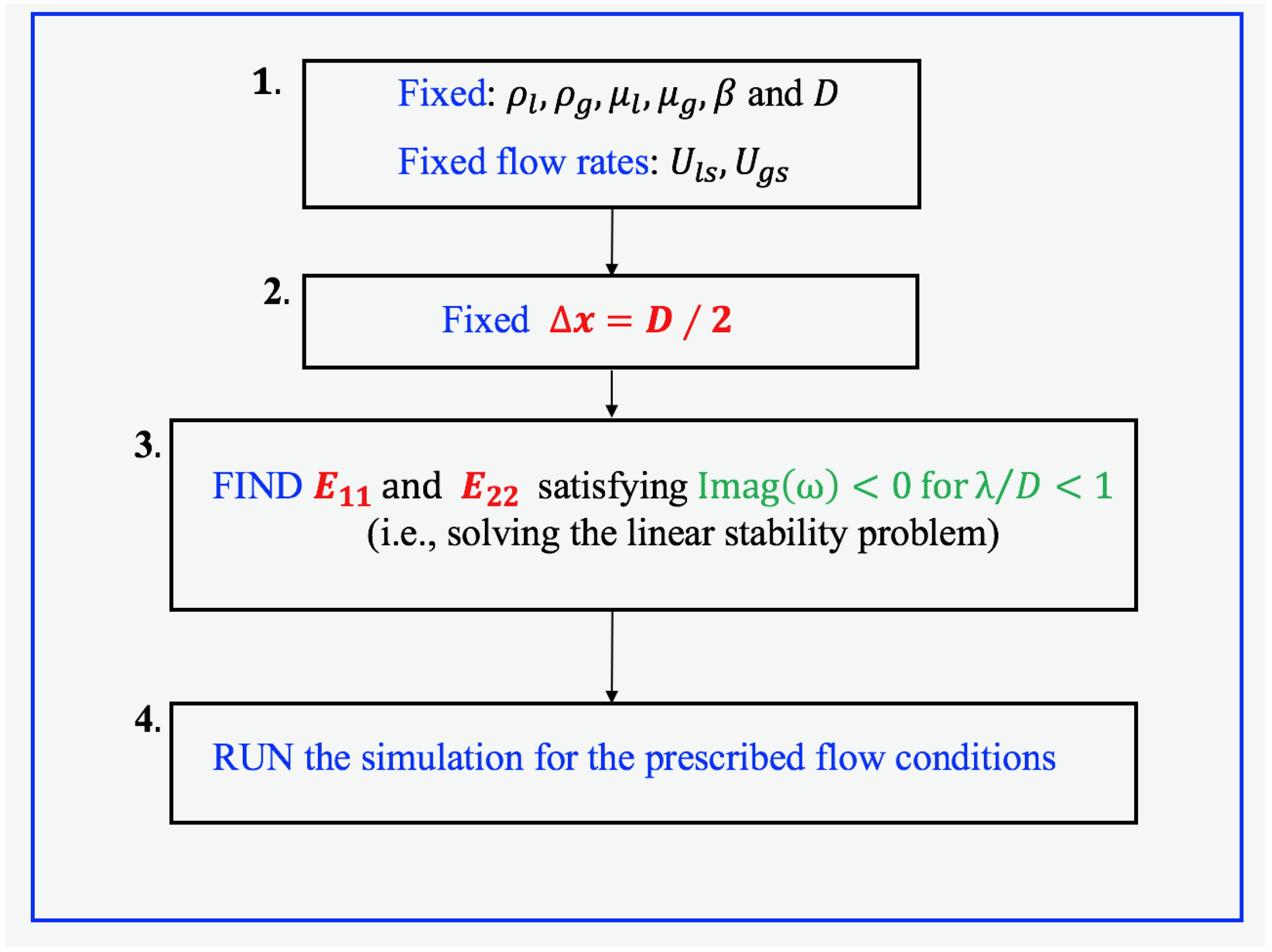
We used the results of the linear stability analysis to set the artificial viscosity values to obtain a cut-off wavelength of a representative pipe diameter, i.e., 0.022 mm in the case of Pipe1 and 0.078 mm in the case of Pipe2: the values of and are set so that the imaginary part of the amplification factor is lower than zero for wavelengths lower than a pipe diameter, i.e., Img() < 0 for . In Figure 2, the main steps of the algorithm are reported. In this way, we can obtain a well-posed model, and we set a lower cut-off to the size of perturbations allowed to grow in the case of unstable flow. Following the same approach proposed in [23], is set an order of magnitude lower than . The linear stability analysis is performed on the basis of the inlet superficial velocities, and the methodology is conceived of to provide an order of magnitude to the esteem of and , not a punctual value; thus, even if flow conditions along the pipe can differ from the inlet ones, the esteem provided by the proposed method is still acceptable.
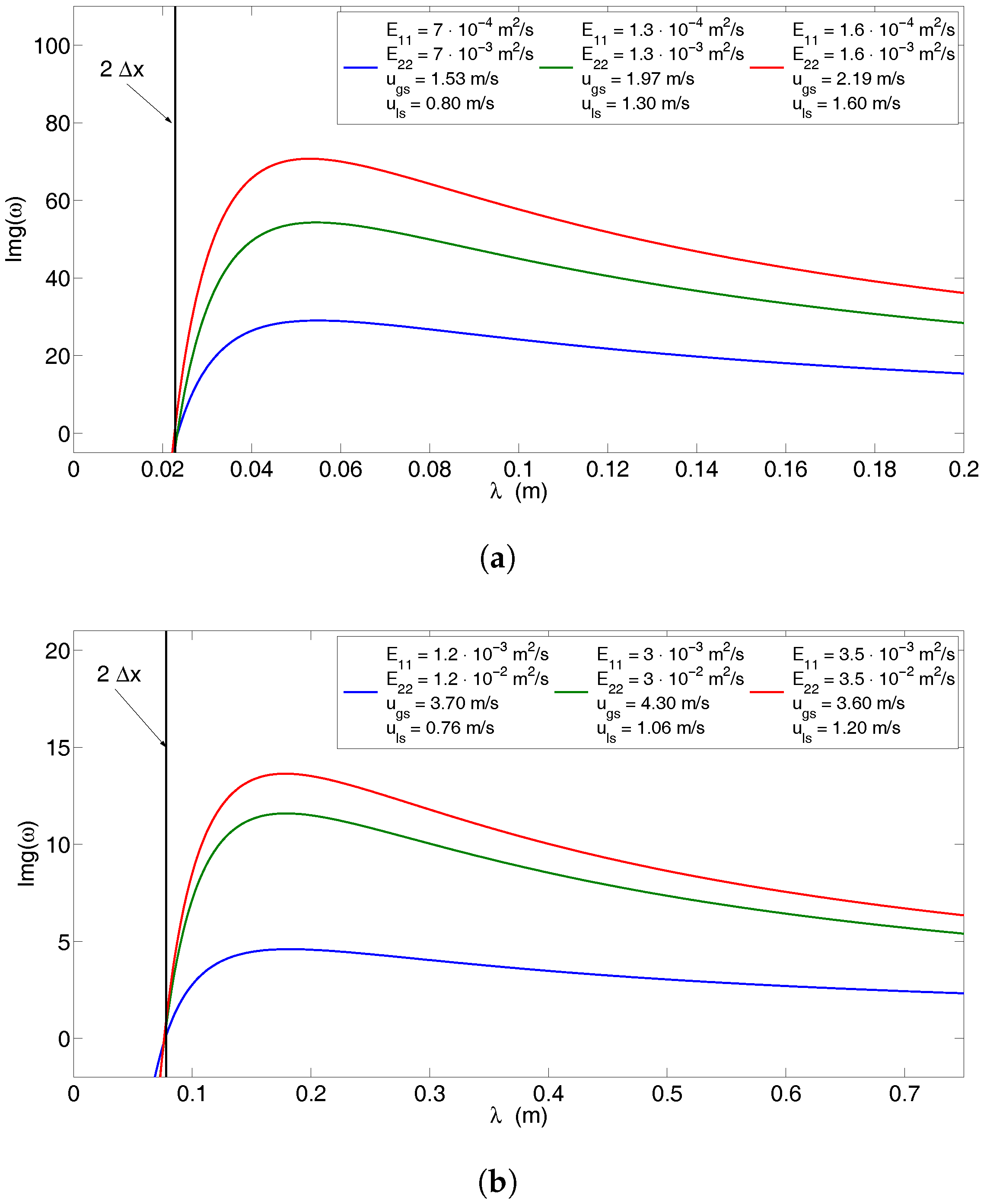
Figure 3 shows, for the investigated geometries and for different couples of superficial velocities, the amplification factor Img() as a function of the wavelength, which is defined as the imaginary part of the propagation velocity [23,33]. If Img() > 0, the corresponding wavelengths are amplified; if Img() < 0, they are damped. The values of and are the minima necessary to obtain a cut-off wavelength no higher than one pipe diameter, and they are specific for each couple of superficial velocities.
The presence of the spatial discretisation introduces additional numerical diffusivity: in Figure 3, at the left-hand side of the black vertical line, all of the waves with wavelengths smaller than x, where x = , are damped. Anyway, as previously discussed, artificial diffusivity must be included. Once the cut-off wavelength has been set at one pipe diameter, the spatial discretisation must be at least half the diameter of the pipe or smaller, since a wavelength of x is the smallest representable by a x grid. The independence of slug statistical characteristics from the spatial discretisation is shown in the Supplementary Material.
4.2. Flow Pattern Map and Code Validation
This section shows that the code is able to predict the transition between flow regimes (stratified and slug flow). Adopting the geometries described previously, several simulations were performed at different gas and liquid superficial velocities; for this purpose, the results of these simulations are plotted in Figure 4 and compared to flow transition boundary criteria. The Inviscid Kelvin–Helmholtz (IKH) boundary represents the transition between the well-posed and the ill-posed model (without including the artificial diffusivity) [33]: its points are the couples of superficial velocities that satisfy the equality in Equation (3).
The Viscous Kelvin–Helmholtz (VKH) line represents the linear stability boundary under the long wave approximation; see the Supplementary Material for details. The artificial viscosity becomes negligible under the long wave approximation, but as shown in [23], the diffusion does not affect in a sensible way the VKH line. Thus, the stability diagram is divided into three main regions, and the flow regimes can be placed on the flow pattern map in the following manner: under the VKH line, the flow is stratified smooth, since the VKH curve represents the border under which the smooth stratified flow is stable; above the IKH line, the flow pattern is slug flow, since here, we observe the unbounded wave growth; between the VKH and the IKH line, the flow can be stratified wavy or slug, since this is a transition region between the other two flow pattern regimes. Moreover, the dashed slanting line represents the couple of superficial velocity that has correspondent equilibrium hold up of 0.5: if the hold up is higher than 0.5, in the wavy region, there exists a higher probability that some waves may grow, completely fill the pipe section and generate slugs [44].
With the only purpose of better discerning the emerging flow regime, between stratified smooth and stratified wavy flow, numerical simulations were performed imposing a sinusoidal perturbation on the inlet volume fraction, respecting the following criteria:
- if the imposed perturbation was absorbed, the flow regime was classified as stratified smooth;
- if the perturbation was neither adsorbed, nor amplified until slug development, the emerging flow regime was wavy stratified;
- if the perturbation was amplified until the liquid completely filled the pipe, the slug flow regime was recognized.
Figure 4 shows that the code predicts the transition from stratified to wavy flow and from wavy to slug flow. It is possible to observe that, except for two points in Figure 4b, all of the smooth stratified results are under the VKH line, and then, before obtaining the slug flow regime, the transition to the wavy regime takes place; above the IKH line, the slug regime is obtained, as expected from theory.
In the Supplementary Material, a validation against the experimental flow pattern map reported in [45] is exposed.
4.3. Slug Characteristics
Several computations were carried out with different couples of superficial velocities for both geometries, with an end time of 300 s and a grid discretisation x = 0.256D to estimate slug characteristics, such as slug mean velocity, slug mean frequency and slug length. Results have been compared to experimental data, in the case of Pipe1, or with well-known empirical models, in the case of Pipe2, in order to validate numerical predictions. An analysis of the effect of the grid discretisation and of the threshold adopted in the transition from two-phase to single-phase flow (see Section 3) and a comparison against the slug initiation phenomenology proposed in Ansari [46] and in Ansari and Shokri [31] are reported in the Supplementary Material.
4.3.1. Slug Mean Velocity
Figure 5a shows, on the left, the comparison of the slug mean velocities obtained numerically by the two-equation model and the measured ones, for the geometry Pipe1, while Figure 5b compares slug computed translational velocities, in the case of Pipe2, and the predictions given by the relation reported in [47]; their correlation (, where is the distribution parameter and is the drift velocity) is for bubble velocity, but we adopted it under the hypothesis that the slug front moves at the same speed of the bubble before it; according to [47], we consider for turbulent flow (the case of this study) and for horizontal flow. In both the cases, the agreement between the numerical results and the experimental data (or empirical prediction) is satisfactory, since they are within the lines. Moreover, at the right-hand side of Figure 5a, we show that the computed slug velocities (black rings) follow accurately the trend predicted in [47] (blue line).
4.3.2. Slug Mean Frequency
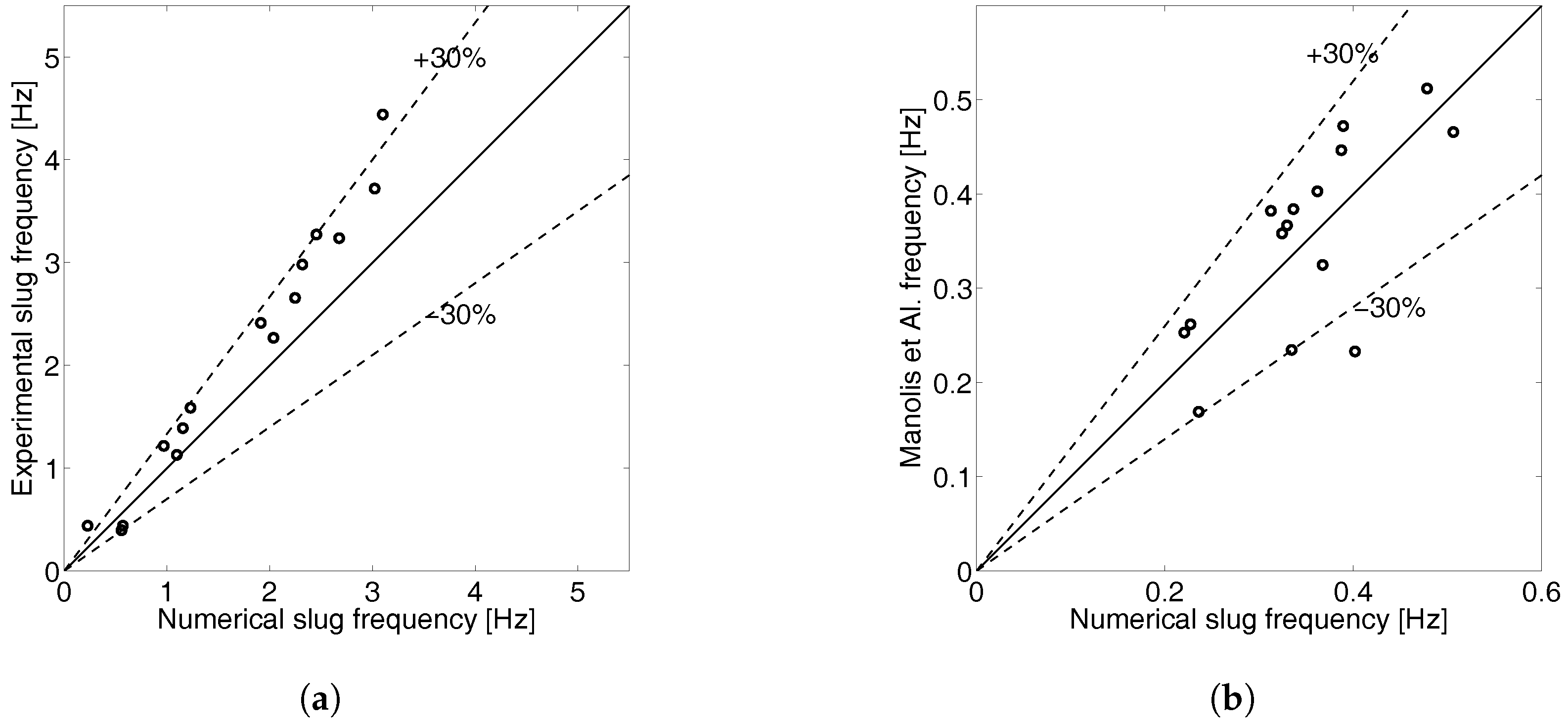
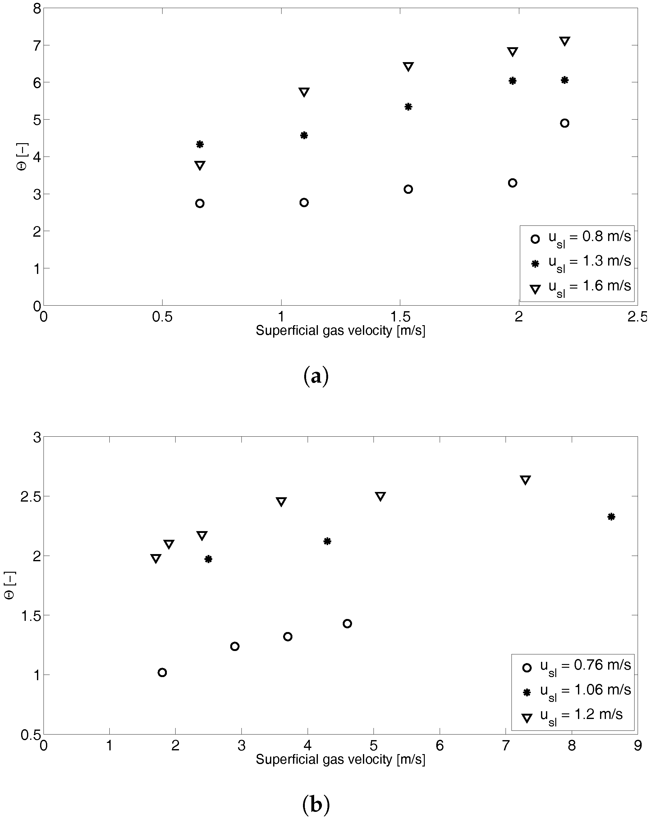
Slug mean frequencies computed on the Pipe1 geometry are compared in Figure 6a with the experimental results: the majority of the computed points are within or very close to the bound. For Pipe2, mean slug frequencies are reported in Figure 6b, where computed mean slug frequencies have been compared with the empirical correlation [48]: the slug frequencies computed with the two-equation model are in good agreement with this empirical correlation, and only a few points are out of the bounds. We can state that the numerical results compare quite well both with experimental data and with the proposed empirical correlation trend, since of the analyzed numerical results are in the bounds, in the case of Pipe1, and , in the case of Pipe2; however, the predictions are more accurate in the case of Pipe2, since in this case, of the analyzed results are within the bounds, while only in the case of Pipe1.
4.3.3. Slug Body Length Distribution
The computed slug body length distributions are reported in Figure 7: the typical log-normal distribution identified by experimental observation [49] is reproduced (the log-normal curves displayed in Figure 7 were fitted to the numerical data: the obtained mean and standard deviation are reported for each of the four cases). As concerns Pipe1, the experimental evidence indicates that the slug body lengths are typically in the range of 10–20-times the pipe diameter, while for Pipe2, the typical slug lengths are around 12–30 pipe diameters. In Figure 7a,b, we can see that the computed slugs are shorter than the ones observed experimentally, but that the statistical behavior of the distribution is preserved.
The discrepancy between the computed slug lengths and the experimental ones could be due to the simple closure laws adopted in this work, because they do not describe faithfully the physical process that makes the slugs grow, that is the liquid slug deceleration given by the liquid-wall shear stresses. Moreover, in this model, the gas entrainment is not taken into account, and this also plays a crucial role in the slug development.
4.4. Computational Performances
In this paragraph, the computational performances of the presented algorithm will be briefly discussed, with the purpose of giving to the reader the possibility to compare the performance of the presented code with the ones of other numerical simulators. Several numerical tests have been performed with many couples of superficial velocities, all of them with and en time of 300 s and a grid discretisation x = . All of the simulations were performed serially on an Intel Xeon CPU, 2.30-GHz processor. To show the computational performances of the code on this machine, we define the ratio between the computational time and the simulated time:
If the parameter is lower than one, the simulation runs faster than real time.
Figure 8a,b shows the dimensionless computational time resulting from simulation respectively for Pipe1 and Pipe2; as we can see, keeping the liquid superficial velocity constant, the simulation time grows almost linearly, except for some points, as the superficial gas velocity increases: this velocity-dependent simulation time is due to the adaptability of the time step on the basis of the eigenvalues, which are strongly related to the phases velocities; as the phase velocities increases, also the eigenvalues grow, and this leads to smaller time steps; smaller time steps mean that more computational iterations are needed to reach the desired end time, and thus, a higher computational time is required.
Although the computational time is very case specific, depending on the pipe length, on the grid discretisation and on the flow rates, the code shows promising computational performances if we evaluate the computational time of the presented example cases. Moreover, to further improve the computational efficiency, it would be possible to run the code in parallel: the conversion from a serial to a parallel architecture can be done, for example, using the domain decomposition method and the OpenMP API. The algorithm consists of dividing the pipe domain into N chunks, and the numerical resolution of each chunk is assigned to a thread. The chunk-thread assignment and the exchange of information among the threads (fundamental to send and receive boundary conditions) can be done using the features available in the OpenMP API. Once each thread has finalized a time iteration on the assigned chunk, boundary conditions are exchanged with the neighboring threads, and the subsequent iteration can take place. When the desired end time has been reached, the solution is reconstructed from the N solutions. As concerns practical applications, such as the preliminary design of the operative setup, where fast predictions are required, this code can be a a reliable tool for this kind of purpose.
5. Conclusions
In this work, a numerical code for slug capturing in a horizontal pipe was developed and implemented. We adopted a simplified two-fluid model regularized with artificial diffusion, to deal with the issue of ill-posedness. An original numerical procedure to describe the two-phase to single-phase flow transition was designed and implemented, thanks to which the numerical code is able to simulate the slug flow regime, as well as smooth and wavy stratified flow. A consistent choice of the coefficients of the artificial diffusion matrix was proposed, which depends on the pipe configuration, as well as inlet flow rates.
The numerical algorithm was tested on two different pipe geometries and validated against experimental results; it was shown that the obtained numerical results agree well with experimental data and with well-known empirical correlations. The developed simulator was proven able to describe in a satisfactory way the transitions between flow regimes (i.e., stratified smooth, stratified wavy and slug) and to compute well slug characteristics, especially mean frequency and mean velocity. As concerns slug lengths, the experimentally-observed log-normal distribution clearly emerges from the numerical results, but the computed mean length is underestimated: this could be because of the simple form of the adopted closure laws and the omission of gas entrainment; these issues should be, in our opinion, addressed in further works.
Finally, the computational performances of the code were discussed, showing that the simplicity of the model leads to a computationally-inexpensive resolution: this feature and the possibility of a straightforward conversion of the algorithm on a parallel architecture render the proposed simulator as a good candidate for applications where fast predictions are required.
Supplementary Materials
Supplementary materials can be found at www.mdpi.com/1996-1073/10/9/1372/s1. The Supplementary Material reports further information on the numerical method, validation against an experimental flow pattern map, effect of grid refinement and threshold variation on slug characteristics, comments on slug initiation and details on the VKH boundary.
Author Contributions
Arianna Bonzanini developed the code, tested it, obtained the numerical results and wrote the paper. Davide Picchi developed the method to esteem the artificial viscosity by linear stability analysis, suggested the comparison of numerical results against flow pattern maps and contributed to writing and revising the paper. Pietro Poesio supervised the work, contributed to the theory and modeling and to revising the paper.
Conflicts of Interest
The authors declare no conflict of interest.
Appendix A. Shear Stresses Model
Interfacial and wall shear stresses are modeled using single-phase friction relations based on the phase hydraulic diameter [50]. Single-phase closure relations are sufficiently accurate for turbulent phases in two-phase flow [51], and it would have been inappropriate to adopt complex and elaborated closure laws, considering the simplicity of the model. Thus, the following relations for shear stresses, at the wall and at the interface, respectively, have been adopted (for fluid ):
Friction factors are computed as:
The Reynolds number is:
where the hydraulic diameters of liquid and gas phase are, respectively:
Geometrical variables appearing in these equations can be found in Figure 1.
Appendix B. Matrices Coefficients
Holmas [23] rewrote the two-equation two-fluid model in the following quasi-linear form:
We report here the coefficients of the matrix and , adopted in the model. The entries not reported below are zero.
with .
References
- Fabre, J.; Liné, A. Modeling of two-phase slug flow. Ann. Rev. Fluid Mech. 1992, 24, 21–46. [Google Scholar] [CrossRef]
- Woods, B.D.; Hurlburt, E.T.; Hanratty, T.J. Mechanism of slug formation in downwardly inclined pipes. Int. J. Multiph. Flow 2000, 20, 63–79. [Google Scholar] [CrossRef]
- Dukler, A.E.; Fabre, J. Gas-liquid slug flow-knots and loose ends. In Proceedings of the 3rd International Workshop Two-phase Flow Fundamentals, London, UK, 15–19 June 1992. [Google Scholar]
- Kordyban, E.S. Some details of developing slugs in horizontal two phase flow. AIChE J. 1985, 31, 802–806. [Google Scholar] [CrossRef]
- Lin, P.Y.; Hanratty, T.J. Prediction of the initiation of slugs with linear stability theory. Int. J. Multiph. Flow 1986, 12, 79–98. [Google Scholar] [CrossRef]
- Fan, Z.; Ruder, Z.; Hanratty, T.J. Pressure profiles for slugs in horizontal pipes. Int. J. Multiph. Flow 1993, 19, 421–437. [Google Scholar] [CrossRef]
- Jansen, F.E.; Shoham, O.; Taitel, Y. The elimination of severe slugging. Int. J. Multiph. Flow 1996, 22, 1055–1072. [Google Scholar] [CrossRef]
- Wallis, G.B. One-Dimensional Two-Phase Flow; McGraw-Hill: New York, NY, USA, 1969. [Google Scholar]
- Dukler, A.E.; Hubbard, M.G. A model for gas-liquid slug flow in horizontal and near horizontal tubes. Ind. Eng. Chem. Fundam. 1975, 14, 337–347. [Google Scholar] [CrossRef]
- Taitel, Y.; Barnea, D. Two-phase slug flow. Adv. Heat Transf. 1990, 20, 83–132. [Google Scholar]
- Issa, R.I.; Kempf, M.H.W. Simulation of slug flow in horizontal and nearly horizontal pipes with the two-fluid model. Int. J. Multiph. Flow 2003, 29, 69–95. [Google Scholar] [CrossRef]
- De Henau, V.; Raithby, G.D. A transient two-fluid model for the simulation of slug flow in pipelines—I. Theory. Int. J. Multiph. Flow 1995, 21, 335–349. [Google Scholar] [CrossRef]
- De Henau, V.; Raithby, G.D. A transient two-fluid model for the simulation of slug flow in pipelines—II. Validation. Int. J. Multiph. Flow 1995, 21, 351–363. [Google Scholar] [CrossRef]
- Fagundes Netto, J.R.; Fabre, J.; Peresson, L. Shape of long bubbles in horizontal slug flow. Int. J. Multiph. Flow 1999, 25, 1129–1160. [Google Scholar] [CrossRef]
- Bendiksen, K.H.; Malnes, D.; Moe, R.; Nuland, S. The dynamic two-fluid model OLGA: Theory and application. SPE Prod. Eng. 1991, 6, 171–180. [Google Scholar] [CrossRef]
- Kjeldby, T.K.; Henkes, R.A.W.M.; Nydal, O.J. Lagrangian slug flow modeling and sensitivity on hydrodynamic slug initiation methods in a severe slugging case. Int. J. Multiph. Flow 2013, 53, 29–39. [Google Scholar] [CrossRef]
- Pauchon, C.; Dhulesia, H.; Lopez, D.; Fabre, J. TACITE: A comprehensive mechanistic model for two-phase flow. In Proceedings of the 6th International Conference on Multiphase Production, Cannes, France, 16–18 June 1993. [Google Scholar]
- Ramshaw, J.D.; Trapp, J.A. Characteristics, stability, and short-wavelength phenomena in two-phase flow equation systems. Nucl. Sci. Eng. 1978, 66, 93–102. [Google Scholar] [CrossRef]
- Barnea, D.; Taitel, Y. Non-linear interfacial stability of separated flow. Chem. Eng. Sci. 1994, 49, 2341–2349. [Google Scholar] [CrossRef]
- Louaked, M.; Hanich, L.; Thompson, C.P. Well-posedness of incompressible models of two- and three-phase flow. IMA J. Appl. Math. 2003, 68, 595–620. [Google Scholar] [CrossRef]
- Fullmer, W.D.; Ransom, V.H.; Lopez de Bertodano, M.A. Linear and nonlinear analysis of an unstable, but well-posed, one-dimensional two-fluid model for two-phase flow based on the inviscid Kelvin-Helmholtz instability. Nucl. Eng. Des. 2014, 268, 173–184. [Google Scholar] [CrossRef]
- Prosperetti, A.; Jones, A.V. The linear stability of general two-phase flow models—II. Int. J. Multiph. Flow 1987, 13, 161–171. [Google Scholar] [CrossRef]
- Holmås, H.; Sira, T.; Nordsveen, M.; Langtangen, H.P.; Schulkes, R. Analysis of a 1D incompressible two-fluid model including artificial diffusion. IMA J. Appl. Math. 2008, 73, 651–667. [Google Scholar] [CrossRef]
- Holmås, H. Numerical simulation of transient roll-waves in two-phase pipe flow. Chem. Eng. Sci. 2010, 65, 1811–1825. [Google Scholar] [CrossRef]
- Nieckele, A.; Carneiro, J.N.E.; Chucuya, R.C.; Azevedo, J.H.P. Initiation and statistical evolution of horizontal slug flow with a two-fluid model. J. Fluids Eng. 2013, 135. [Google Scholar] [CrossRef]
- Bonizzi, M.; Andreussi, P.; Banerjee, S. Flow regime independent, high resolution multi-field modeling of near-horizontal gas-liquid flows in pipelines. Int. J. Multiph. Flow 2009, 35, 34–46. [Google Scholar] [CrossRef]
- Zou, L.; Zhao, H.; Zhang, H. Solving phase appearance/disappearance two-phase flow problems with high resolution staggered grid and fully implicit schemes by the Jacobian-free Newton-Krylov Method. Comput. Fluids 2016, 129, 179–188. [Google Scholar] [CrossRef]
- Ferrari, M.; Bonzanini, A.; Poesio, P. A five-equation, transient, hyperbolic, one-dimensional model for slug capturing in pipes. Int. J. Numer. Meth. Fluids 2017. [Google Scholar] [CrossRef]
- Paillére, H.; Corre, C.; Garcìa Cascales, J. On the extension of the AUSM+ scheme to compressible two-fluid models. Comput. Fluids 2003, 32, 891–916. [Google Scholar] [CrossRef]
- Cordier, F.; Degond, P.; Kumbaro, A. Phase appearance or disappearance in two-phase flows. J. Sci. Comput. 2014, 58, 115–148. [Google Scholar] [CrossRef]
- Ansari, M.R.; Shokri, V. Numerical modeling of slug flow initiation in a horizontal channels using a two-fluid model. Int. J. Heat Fluid Flow 2011, 32, 145–155. [Google Scholar] [CrossRef]
- Watson, M. Non linear waves in pipeline two-phase flows. In Proceedings of the 3rd International Conference on Hyperbolic Problems, Uppsala, Sweden, 11–15 June 1990. [Google Scholar]
- Barnea, D.; Taitel, Y. Interfacial and structural stability of separated flow. Int. J. Multiph. Flow 1994, 20, 387–414. [Google Scholar] [CrossRef]
- Wangensteen, T. Mixture-Slip Flux Splitting for the Numerical Computation of 1D Two Phase Flow. Ph.D. Thesis, Norwegian University of Science and Technology, Trondheim, Norway, 2010. [Google Scholar]
- Lopez de Bertodano, M.A.; Fullmer, W.; Vaidheeswaran, A. One-dimensional two-equation two-fluid model stability. Multiph. Sci. Technol. 2013, 25, 133–167. [Google Scholar] [CrossRef]
- Picchi, D.; Poesio, P. A unified model to predict flow pattern transitions in horizontal and slightly inclined two-phase gas/shear-thinning fluid pipe flows. Int. J. Multiph. Flow 2016, 84, 279–291. [Google Scholar] [CrossRef]
- Lopez de Bertodano, M.A.; Fullmer, W.; Clausse, A.; Ransom, V. Two-Fluid Model Stability, Simulation and Chaos.; Springer: Berlin, Germany, 2017. [Google Scholar]
- LeVeque, R.J. Finite Volume Methods for Hyperbolic Problems; Cambridge University Press: Cambridge, UK, 2002. [Google Scholar]
- Toro, E.F. Riemann Solvers and Numerical Methods for Fluid Dinamycs; Springer: Berlin, Germany, 1999. [Google Scholar]
- Quarteroni, A.; Valli, A. Numerical Approximation of Partial Differential Equations; Springer: Berlin, Germany, 1997. [Google Scholar]
- Coquel, F.; El Amine, K.; Godlewski, E.; Perthame, B.; Rascle, P. A numerical method using upwind schemes for the resolution of two-phase flows. J. Comput. Phys. 1997, 136, 272–288. [Google Scholar] [CrossRef]
- Losi, G.; Arnone, D.; Correra, S.; Poesio, P. Modelling and statistical analysis of high viscosity oil/air slug flow characteristics in a small diameter horizontal pipe. Chem. Eng. Sci. 2016, 148, 190–202. [Google Scholar] [CrossRef]
- Picchi, D.; Manerba, Y.; Correra, S.; Margarone, M.; Poesio, P. Gas/shear-thinning liquid flows through pipes: Modeling and experiments. Int. J. Multiph. Flow 2015, 73, 217–226. [Google Scholar] [CrossRef]
- Taitel, Y.; Dukler, A.E. A model for predicting flow regime transitions in horizontal and near horizontal gas-liquid flow. AIChE J. 1976, 22, 47–55. [Google Scholar] [CrossRef]
- Barnea, D.; Shoham, O.; Taitel, Y.; Dukler, A.E. Flow pattern transition for gas-liquid flow in horizontal and inclined pipes. Comparison of experimental data with theory. Int. J. Multiph. Flow 1980, 6, 217–225. [Google Scholar] [CrossRef]
- Ansari, M.R. Dynamical behavior of slug initiation generated by short waves in two-phase air-water stratified flow. ASME HTD 1998, 361, 289–295. [Google Scholar]
- Nicklin, D.; Wilkes, J.O.; Davidson, J.F. Two-phase flow in vertical tubes. Trans. Inst. Chem. Eng. 1962, 40, 61–68. [Google Scholar]
- Manolis, I.G.; Mendes Tatsis, M.A.; Hewitt, G.F. The effect of pressure on slug frequency in two-phase horizontal flow. In Proceedings of the 2nd International Conference on Multiphase Flow, Kyoto, Japan, 3–7 April 1995; Elsevier Science Publ.: Kyoto, Japan, 1995. [Google Scholar]
- Van Hout, R.; Shemer, L.; Barnea, D. Evolution of hydrodynamic and statistical parameters of gas-liquid slug flow along inclined pipes. Chem. Eng. Sci. 2003, 58, 115–133. [Google Scholar] [CrossRef]
- Haaland, S.E. Simple and explicit formulas for the friction factor in turbulent pipe flow. J. Fluids Eng. 1983, 501, 89–90. [Google Scholar] [CrossRef]
- Ullmann, A.; Brauner, N. Closure relations for two-fluid models for two-phase stratified smooth and stratified wavy flows. Int. J. Multiph. Flow 2006, 32, 82–105. [Google Scholar] [CrossRef]
Figure 1.
Pipe geometry.
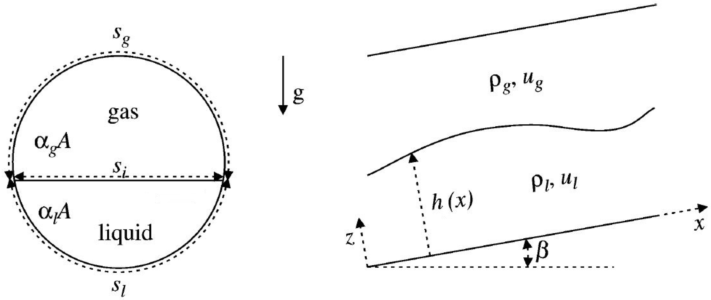
Figure 2.
The algorithm implemented to obtain the values of and .

Figure 3.
Plot of the amplification factor for different couples of inlet superficial velocities. (a) Amplification factor for geometry Pipe1; and (b) amplification factor for geometry Pipe2.
Figure 3.
Plot of the amplification factor for different couples of inlet superficial velocities. (a) Amplification factor for geometry Pipe1; and (b) amplification factor for geometry Pipe2.

Figure 4.
Flow pattern maps. Points stand for the simulation results; ×: smooth stratified flow, ▽: wavy stratified flow, ∘: slug flow. Comparison against the theoretical Viscous Kelvin–Helmholtz (VKH) line and the Inviscid Kelvin–Helmholtz (IKH) line. (a) Pipe1 flow pattern map; and (b) Pipe2 flow pattern map.
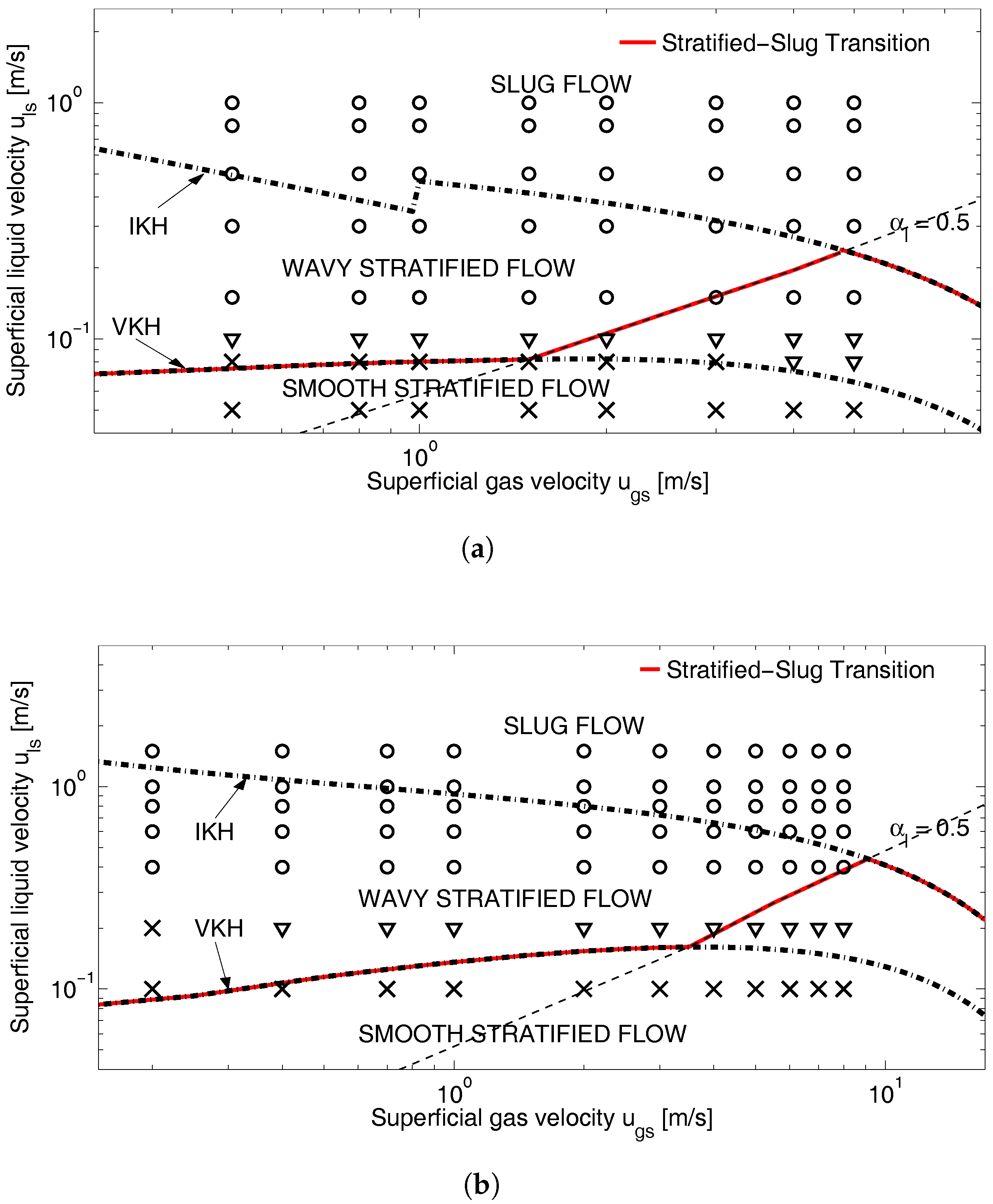
Figure 5.
Slug mean velocity: numerical results are bounded by the confidence lines. (a) Pipe1: numerical results against experimental data (left) and comparison with the relation by [47] (right); and (b) Pipe2: numerical results against empirical correlation.
Figure 5.
Slug mean velocity: numerical results are bounded by the confidence lines. (a) Pipe1: numerical results against experimental data (left) and comparison with the relation by [47] (right); and (b) Pipe2: numerical results against empirical correlation.
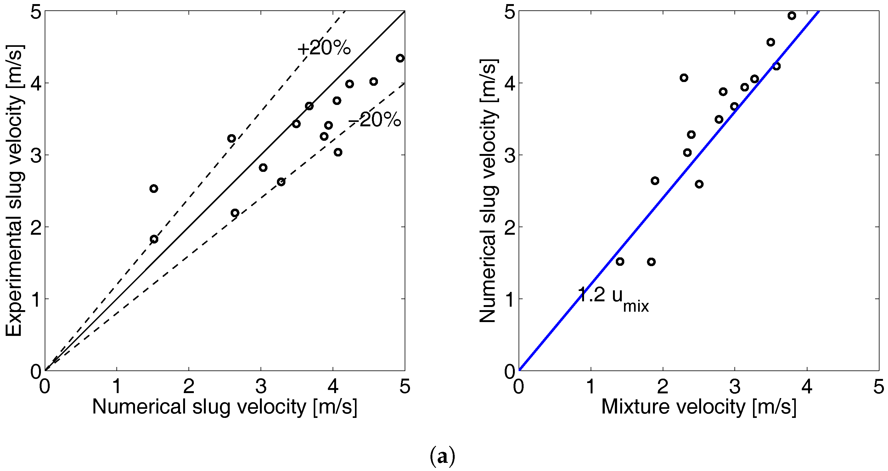
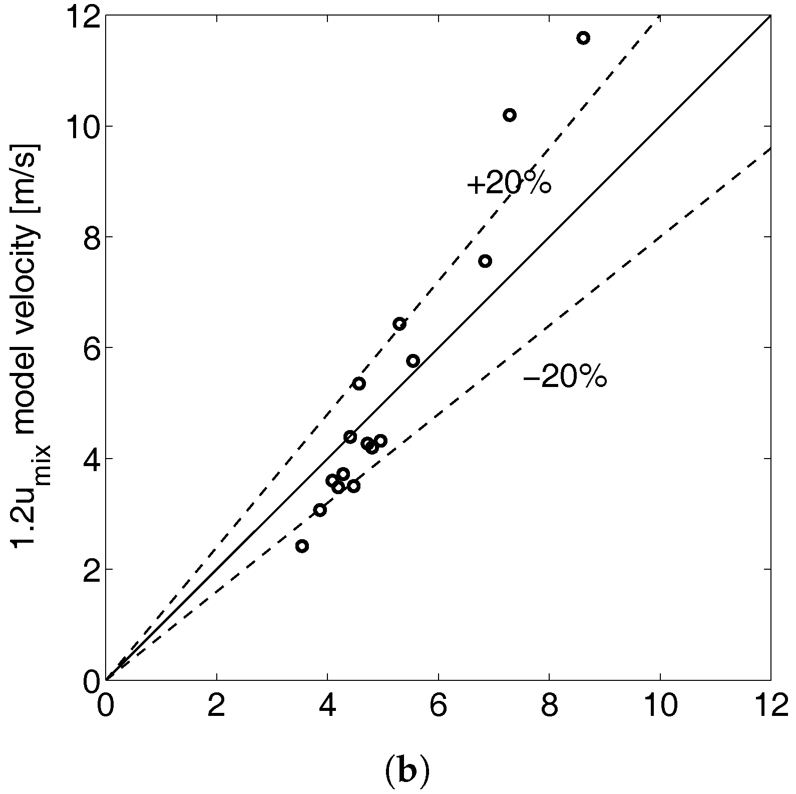
Figure 6.
Slug mean frequency: several numerical results are bounded by the confidence lines. (a) Pipe1: numerical results against experimental data; and (b) Pipe2: numerical results against empirical correlation.
Figure 6.
Slug mean frequency: several numerical results are bounded by the confidence lines. (a) Pipe1: numerical results against experimental data; and (b) Pipe2: numerical results against empirical correlation.

Figure 7.
Typical slug length distribution for the presented geometries. (a) Pipe1. Left: = 1.1 m/s and = 1.3 m/s. Right: = 1.5 m/s and = 1.6 m/s; and (b) Pipe2. Left: = 2.0 m/s and = 1.0 m/s. Right: = 2.5 m/s and = 1.0 m/s.
Figure 7.
Typical slug length distribution for the presented geometries. (a) Pipe1. Left: = 1.1 m/s and = 1.3 m/s. Right: = 1.5 m/s and = 1.6 m/s; and (b) Pipe2. Left: = 2.0 m/s and = 1.0 m/s. Right: = 2.5 m/s and = 1.0 m/s.
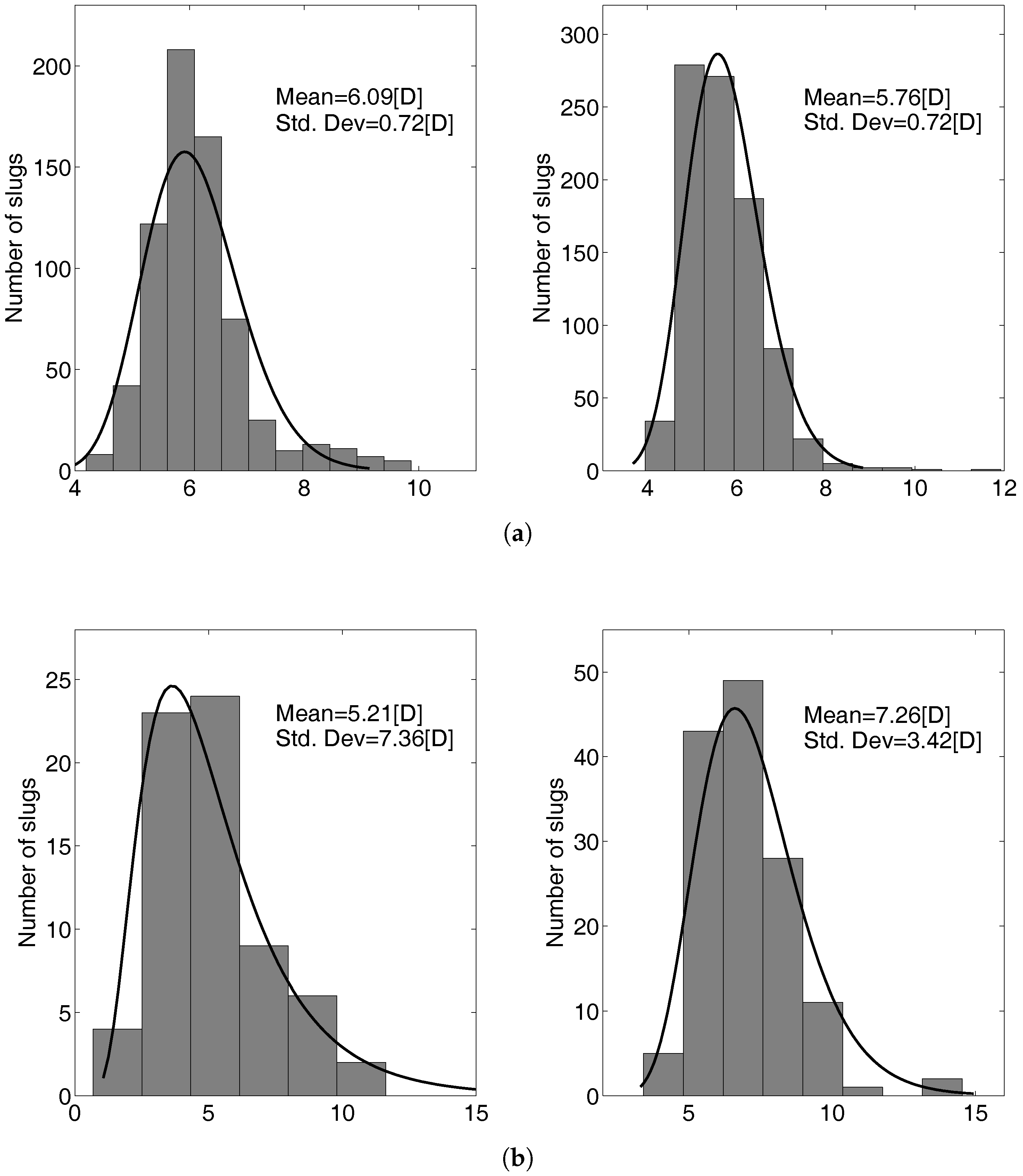
Figure 8.
Dimensionless computational time as a function of the superficial gas velocity: simulations with the lower superficial velocities are performed faster than real time. End time t = 300 s, x = , . (a) Dimensionless computational time for the simulations performed on Pipe1; and (b) Dimensionless computational time for the simulations performed on Pipe2.


Table 1.
Geometrical characteristics, mesh sizes and superficial velocity ranges of the pipes analyzed in the numerical results.
Table 1.
Geometrical characteristics, mesh sizes and superficial velocity ranges of the pipes analyzed in the numerical results.
| Geometry | Length (m) | Diameter (m) | (m/s) | (m/s) |
|---|---|---|---|---|
| Pipe1 | 9 | 0.5–5.0 | 0.05–1.6 | |
| Pipe2 | 36 | 0.2–10.0 | 0.1–2.5 |
Table 2.
Physical properties of the adopted fluids.
| Fluid | (kg/m3) | (Pa · s) |
|---|---|---|
| air (g) | ||
| water (l) | 1000 |
© 2017 by the authors. Licensee MDPI, Basel, Switzerland. This article is an open access article distributed under the terms and conditions of the Creative Commons Attribution (CC BY) license (http://creativecommons.org/licenses/by/4.0/).
Share and Cite
MDPI and ACS Style
Bonzanini, A.; Picchi, D.; Poesio, P. Simplified 1D Incompressible Two-Fluid Model with Artificial Diffusion for Slug Flow Capturing in Horizontal and Nearly Horizontal Pipes. Energies 2017, 10, 1372. https://doi.org/10.3390/en10091372
AMA Style
Bonzanini A, Picchi D, Poesio P. Simplified 1D Incompressible Two-Fluid Model with Artificial Diffusion for Slug Flow Capturing in Horizontal and Nearly Horizontal Pipes. Energies. 2017; 10(9):1372. https://doi.org/10.3390/en10091372
Chicago/Turabian StyleBonzanini, Arianna, Davide Picchi, and Pietro Poesio. 2017. "Simplified 1D Incompressible Two-Fluid Model with Artificial Diffusion for Slug Flow Capturing in Horizontal and Nearly Horizontal Pipes" Energies 10, no. 9: 1372. https://doi.org/10.3390/en10091372
Note that from the first issue of 2016, this journal uses article numbers instead of page numbers. See further details here.