Multi-Objective Optimization of the Hydrodynamic Performance of the Second Stage of a Multi-Phase Pump

Abstract

Most multi-phase pumps used in crude oil production have been developed to satisfy certain pressure specifications. In the design of these pumps, the flow characteristics of the posterior stage are different from those of the prior stage. For this reason, the design of the second stage needs to be supplemented. To optimize performance in this stage, multi-objective optimization to simultaneously increase pressure and efficiency is reported in this article. Flow analyses of the single and multiple phases of the multi-phase pump were conducted by solving three-dimensional steady Reynolds-averaged Navier–Stokes equations. For the numerical optimization, two design variables related to the blade inlet angle were selected. The impeller and the diffuser blades were optimized using a systematic optimization technique combined with a central composite method and a hybrid multi-objective evolutionary algorithm coupled with a surrogate model. The selected optimal model yielded better hydrodynamic performance than the base model, and reasons for this are investigated through internal flow field analysis.

1. Introduction

Multi-phase pumps constitute core machinery in the offshore plant industry. They are installed in oil wells to pressurize and transport crude oil. As some recent oil wells are located in deep waters, the pressure specifications for the pumps used have been increased. Therefore, most multi-phase pumps used in such oil wells have been designed to function in multiple stages to satisfy these pressure specifications [1,2].

In the design of multistage pumps, the flow characteristics of the posterior stage are different from those of the prior stage. Hence, inflow characteristics need to be considered according to stage while designing multistage pumps.

Many studies have been conducted to maximize the performance of each stage. The inverse design method was coupled with the computational fluid dynamics (CFD) and an optimizer for single-objective numerical optimization [3,4]. Multi-point or multi-objective optimization has also been proposed to design experiments combined with multi-objective evolutionary algorithms [5,6]. The trend toward multi-disciplinary approaches has led to the consideration of more design variables and objective functions for such pumps.

The authors of this article have systematically studied multi-phase pumps in past work [7,8,9,10,11]. Here, to maximize the performance of multi-phase pumps, multi-objective optimization to simultaneously improve their pressure and efficiency is proposed and tested. The second stage in multi-phase pumps is chosen as the subject of study because differences in flow characteristics are remarkable between a single-stage pump and the second stage of a multi-phase pump. When designing multistage pumps, this discordance in flow and blade angles needs to be considered. The second stage of the impeller and the diffuser blades is optimized using a systematic optimization technique combined with a central composite method and a hybrid multi-objective evolutionary algorithm coupled with a surrogate model. The causes of the performance improved compared with the base model are then analyzed through comparisons of their internal flow fields.

2. Multi-Phase Pump Model

In the organization of turbomachinery, Cordier created a diagram grouped into different regions, such as centrifugal flow, mixed flow, and axial flow on a speed-specific diameter [12]. Axial flow pumps and inducers can be classified into ranges of roughly 3 < Ns < 6 and 1.25 < Ds < 1.65.

Helico-axial multi-phase pumps are composed of a rotating part (the impeller) and a stationary part (the diffuser) as shown in Figure 1. The design of impellers, the profiles of which are derived from the NACA 65 series airfoil, can be used to avoid the phase separation of gas and liquid, yielding good performance in terms of conveying multi-phase flow. The shape of the blade resembles that of an inducer with very low blade height. Downstream of the impeller, the diffuser not only recovers the hydraulic pressure but also guides the fluid flow direction at the diffuser outlet for the next stage impeller.

The impeller and diffuser from the first stage, optimized through an examination of past studies, were selected as the base model of the second stage in this study [10]. The design flow rate, static pressure rise, and the rotational speed of the helico-axial pump were 110 m³/h, 360 kPa, and 3600 r/min, respectively. With these operating conditions, the flow coefficient (φ) and the work coefficient (ψ) were 0.061 and 0.501, respectively. The detailed design information is shown in

Table 1. Design information of second-stage base model.

Variables	Impeller	Diffuser
Number of blades (EA)	3	11
Tip clearance (mm)	0.5	None
Width of the inlet (mm)	22.5	14.5
Width of the outlet (mm)	14.5	22.5
Inlet blade angle at hub (°)	11.3	18.5
Inlet blade angle at shroud (°)	8	18
Outlet blade angle at hub (°)	30	90
Outlet blade angle at shroud (°)	25	90

. The base impeller of the second stage was composed of three blades each with a diameter of 150 mm. The blades’ inlet and outlet angles were 11° and 25°, respectively, and formed the basis of the shroud. The space between the first-stage diffuser and the second-stage impeller was set to 16.5 mm, identical to the space between the impeller and the diffuser in the first stage.

3. Numerical Method

3.1. Single-Phase Flow Scheme

The performance of the second stage of the multi-phase pump was evaluated using numerical simulations. Experiments were conducted to verify the reliability of the numerical analysis [7,8,9,10,11]. Figure 2 shows the domain of the numerical analysis and the schemes used for performance evaluation. To reduce time consumed and the cost of analysis, periodic conditions were imposed to select the blade one-passage domain. A grid system was formed with structured meshes using ANSYS TurboGrid version 16.1, and the impeller domain was composed of approximately 430,000 nodes whereas the diffuser was composed of approximately 300,000 nodes. Moreover, considering the applied turbulence model, the y+ value of the grids close to the wall was set to 2 or smaller.

A computational fluid dynamics (CFD) simulation was conducted using ANSYS CFX, a commercial viscous fluid analysis program. The three-dimensional (3D) Reynolds-averaged Navier–Stokes (RANS) equation was used for turbulent flow analysis to examine the characteristics of flow fields inside the multi-phase pump, and the governing equation used was discretized with the finite volume method (FVM). A high-resolution scheme with at least second-order accuracy was used as the discretizing scheme. A shear stress transport model suitable for the prediction of flow separations was used as the turbulence model for the analysis of turbulent flows [13].

Atmospheric pressure conditions were imposed on the inlet and flow-rate conditions on the outlet as boundary conditions for the numerical analysis, and the stage average condition was imposed as an interface condition between domains. Water at 25 °C was selected as the working fluid.

3.2. Multi-Phase Flow Scheme

When simulating multi-phase flows, a number of physical phenomena are important, such as buoyancy, interphase drag or exchange of momentum, surface tension, turbulence effects, and dispersed phase particle–particle interactions. For gas–liquid flows, the density of the different phases can differ by a factor of 1000, and hence the effects of buoyancy must be taken into account. At low-volume fractions (usually GVF ≤ 5%) of the dispersed phase, the probability of interaction between dilute dispersed phases is much smaller than that of interactions in the continuous phase [14,15]. Under these conditions, particle–particle interactions may be neglected, and single-particle/droplet/bubble correlations or theory may be applied. As the volume fraction increases, particle–particle interactions become significant and dilute system approximations may no longer be valid.

The multiphase flow models were used in the three-dimensional viscous fluid analysis program ANSYS CFX ver. 17.1 [16]. The Eulerian–Eulerian two-fluid approach is typically used to analyze the internal multi-phase flow of the helico-axial pump [17]. The two-fluid approach can be divided into homogenous and inhomogeneous types depending on the approach. Multiphase pump in an air-water flow is predominated by centrifugal force. Due to the density differences, the dispersed phase accelerates relative to the continuous phase. The inhomogeneous fluid approach shares only the pressure field for each phase and performs separate analyses for other variables. Moreover, the particle model performs analysis under the assumption that the particles of each phase are maintained independently. The multi-phase flow is simulated as isothermal, without heat and mass transfer between the continuous and the dispersed phases, so that the equations of continuity and momentum for the phases can be discretized to solve for the unknown parameters. The laws of conservation of inhomogeneous momentum can be expressed as follows:

$$\begin{array}{l}\frac{\partial }{\partial t}(r_c{\rho }_c{U}_c)+\nabla (r_c{\rho }_c{U}_c{U}_c)=-r_c\nabla P_c+\nabla (r_c{\mu }_c(\nabla U_c+{[U_c]}^T))\\ +{\displaystyle \sum _{d=1}^{{{\displaystyle N}}_p}}({\mathrm{\Gamma }}_{cd}{U}_d-{\mathrm{\Gamma }}_{dc}{U}_c)+{\displaystyle \sum _{d=1}^{{{\displaystyle N}}_p}}{F}_{inter.cd}\end{array}$$

(1)

In the above equation, r_c, ρ_c, μ_c, U_c, and U_d are the volume fraction, the density of the continuous phase, the viscosity of the continuous phase, and the velocity of the continuous and the disperse phases, respectively. t represents the simulation time, and F_inter.cd denotes the total interfacial forces applied to the continuous and the dispersed phases:

$$F_{inter.cd}=F_{drag}+F_{lift}+F_{w.l}+F_{v.m.}+F_{t.d.}$$

(2)

F_inter.cd is the sum of drag, lift, wall lubrication, virtual mass, and the turbulence dispersion force. Each interphase model was highly reliable.

The important physical phenomena in the use of the interphase force models and the bubble diameter were summarized according to GVF as shown in

Table 2. The interphase force models and bubble diameter.

Interphase Transfer	Particle Model
Drag force	Grace model [18]
Lift force	Tomiyama model [19]
Wall lubrication force	Antal model [20]
Turbulence dispersion force	Lopez de Bertodano [21]
Turbulence transfer	Sato Enhanced Eddy Viscosity [22]
Gas volume fraction (%)	5	10	15
Initial bubble diameter (mm)	0.4	0.7	1.0

. Each interphase model was applied such that the air-water bubbly flow was well simulated with high reliability. The fluid between two adjacent impellers and diffusers was assumed to be a periodic condition in the direction of rotation. Boundary conditions, velocity and gas volume fractions using the CFX Expression Language (CEL) conditions were set as inlet conditions, and atmospheric pressure conditions were set as the outlet condition. A stage average was applied as an interface condition between the rotating and the stationary domains. This model enabled steady-state predictions to be obtained for multi-stage machines. Stage analysis is most appropriate when the circumferential variation in flow is of the order of the component pitch. The interfaces between other domains were set using the frozen rotor method.

4. Multi-Objective Optimization

The multi-objective optimization problem is in general defined to optimize each objective function under a group of constraints. For example, when an objective function is improved, another objective function is decreased, and vice versa. Therefore, it is challenging to devise a solution that simultaneously improves multiple objective functions. The solution to a multi-objective problem is one where designers select solutions from Pareto-optimal frontiers or non-dominant solutions as the optimum ones. The overall multi-objective optimization procedure is shown in Figure 3.

The purpose of this optimization is to maximize the hydraulic performance of a multi-phase pump in terms of efficiency and pressure rise, which are defined as follows:

$${\eta }_p=\frac{\rho mgHQ}{T\omega }$$

(3)

$$∆\mathrm{P}=P_{oulet}-P_{inlet}$$

(4)

$${\alpha }_c+{\alpha }_d=1$$

(5)

$${\rho }_m={\alpha }_c{\rho }_c+{\alpha }_d{\rho }_d$$

(6)

where ${\alpha }_c$, ${\alpha }_d$, ${\rho }_m$, ${\rho }_d$, g, H, Q, T, ω, ΔP, $P_{oulet}$ and $P_{inlet}$ represent gas volume fraction of continuous and dispersed phase, mixture density, density of dispersed phase, acceleration of gravity, head, volume flow rate, blade torque, angular velocity, pressure rise, pressure rise at the outlet, and pressure rise at the inlet, respectively.

Differences in flow characteristics are evident in the impeller in the second stage because of the secondary flow in the passage of a single-stage diffuser. Due to discordance between flow and the blade angles, the hub inlet angle (I_beta1_hub) and the shroud inlet angle (I_beta1_shr) were selected as design variables of the second impeller. Moreover, the wrap angle was selected as the constraint to fix the value for this study. In general, the wrap angle is related to the determination of the outlet angles, so the specific angle was determined to obtain the best efficiency point at the design flow rate in light of target pressure performance using data accumulated from the single-objective optimization of the single- and second-stage impellers and diffusers [23]. The beta angle and the theta angle of the blade have a trigonometric relationship. If we know the meridional length and the theta angle, we can determine the beta angle [24]. Moreover, when the blade’s inlet angles and the wrap angles are known, its outlet angles can be automatically determined. The impeller’s hub outlet angle (I_beta2_hub) and the shroud outlet angle (I_beta2_shr) were not selected as independent but as dependent variables in this study. In other words, the design variables of the impeller were selected to control both the inlet and the outlet angles in accordance with the constraints shown in Figure 4.

The selected design variables for the diffuser’s hub inlet angle (D_beta1_hub) and the shroud’s inlet angle (D_beta1_shr) are shown in Figure 5. The outlet angle of the diffuser was designed to decelerate flow and deflect it along an axis direction that increased the static pressure of the fluid. Therefore, the diffuser’s hub and the shroud’s outlet angles (D_beta2_hub, D_beta2_shr) were fixed at 90°.

For design optimization, it is important to find a feasible design space formed by ranges of the design variables. The ranges of the changes were selected based on the flow angle at the leading and the trailing edges along the span of the base impeller of the second stage. Nine training points within the design space were generated with the help of central composite design (CCD) [25,26]. The selected feasible design ranges and training points are listed in

Table 3. Feasible design ranges and training points.

(a) Impeller
Variables	Lower Bound	Center		Upper bound
I_beta1hub (°)	7	11		15
I_beta1shr (°)	7	11		15
Set	Independent Variables		Dependent Variables
	I_beta1hub (°)	I_beta1shr (°)	I_beta2hub (°)	I_beta2shr (°)
1	11	11	36	22.5
2	11	7	36	31
3	8	8	43	28
4	14	14	30	18.5
5	7	11	48	22.5
6	11	15	36	17.5
7	15	11	28	22.5
8	14	8	30	28
9	8	14	43	18.5
(b) Diffuser
Variables	Lower Bound	Center		Upper bound
D_beta1hub (°)	18	22		26
D_beta1shr (°)	18	22		26
Set	Independent Variables		Fixed Variables
	D_beta1hub (°)	D_beta1shr (°)	D_beta2hub (°)	D_beta2shr (°)
1	22	22	90	90
2	22	18
3	25	25
4	25	19
5	18	22
6	19	19
7	19	25
8	22	26
9	26	22

, and all portions of the design space are represented in Figure 6. The objective functions at these design points were calculated by 3D RANS analysis.

Multi-objective optimization based on evolutionary algorithms combined with a surrogate model requires many calculations of the objective functions in the search for optimal solutions. The response surface approximation (RSA) [27,28] model was employed as the surrogate model and was used to predict the objective function values in the design space. The RSA model was constructed to approximate the objective function values for an evolutionary algorithm, and a hybrid multi-objective evolutionary algorithm (MOEA) was used to obtain global Pareto-optimal solutions (POSs). Approximate POSs were obtained using the real-coded, fast, and elitist non-dominant sorting genetic algorithm (NSGA-II) developed by Deb [29] for two objective functions, the total efficiency and the total pressure. Here, “real-coded” indicates that crossovers and mutations were performed in real space to obtain a response from the NSGA-II. The POSs were refined by searching for a local optimal solution for each objective function over all the NSGA-II-derived optimal solutions, where the search used sequential quadratic programming (SQP) [30] with NSGA-II solutions as initial guesses.

5. Results and Discussion

Results of Multi-Objective Optimization

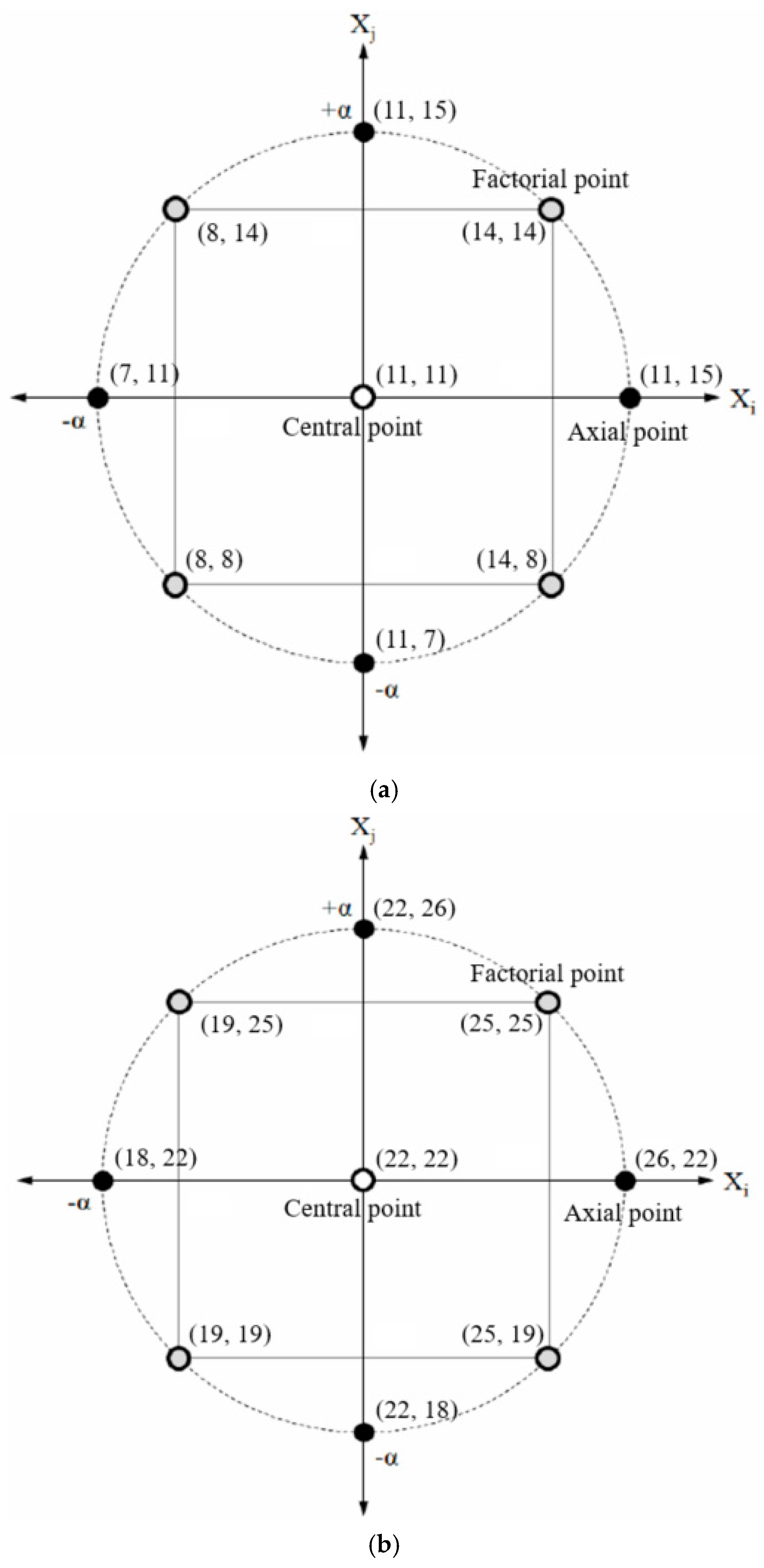
The multi-objective optimizations of the second impeller and the second diffuser were performed sequentially. Based on the results of a numerical analysis of the test sets generated through CCD, regression analyses of the RSA surrogate model were conducted and multi-objective optimization was performed to obtain the global POSs, as shown in Figure 7. The results of the regression analysis of the response surface, including the root mean-square error (RMSE) of the multi-objective function, were analyzed by the RSA. For acceptable accuracy, the value of R_adj² needed to be in the range 0.9 < R_adj² < 1.0 [31]. The values of R_adj² for total efficiency and total pressure were 0.9912 and 0.9885, respectively. Thus, all predicted values obtained using the RSA models were reliable. The functional forms from the RSA model can be expressed in terms of design variables normalized as follows:

$${\mathsf{\Delta }\mathrm{P}}_{total}= 474.478-3.6714x_1+19.1013x_2-23.8548x_1{x}_2-4.2537x_1^2-22.9908x_2^2$$

(7)

$${\eta }_{total}= 66.2156-2.2609x_1+4.9018x_2-1.5999x_1{x}_2-1.3983x_1^2-3.2375x_2^2$$

(8)

where $x_1$ and $x_2$ represent the impeller’s hub inlet angle (I_beta1_hub) and the shroud’s inlet angle (I_beta1_shr), respectively.

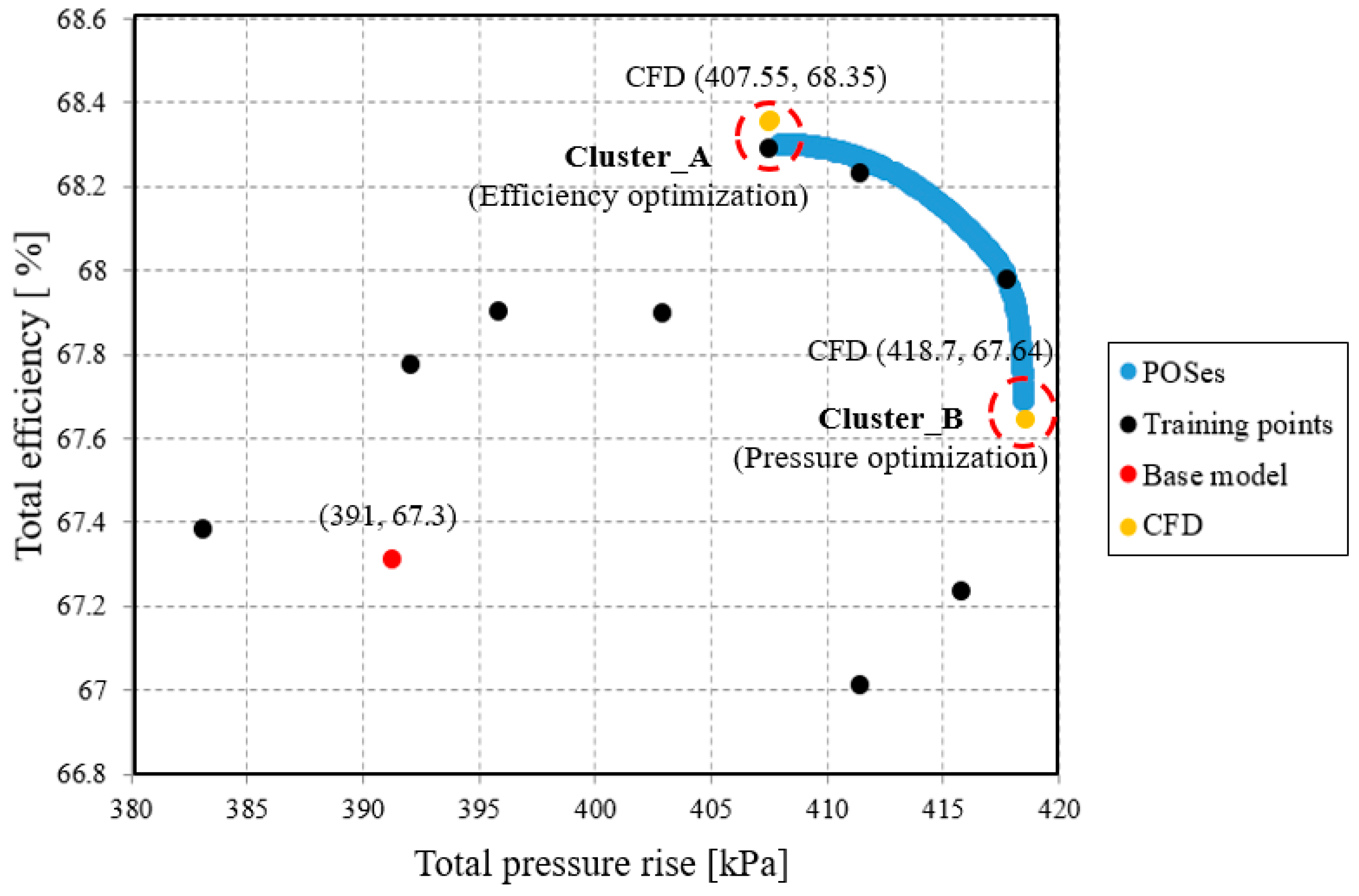
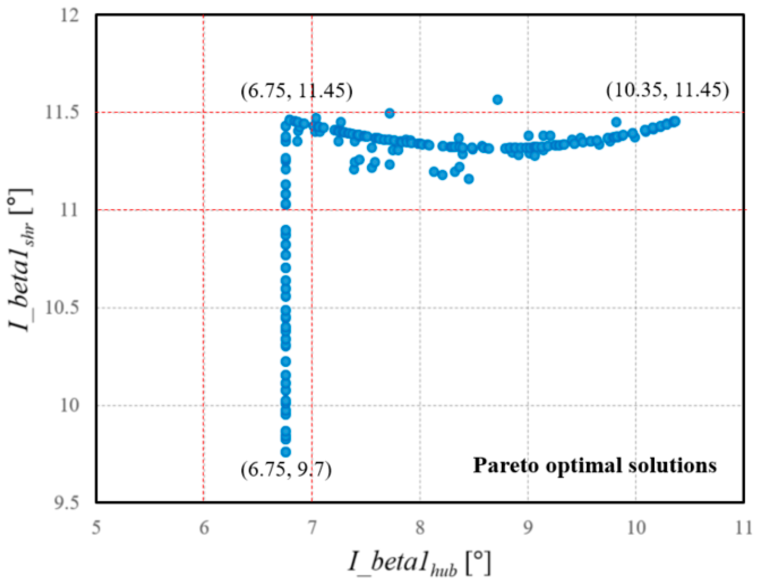
A trade-off analysis shows an obvious correlation between total efficiency and total pressure. In other words, the improvement in total efficiency led to a deterioration in total pressure performance, and vice versa. Designers will use one or several solutions from POSs as the optimum solution(s) to solve multi-objective optimization problems. Cluster_A shows an efficiency optimization model and Cluster_B a pressure optimization model. Two arbitrarily clustered optimum models, oriented for each objective function, were selected in the POSs and calculated through CFD analysis. Their results are in agreement with the predicted values generated by the POSs, and both points presented visibly increased hydraulic performance compared with the base model. Cluster_A showed an increase of 1.1% in total efficiency and that of 16.3 kPa in total pressure, and Cluster_B showed an increase of 0.34% in total efficiency and 27.7 kPa in total pressure. Cluster_A, which was near the end of the global POSs, was selected as the final model of the second-stage impeller. Since the impeller and the diffuser in the first stage had been optimized to improve hydraulic efficiency, this study focused on efficiency-oriented design to maximize stage performance [10]. The results of the multi-objective optimization of the second impeller are shown in

Table 4. Results of the multi-objective optimization for the 2nd impeller.

	Base Model	Optimum Model
Inlet blade angle hub (β1h) (°)	11	10.5 (−0.5)
Inlet blade angle shr (β1s) (°)	8	11.5 (+3.5)
Outlet blade angle hub (β2h) (°)	30	34 (+4)
Outlet blade angle shr (β2s) (°)	25	22.5 (+2.5)
Total pressure rise (kPa)	391	407.55 (+16)
Total efficiency (%)	67.3	68.35 (+1.05)
Pareto-optimal solution (kPa/%)	-	407.51/68.58
CFD prediction (kPa/%)	-	407.55/68.35
Error (kPa/%)	-	+0.04/−0.23

.

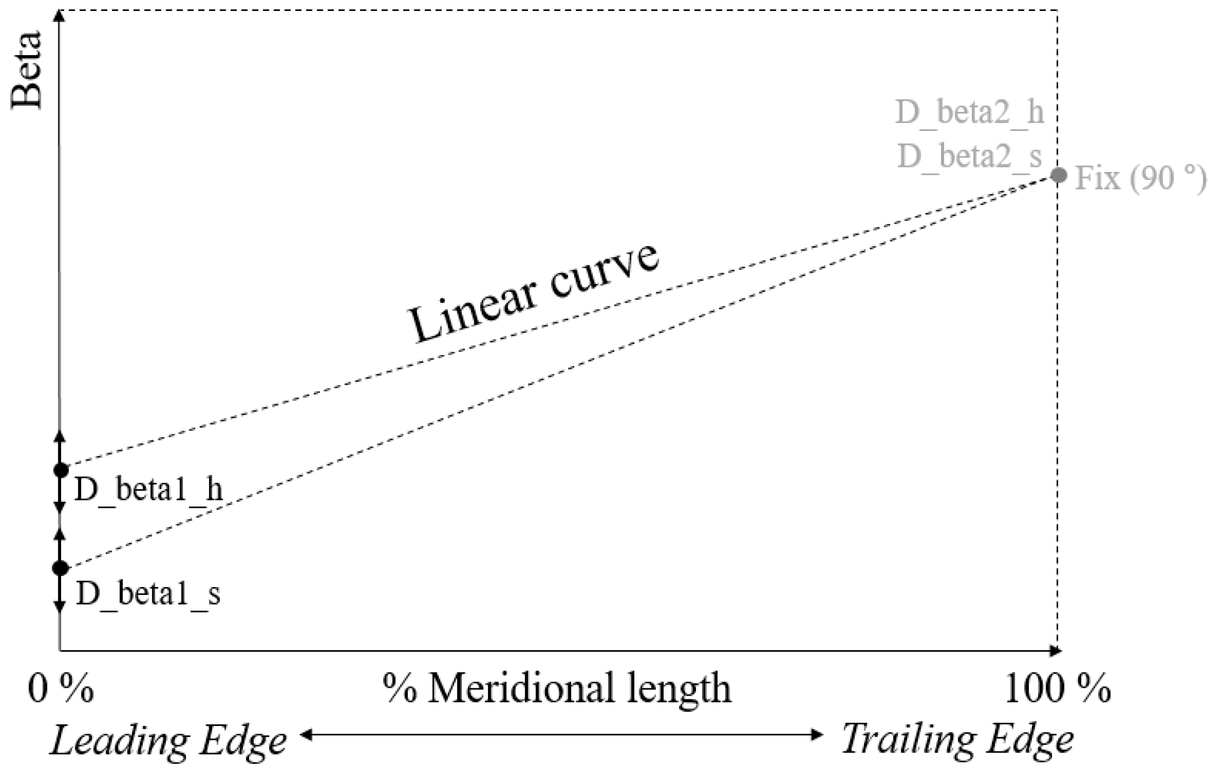
The independent design variables of the inlet blade angle at the hub were reduced by 0.5 degrees, and the inlet blade angle at the shroud increased by 3.5 degrees. This indicates that the impeller’s shroud angle at the inlet (I_beta1_shr) was much more sensitive than the diffuser’s hub angle at the inlet (I_beta1_hub). Moreover, the dependent design variables of the outlet blade angle at the hub and the shroud increased by 4.0 degrees and 2.5 degrees, respectively.

Figure 8 shows the optimal angle distribution of the second-stage impeller. When the inlet blade angle at the hub increased, the performance oriented the pressure optimization. On the other hand, when the inlet blade angle at the shroud increased, the performance oriented the pressure optimization. In accordance with the constraints, in case of the inlet and the outlet angles, the tendency was inversely proportional. For example, as the inlet blade angle at the hub increased, efficiency increased and pressure decreased. The outlet hub angle, on the contrary, showed a tendency whereby efficiency decreased and pressure increased.

Results for the analysis of the response surface of multi-objective optimization to find the optimal point for the hydraulic performance of the diffuser are shown in Figure 9. The values of R² and R²_adj, the explanatory power of the regression model, were 0.9863 and 0.9765, respectively. For the multi-objective optimization of the second diffuser, the multiple linear regression equation can be expressed for static efficiency and pressure as follows:

$${\mathsf{\Delta }\mathrm{P}}_{static}= 239.9+4.96x_1+7.18x_2-0.1531x_1{x}_2-0.0509x_1^2-0.0717x_2^2$$

(9)

$${\eta }_{static}= 37.52+1.081x_1+1.182x_2-0.02667x_1{x}_2-0.01345x_1^2-0.01135x_2^2$$

(10)

where $x_1$ and $x_2$ represent the diffuser’s hub inlet angle (D_beta1_hub) and the shroud’s inlet angle (D_beta1_shr), respectively.

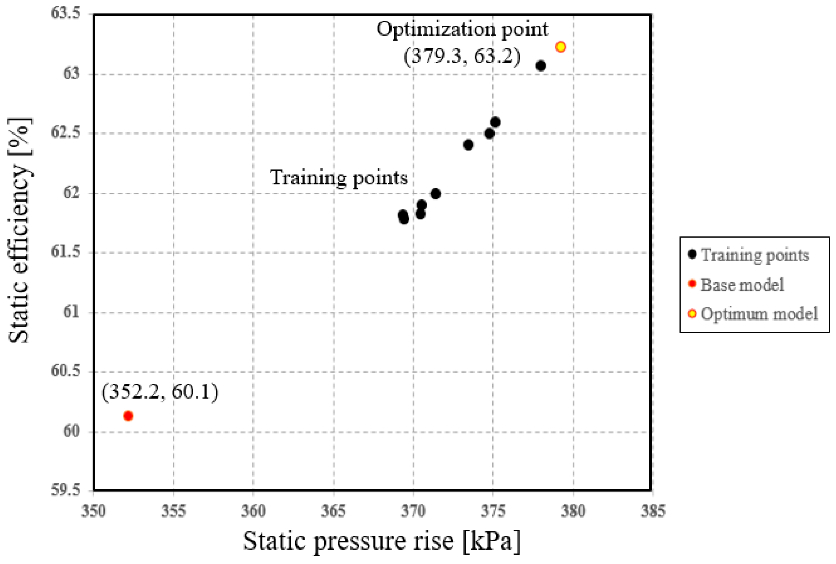
In the case of the diffuser, there was no trade-off characteristic due to an obvious correlation between static efficiency and static pressure. The predicted performance in terms of static pressure and efficiency were 379.61 kPa and 63.25%, respectively, using the surrogate model and sequential quadratic programming. They were calculated at 379.3 kPa and 63.22%, respectively. The static efficiency of the optimum diffuser hence increased by 3.1% and the static pressure by 27 kPa compared with the base model in single-phase flow. The results of the multi-objective optimization of the second diffuser are shown in

Table 5. Results of the multi-objective optimization for the 2nd diffuser.

	Base Model	Optimum Model
Inlet blade angle hub (β1h) (°)	18.5	18 (−0.5)
Inlet blade angle shr (β1s) (°)	18	26 (+8)
Outlet blade angle hub (β2h) (°)	90	90 (fixed)
Outlet blade angle shr (β2s) (°)	90	90 (fixed)
Static pressure rise (kPa)	352.2	379.3 (+27.1)
Static efficiency (%)	60.12	63.22 (+3.1)
RSA optimal (kPa/%)	-	379.61/63.25
CFD prediction (kPa/%)	-	379.3/63.22
Error (kPa/%)	-	+0.31/0.03

. Independent design variables of the inlet blade angle at the hub decreased by 0.5 degrees, and the inlet blade angle at the shroud increased by 8.0 degrees. Both the inlet angles at the hub and the shroud showed a similar sensitivity to the objective function.

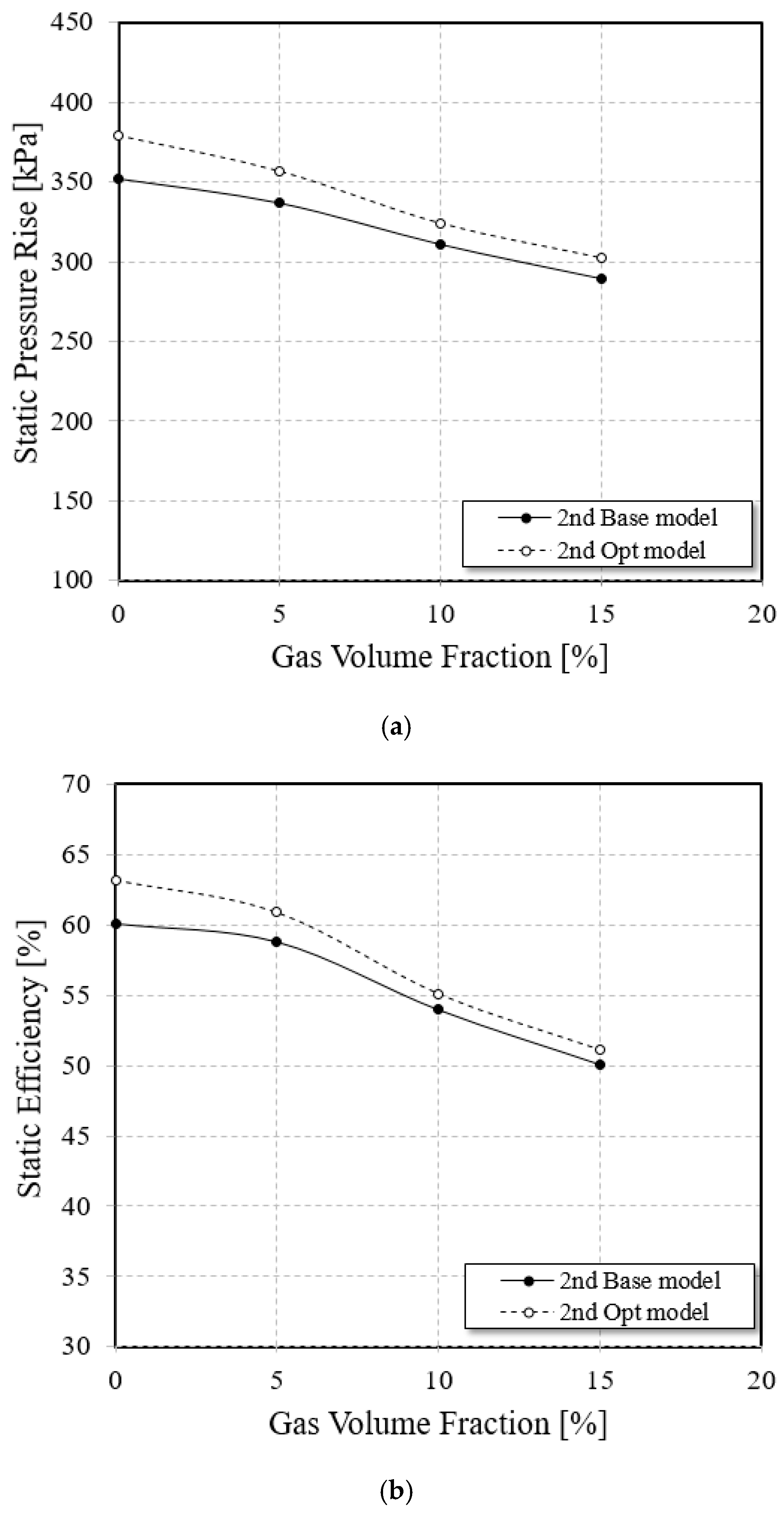
A comparison of hydraulic performance between the base and the optimum models in terms of the design flow rate was calculated along the GVF ranges as shown in Figure 10. As the increase in the size and number of bubbles caused them to be more closely spaced, it affected the internal pressure with increasing GVF. When the GVF was 0%, 5%, 10%, and 15%, the static efficiencies of the optimum model were 63.22%, 60.91%, 55.09%, and 51.10%, respectively, and the static pressure increases of the optimum model were calculated as 379.3 kPa, 357 kPa, 324 kPa, and 302 kPa, respectively.

The increase in static pressure and the static efficiency of the optimum model generally increased along the GVF, up to 15% compared with the base model, as shown in

Table 6. The optimum model increased performance compared to the base model.

Designs	GVF 0 [%]		GVF 5 [%]		GVF 10 [%]		GVF 15 [%]
	ΔPstatic [kPa]	ηstatic [%]	ΔPstatic [kPa]	ηstatic [%]	ΔPstatic [kPa]	ηstatic [%]	ΔPstatic [kPa]	ηstatic [%]
Base model	352.2	60.12	337	58.82	311	53.99	289	50.10
Opt model	379.3	63.22	357	60.91	324	55.09	302	51.10
Relative Improvement (comparison to base)	+27.1	+3.1	+20	+2.1	+13	+1.1	+13	+1

.

To determine the main factors influencing the improvement in performance, internal flow fields for single- and multi-phase flows were examined as shown in Figure 11, Figure 12, Figure 13, Figure 14 and Figure 15.

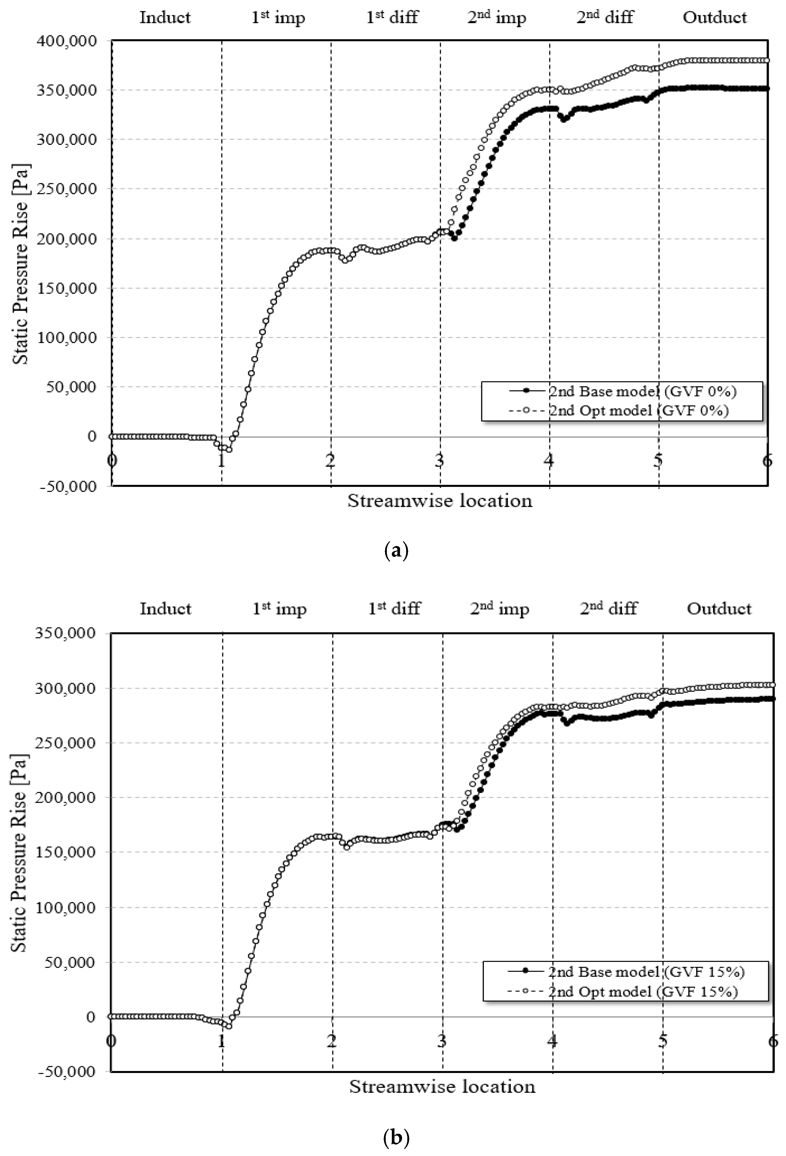
Distributions of static pressure at 50% that span along the streamwise location are shown in Figure 11. These results indicated that the overall static pressure distribution of the optimum model generally improved compared with that of the base model from the inlet to the outlet. It was confirmed that a higher pressure increase was achieved in the second impeller. Downstream of the impeller, deceleration in flow movement and pressure recovery were observed in the second diffuser.

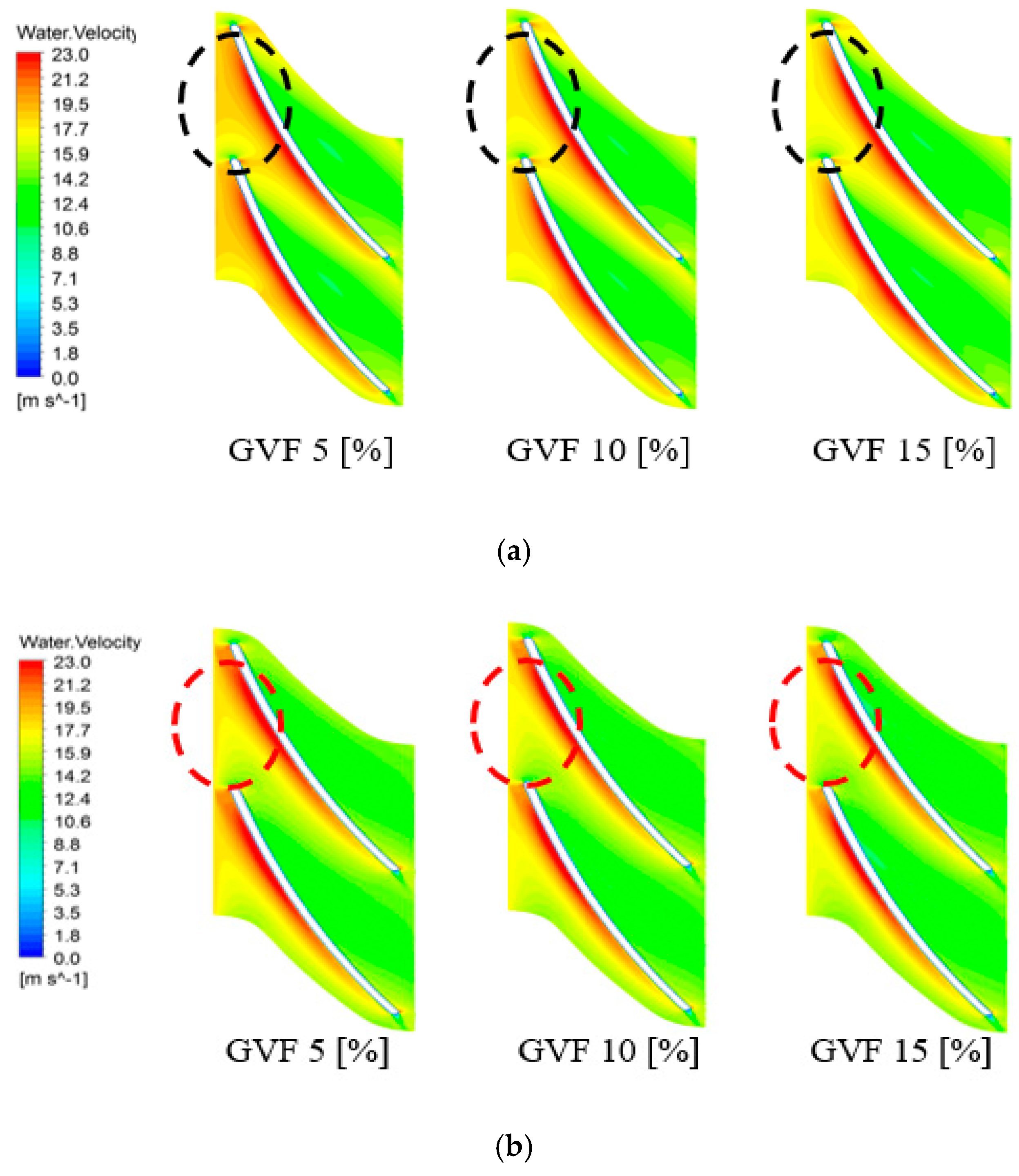
Figure 12 shows the instantaneous velocity contour mid-span with increasing GVF. In the base model, a region of non-uniform flow was remarkable at the impeller’s leading edge because of the discrepancy between flow angle and blade angle. Due to the positive incidence angle on the surface around the impeller, the detached flow was predominant on the suction surface. The unstable fluid flow induced a negative effect on the performance of pressure rise. On the other hand, in the case of the optimum model, these non-uniform flow components were suppressed and the velocity contour was uniform in comparison with the base model.

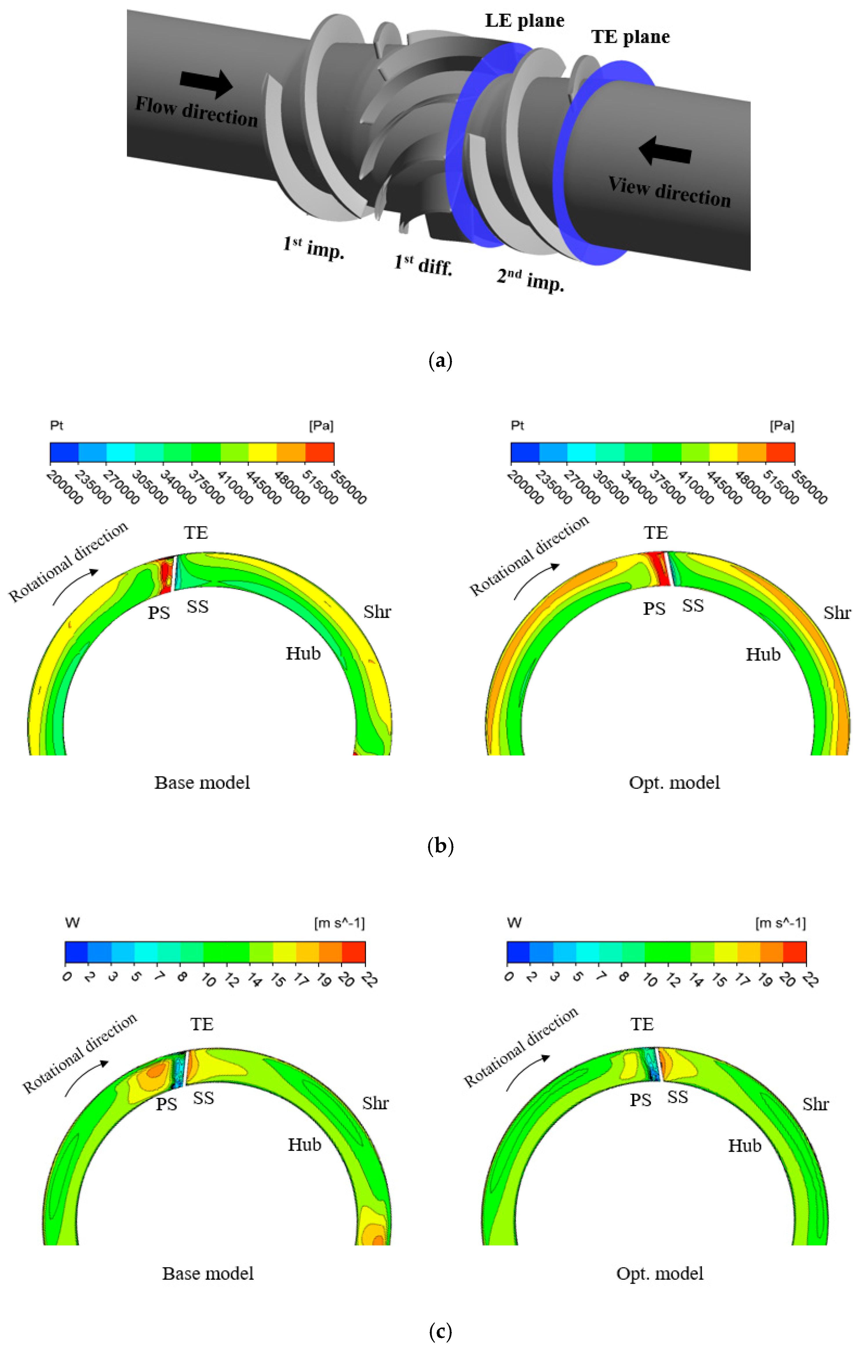
Figure 13 shows internal flow contours near the trailing edge of the second impeller. The location of observation is shown in Figure 13a. As shown in Figure 13b, the optimum model at the impeller outlet showed a high level of increase in relative total pressure. However, non-uniform flow field components existed from the hub to the shroud in the base model. According to the flow stabilization of the upstream region, the total pressure distributions were generally uniform in the optimum impeller. Furthermore, the deviation in flow at the trailing edge was due to the effects of blade loading, which created a pressure difference between the pressure and the suction sides. These non-uniform flow components were suppressed in the optimum model, and internal flow distributions along the spanwise direction were generally uniform—especially near the region of pressure side—as shown in Figure 13c.

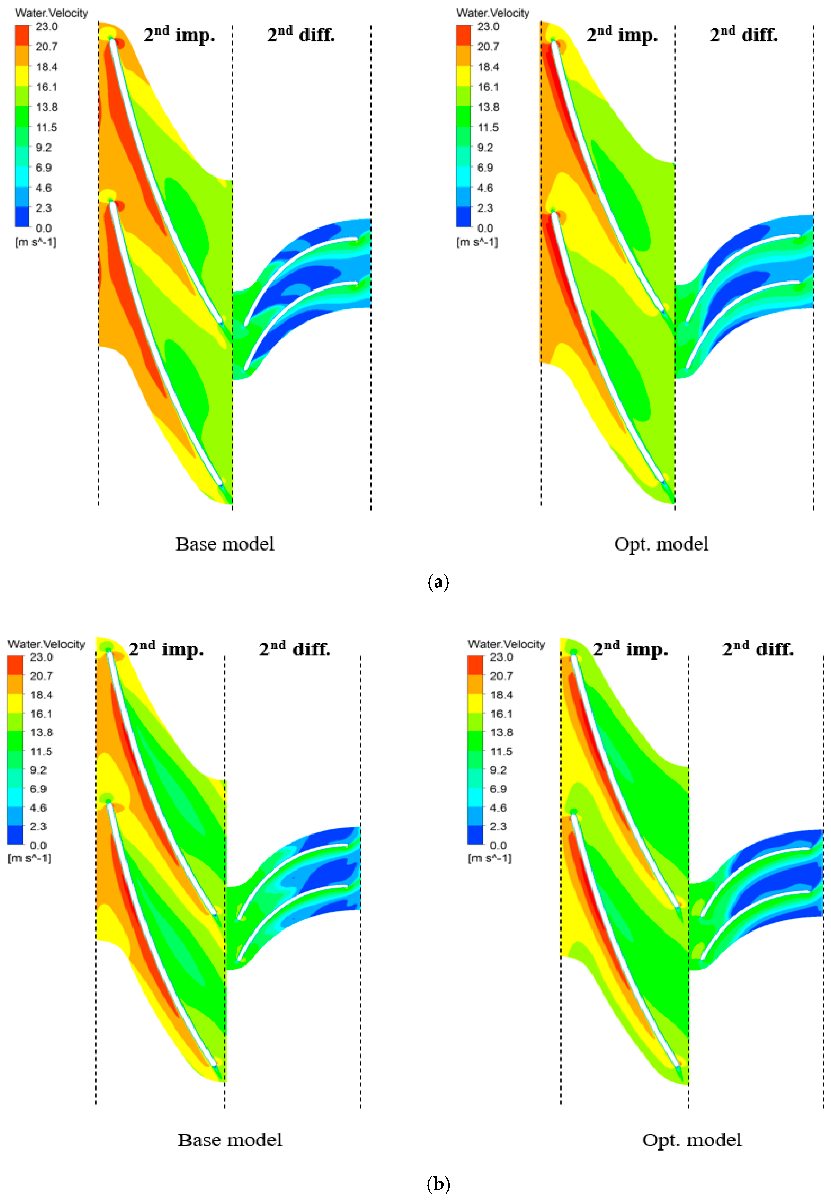
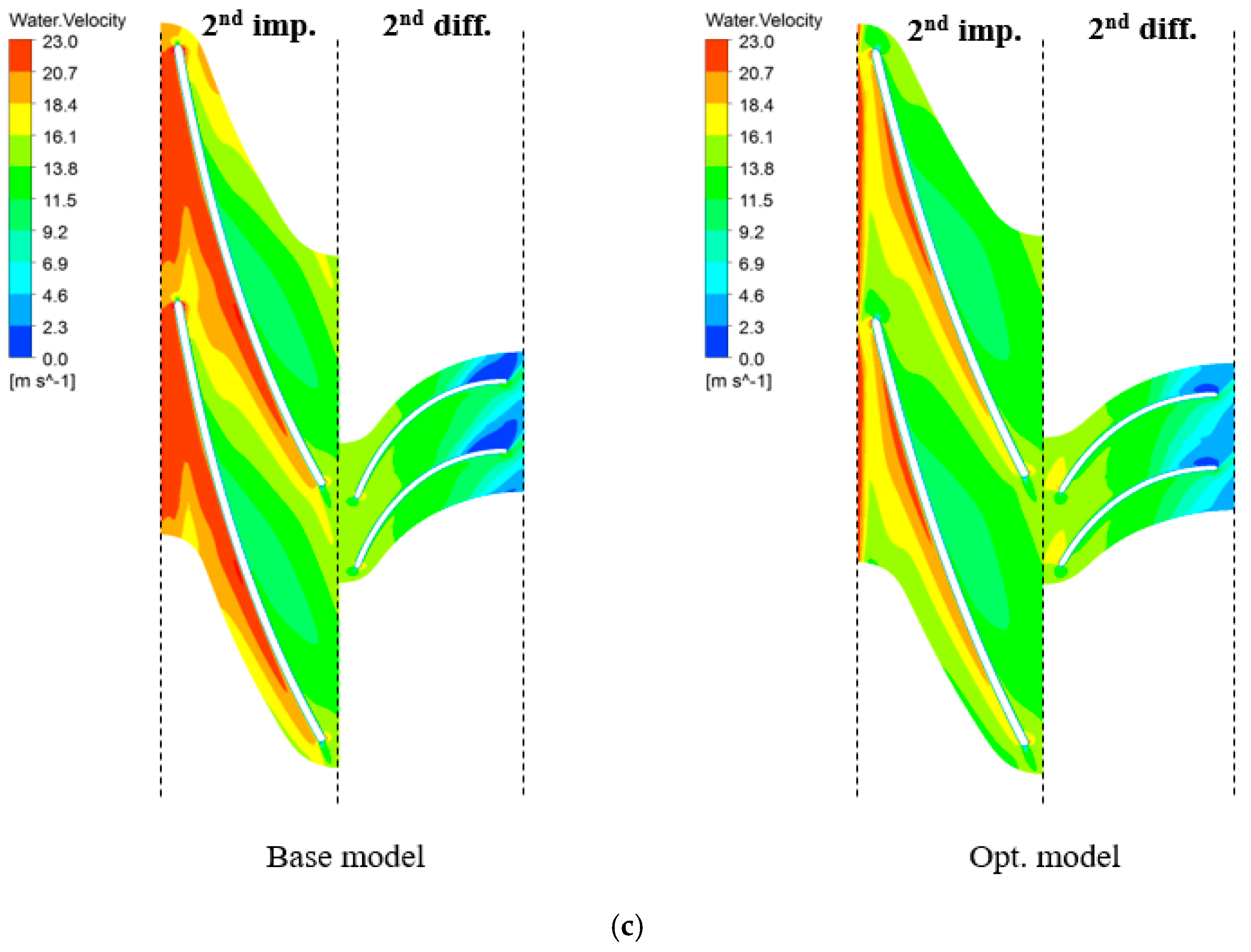
Figure 14 shows the velocity contours on the blade-to-blade passage at 20%, 50%, and 80% spans. In the base model, accelerating flow and a thin boundary layer on the suction side appeared in the impeller passage. Non-uniform flow was maintained along the streamwise direction, and a combination of the relative velocity and the blade’s rotational speed resulted in a high absolute velocity approaching the diffuser. Flow decelerated and the kinetic energy was transformed into internal energy with a resulting rise in static pressure, as the performance of the diffuser is dependent on the development of boundary layers during the deceleration process. In general, the diffuser was likely to separate from the blade under the action of the adverse pressure gradient. On the other hand, the optimum model showed nearly constant flow and relatively nominal boundary layers on the suction side along the spanwise direction. Moreover, the reduction in flow blockage and instability contributed to the improvement in static pressure recovery in comparison with the base model.

The above results might have been obtained because the flow angle and the blade angle matched well at the inlet and the outlet. These results show that total efficiency and pressure increased because of the optimization.

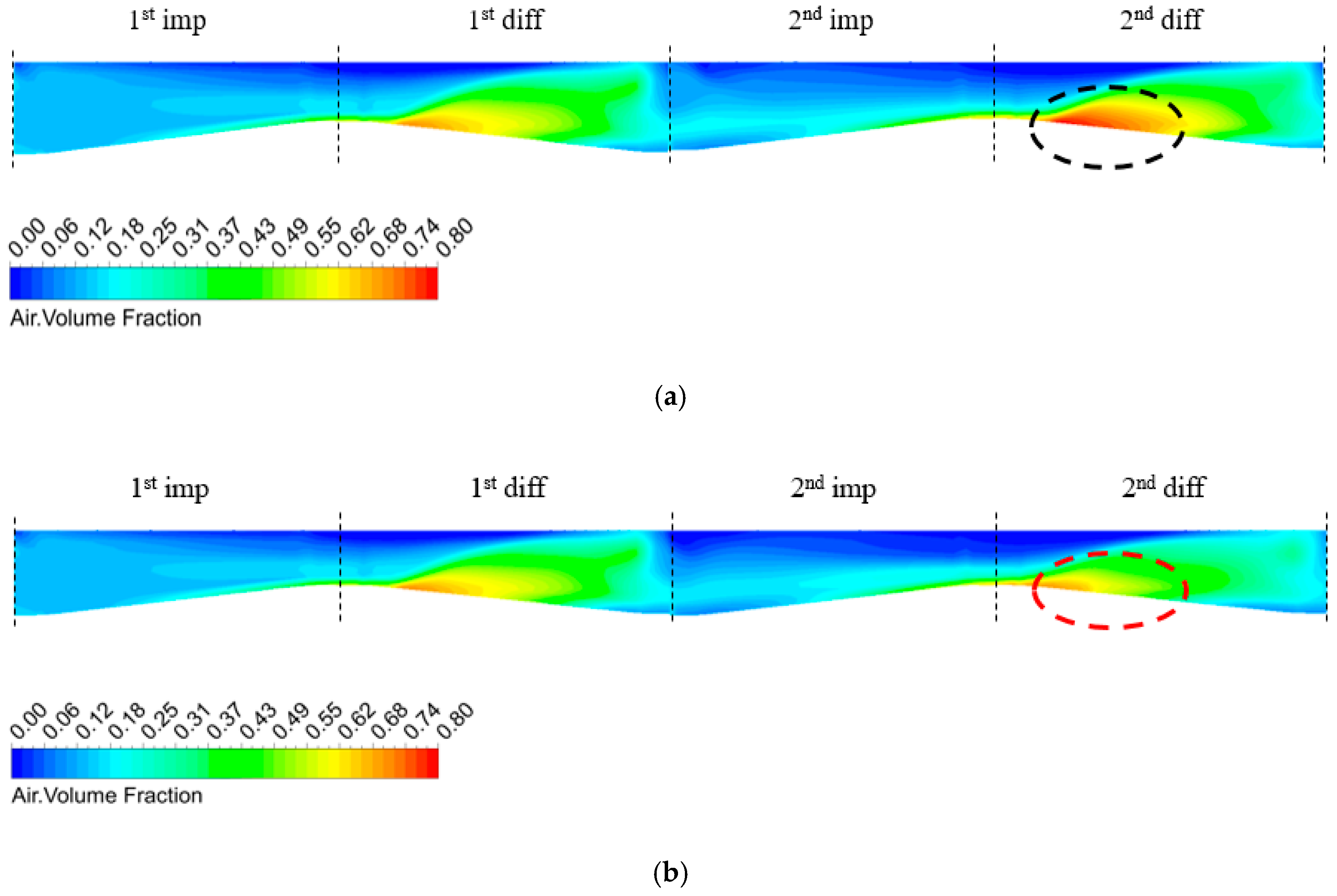
As shown in Figure 15, the air volume fraction on the meridional plane at GVF was 15%. The intensity of the air content in the flow accumulated first near the hub due to differences in the circumferential velocity and density between the phases of the impeller. The water and airflow exhibited a disordered flow pattern because of interactions between the rotating and the stationary domains, and flow blockage resulted from flow separation in the diffuser. The magnitude of phase separation at the optimum model was suppressed to a greater extent than that at the base model. It is believed that the greater pressure increments from compressive effects and the reduction of flow instability contributed to the improved phase mixing, static pressure recovery, and smooth flow movements.

6. Conclusions

In this study, the performance of a second-stage multi-phase pump was optimized using a systematic technique combined with a central composite method and a hybrid multi-objective evolutionary algorithm coupled with a surrogate model. Differences in flow characteristic were remarkable between the single-stage diffuser and the second-stage impeller. Due to the discordance between flow and the blade angles, the design variables of the impeller were selected to control both the inlet and the outlet angles in accordance with constraints. The selected design variables for the diffuser were the hub and the shroud inlet angle. The outlet angle of the diffuser was designed to decelerate flow and deflect it along the axis direction that increased the static pressure of the fluid. Therefore, the diffuser’s hub and shroud outlet angles were fixed at 90°. The multi-objective optimization of the second impeller and second diffuser were performed sequentially.

Based on the results of the numerical analysis of the test sets generated through CCD, regression analyses of the RSA surrogate model were conducted and multi-objective optimization was executed to obtain global POSs. Cluster_A (an efficiency-oriented model) was selected as the final model of the second-stage impeller. The calculated results were in agreement with the predicted values generated by the POSs, and represented better hydraulic performance compared with the base model. The total efficiency of Cluster_A increased by 1.1% and its total pressure by 16.3 kPa compared with the base impeller. The design optimization of the diffuser was also performed using the same process. The predicted performance in terms of static pressure and efficiency was estimated at 379.61 kPa and 63.25%, using the surrogate model and sequential quadratic programming, and was calculated to be 379.3 kPa and 63.22%, respectively. The static efficiency of the optimum diffuser increased by 3.1% and its static pressure by 27 kPa compared with the base model in single-phase flow. A comparison in terms of hydraulic performance between the base and the optimum models at design flow rate was conducted along the GVF ranges. As the increase in the size and number of bubbles caused them to be more closely spaced, this influenced the internal pressure with increasing GVF. An increase in static pressure and the static efficiency of the optimum model generally occurred along the GVF, up to 15% compared with the base model.

To determine the main factors responsible for the improvement in performance, internal flow fields for the base model and the optimum model were analyzed. It revealed problems caused by non-uniform flow due to discord between the flow angle and the blade angle from the inlet to the outlet in the base model. In the optimum model, the non-uniform flow was suppressed. Therefore, the improvement in performance was due to reduce 2D and 3D loss of the unshrouded impeller. Furthermore, the intensity of the air content in the flow accumulated first near the hub due to differences in circumferential velocity and density difference between phases in the impeller. The water and airflow exhibited a disordered pattern because of the interaction between the rotating and the stationary domains as well as the effect of flow blockage resulting from flow separation in the diffuser. The magnitude of phase separation in the optimum model was suppressed to a greater extent than that at the base model. It might have been that higher pressure increments from compressive effects and a reduction in flow instability contributed to the improved phase mixing, static pressure recovery, and smooth flow movements.

From the results of this work, three conclusions can be drawn: (1) it was confirmed that the proposed multi-objective optimization technique can simultaneously improve the pressure and efficiency of the multi-phase pump; (2) it provides greater understanding of the trade-off among multi-objective functions using design variables; (3) it provides guideline for economical solutions according to design conditions of multi-phase pumps.

References

1. Stel, H.; Sirino, T.; Ponce, F.J.; Chiva, S.; Morales, R.E.M. Numerical investigation of the flow in a multistage electric submersible pump. J. Pet. Sci. Eng. 2015, 136, 41–54. [Google Scholar] [CrossRef]
2. Zhang, J.; Li, Y.; Cai, S.; Zhu, H.; Zhang, Y. Investigation of gas–liquid two-phase flow in a three-stage rotodynamic multi-phase pump via numerical simulation and visualization experiment. Adv. Mech. Eng. 2016, 8, 1–13. [Google Scholar]
3. Nohmi, M.; Sakurai, T.; Sogawa, Y. Hydrodynamic design system for pumps based on 3D CAD, CFD, and inverse design method. ASME J. Fluids Eng. 2002, 124, 329–335. [Google Scholar]
4. Cao, S.; Peng, G.; Yu, Z. Hydrodynamic design of rotodynamic pump impeller for multi-phase pumping by combined approach of inverse design and CFD analysis. J. Fluids Eng. 2005, 127, 330–338. [Google Scholar] [CrossRef]
5. Zhang, J.; Zhu, H.; Yang, C.; Li, Y.; Wei, H. Multi-objective shape optimization of helico-axial multi-phase pump impeller based on NSGA-II and ANN. Energy Convers. Manag. 2011, 52, 538–546. [Google Scholar] [CrossRef]
6. Kim, J.H.; Kim, J.W.; Kim, K.Y. Axial-flow ventilation fan design through multi-objective optimization to enhance aerodynamic performance. J. Fluids Eng. 2011, 133, 101101. [Google Scholar] [CrossRef]
7. Suh, J.W.; Kim, J.H.; Choi, W.C.; Son, J.H.; Joo, W.G.; Yoon, J.Y.; Choi, Y.S. Validation for performance evaluation of multi-phase pump using CFD and experiment. In Proceedings of the ASME Verification and Validation Symposium, Las Vegas, NV, USA, 11–15 May 2015. Paper No. VVS2015-8034. [Google Scholar]
8. Kim, J.H.; Lee, H.C.; Kim, J.H.; Choi, Y.S.; Yoon, J.Y.; Yoo, I.S.; Choi, W.C. Improvement of Hydrodynamic Performance of a Multiphase Pump Using Design of Experiment Techniques. J. Fluids Eng. 2015, 137, 081301. [Google Scholar] [CrossRef]
9. Suh, J.W.; Kim, J.H.; Choi, Y.S.; Joo, W.G.; Lee, K.Y. A study on numerical optimization and performance verification of multi-phase pump for offshore plant. Proc. Inst. Mech. Eng. A J. Power Energy 2017, 231, 382–397. [Google Scholar] [CrossRef]
10. Suh, J.W.; Kim, J.H.; Kim, J.H.; Yoon, J.Y.; Joo, W.G.; Choi, Y.S. Design optimization to improve the performance of the second-stage impeller in a helico-axial pump. In Proceedings of the 13th Asian International Conference on Fluid Machinery, Tokyo, Japan, 7–10 September 2015. Paper No. AICFM13-109. [Google Scholar]
11. Suh, J.W.; Choi, Y.S.; Kim, J.H.; Joo, W.G.; Lee, K.Y. Multiphase flow analysis for air-water bubbly in multiphase pump. In Proceedings of the ASME 2017 Fluids Engineering Division Summer Meeting, Waikoloa, HI, USA, 30 July–3 August 2017. Paper No. FEDSM2017-69239. [Google Scholar]
12. Gülich, F.J. Centrifugal Pumps; Springer: Berlin, Germany, 2008. [Google Scholar]
13. Menter, F.R. Two-equation eddy-viscosity turbulence models for engineering applications. AIAA J. 1994, 32, 1598–1605. [Google Scholar] [CrossRef]
14. Afolabi, E.A.; Lee, J.G.M. Investigating the effect of air volume fraction on the velocity distributions of air-water flow in a pipe separator. Int. J. Sci. Adv. Technol. 2013, 3, 36–45. [Google Scholar]
15. Hassan, Y.A. Multiphase bubbly flow visualization using particle image velocimetry. Ann. N. Y. Acad. Sci. 2002, 972, 223–228. [Google Scholar] [CrossRef] [PubMed]
16. ANSYS CFX-17.1. ANSYS CFX Manager User’s Guide; Ansys Inc.: Canonsburg, PA, USA, 2016. [Google Scholar]
17. Enwald, H.; Peirano, E.; Almstedt, A.E. Eulerian two-phase flow theory applied to fluidization. Int. J. Multiph. Flow 1996, 22, 21–66. [Google Scholar] [CrossRef]
18. Grace, J.R.; Wairegi, T.; Nguyen, T.H. Shapes and velocities of single drops and bubbles moving freely through immiscible liquids. Chem. Eng. Res. Des. 1976, 54, 167–173. [Google Scholar]
19. Tomiyama, A. Struggle with computational bubble dynamics. Multiph. Sci. Technol. 1998, 10, 369–405. [Google Scholar]
20. Antal, S.P.; Lahey, R.T.; Flaherty, J.E. Analysis of phase distribution in fully developed laminar bubbly two-phase flow. Int. J. Multiph. Flow 1991, 17, 635–652. [Google Scholar] [CrossRef]
21. Lopez de Bertodano, M. Turbulent Bubbly Flow in a Triangular Duct. Ph.D. Thesis, Rensselaer Polytechnic Institute, Troy, NY, USA, 1991. [Google Scholar]
22. Sato, Y.; Sekoguchi, K. Liquid velocity distribution in two-phase bubbly flow. Int. J. Multiph. Flow 1975, 2, 79–95. [Google Scholar] [CrossRef]
23. Dixon, S.L.; Hall, C. Fluid Mechanics and Thermodynamics of Turbomachinery; Butterworth-Heinemann: Oxford, UK, 2013. [Google Scholar]
24. Japikse, D.; Baines, N. Introduction to Turbomachinery; Oxford University Press: Oxford, UK, 1994. [Google Scholar]
25. Barbara, B.; Joiner, B.; Cryer, J. Minitab Handbook: Updated for Release 14; Cengage Learning: Boston, MA, USA, 2004. [Google Scholar]
26. Box, G.E.; Hunter, W.G.; Hunter, J.S. Statistics for Experimenters: An introduction to Design, Data Analysis, and Model Building; John Wiley & Sons Inc.: New York, NY, USA, 1978. [Google Scholar]
27. Myers, R.H. Response Surface Methodology; Allyn and Bacon, Inc.: Boston, MA, USA, 1971. [Google Scholar]
28. Myers, R.H.; Montgomery, D.C. Response Surface Methodology: Process and Product Optimization Using Designed Experiments; John Wiley & Sons Inc.: New York, NY, USA, 2002. [Google Scholar]
29. Deb, K. Multi-Objective Optimization Using Evolutionary Algorithm; Wiley & Sons: New York, NY, USA, 2001. [Google Scholar]
30. MATLAB®. The Language of Technical Computing; The Math Works Inc.: Natick, MA, USA, 2004. [Google Scholar]
31. Guinta, A.A. Aircraft Multidisciplinary Design Optimization Using Design of Experimental Theory and Response Surface Modeling Methods. Ph.D. Thesis, Virginia Polytechnic Institute and State University, Blacksburg, VA, USA, 1997. [Google Scholar]
Figure 1. Helico-axial multiphase pump.
Energies 10 01334 g001
Figure 2. Numerical analysis domain and schemes.
Energies 10 01334 g002
Figure 3. Overall multi-objective optimization procedure.
Energies 10 01334 g003
Figure 4. Definition of design variables of the impeller.
Energies 10 01334 g004
Figure 5. Definition of design variables of the diffuser.
Energies 10 01334 g005
Figure 6. Training point of central composite design sets. (a) Design variables and ranges of impeller; (b) Design variables and ranges of diffuser.
Energies 10 01334 g006
Figure 7. Pareto-optimal frontiers within the design space.
Energies 10 01334 g007
Figure 8. Optimal angle distribution of the 2nd stage impeller.
Energies 10 01334 g008
Figure 9. Optimal solution with the result of training points.
Energies 10 01334 g009
Figure 10. Performance comparison of the base model and optimum model. (a) Gas volume fraction vs. static pressure rise; (b) Gas volume fraction vs. static efficiency.
Energies 10 01334 g010
Figure 11. Distributions of static pressure at 50% span along the streamwise location. (a) Gas Volume Fraction 0%; (b) Gas Volume Fraction 15%.
Energies 10 01334 g011
Figure 12. Velocity contour at mid-span along the GVF up to 15%. (a) 2nd base impeller at the blade to blade plane; (b) 2nd optimum impeller at the blade to blade plane.
Energies 10 01334 g012
Figure 13. Internal flow contours near the trailing edge of the 2nd impeller. (a) Location of observation; (b) total pressure contour; (c) velocity contour.
Energies 10 01334 g013
Figure 14. Velocity contour on the blade-to-blade passage. (a) At 20% span; (b) at 50% span; (c) at 80% span.
Energies 10 01334 g014aEnergies 10 01334 g014b
Figure 15. Air volume fraction on the meridional plane at GVF 15%. (a) 2nd base model; (b) 2nd optimum model.
Energies 10 01334 g015