Numerical and Experimental Investigation of Equivalence Ratio (ER) and Feedstock Particle Size on Birchwood Gasification


Department of Engineering and Sciences, University of Agder, Grimstad 4879, Norway
*
Author to whom correspondence should be addressed.
Energies 2017, 10(8), 1232; https://doi.org/10.3390/en10081232
Submission received: 13 July 2017
/
Revised: 11 August 2017
/
Accepted: 15 August 2017
/
Published: 19 August 2017
(This article belongs to the Special Issue Engineering Fluid Dynamics)
Abstract
:This paper discusses the characteristics of Birchwood gasification using the simulated results of a Computational Fluid Dynamics (CFD) model. The CFD model is developed and validated with the experimental results obtained with the fixed bed downdraft gasifier available at the University of Agder (UIA), Norway. In this work, several parameters are examined and given importance, such as producer gas yield, syngas composition, lower heating value (LHV), and cold gas efficiency (CGE) of the syngas. The behavior of the parameters mentioned above is examined by varying the biomass particle size. The diameters of the two biomass particles are 11.5 mm and 9.18 mm. All the parameters investigate within the Equivalences Ratio (ER) range from 0.2 to 0.5. In the simulations, a variable air inflow rate is used to achieve different ER values. For the different biomass particle sizes, CO, CO2, CH4, and H2 mass fractions of the syngas are analyzed along with syngas yield, LHV, and CGE. At an ER value of 0.35, 9.18 mm diameter particle shows average maximum values of 60% of CGE and 2.79 Nm3/h of syngas yield, in turn showing 3.4% and 0.09 Nm3/h improvement in the respective parameters over the 11.5 mm diameter biomass particle.
1. Introduction
Among the available energy sources, biomass is envisaged to play a major role in the future energy supplement. It produces no net carbon emission, while being the fourth largest energy source available in the world [1,2,3,4]. Therefore, biomass has high potential in contributing to satisfy the future energy demands of the world. Further, it is seen that for countries where the economy is mostly based on agriculture, they can utilize the potential of biomass efficiently. To recover energy from biomass, either thermochemical or biochemical process can be used [5,6,7]. The gasification process is a thermochemical process which gives a set of gases as output, consisting of CO, CO2, H2, CH4, and N2 by converting organic or carbonaceous materials like coal or biomass [8,9,10]. In gasification, several types of reactors used, such as entrained flow, fixed bed, fluidized bed, and moving bed gasifiers [7,11,12,13].
The producer gas is a result of a set of endothermic and exothermic reactions. The required heat for the endothermic reactions is provided by the exothermic reactions [11,14]. Once the steady state is achieved, the gasifier could work in a certain temperature range. Then, the producer gas can be obtained, as long as the fuel is being fed [14,15].
It was proven that producer gas was more versatile and useful than the biomass [16]. The quality of the producer gas is established to be one of the most important aspects of the gasification which should be enhanced, as it is used to generate power [11,16]. Chemical reactions inside the gasifier consist of both homogeneous and heterogeneous reactions. There are some factors which are important for the improvement of the gasification process such as reactor temperature, reactor pressure, the flow rate of the gasifying agent, and inflow rate of the biomass to the gasifier [11,17]. To evaluate gasification characteristics of biomass, a thorough evaluation is required. With the recent development of the computational fluid dynamics (CFD) and numerical simulations, sophisticated and robust models can be developed to give more qualitative information on biomass gasification [17,18]. In addition, CFD can produce important data with a relatively low cost [19]. Thus, CFD has become popular and an often-used tool to examine gasification characteristics [18,20,21].
Previous researches on gasification process have been performed on a regular basis investigating a broad range of parameters and variables. Most of them focused on the thermodynamics of the process, syngas composition, energy and exergy output, effect of temperature, the efficiency of the process, etc. [22,23]. Moreover, numerous numerical simulations have been done on the flow patterns and turbulence, as well as the different mathematical approaches. Ali et al. [24] developed a simulation model to discuss the co-gasification of coal and rice straw blend to investigate the syngas and cold gas efficiency (CGE), noting an 87.5% CGE value during the work. Slezak et al. [25] discussed an entrained flow gasifier using a CFD model to study the effects of coal particle density and size variations, where two devolatilization models were used in their work. It concluded that a higher fixed carbon conversion and H2 could be achieved with a mix of different partitioned coal. Rogel et al. [26] presented a detailed investigation on the use of Eulerian approaches on 1-D and 2-D CFD models to examine pine wood gasification in a downdraft gasifier. Syngas lower heating value, syngas gas composition, temperature profiles, and carbon conversion efficiency were investigated [26] for both models to conclude that these methods could be used effectively in determining the above-mentioned parameters. Sharma [17] developed a CFD model of a downdraft biomass gasifier to investigate the thermodynamic and kinetic modeling of char reduction reactions. Further, a conclusion has been made that char bed length is less sensitive to equilibrium predictions, while CO and H2 component, the calorific value of product gas and the endothermic heat absorption rate in reduction zone are found to be sensitive to the reaction temperature. Wu et al. [27] developed a 2-D CFD model of a downdraft gasifier to study the high-temperature agent biomass gasification, and observed a syngas with a high concentration of H2 with a limited need of combustion inside the gasifier. Janejreh et al. [28] discussed the evaluation of species and temperature distribution using a CFD model with k-ε turbulence model and Lagrangian particle models. The gasification process was assessed using the CGE. Ismail et al. [29] developed a 2-D CFD model by using the Eulerian-Eulerian approach. Coffee husks are used as the feedstock to model the gasification process of a fluidized bed reactor. The effect of Equivalence Ratio (ER) and moisture content on gasification temperature, syngas composition, CGE, and HHV were discussed. After the analysis, high moisture content of coffee husks was found as a negative impact on the CGE and Higher Heating Value (HHV) as the ER increased. Monteiro et al. [30] developed a comprehensive 2-D CFD model to examine the potential of syngas from gasification of Portuguese Miscanthus. The Eulerian-Eulerian approach was used to model the exchange of mass, energy, and momentum. For the work, the effect of ER, steam to biomass ratio and temperature on syngas quality assessed. ER was proven to be a positive impact on the Carbon Conversion Rate (CCE), where an adverse impact was shown on the syngas quality and LHV. Further, the syngas quality and gasification efficiency was found to be increased by the increasing temperature. In order to describe the gasification process of three Portuguese biomasses, Silva et al. [31] developed a 2-D CFD model. A k-ε model was used to model the gas phase, while an Eulerian-Eulerian approach was used to model the transport of mass, energy, and momentum. After the simulations, the highest CGE value was shown by vine-pruning residues, while a higher H2/CO ratio was shown by both coffee husks and vine pruning residues over the forest residues. Couto et al. [32] developed a 2-D CFD model using the Eulerian-Eulerian approach to evaluate the gasification of municipal solid waste. The gasification temperature was defined to be vastly important in syngas heating value in conclusion. In comparison to the above research works, the novelty of this study lies in the field of the Birchwood gasification. In addition, the literature lacks the use of 3-D CFD models and experiments on the effect of wood particle size on CGE. In this article, a 3-D CFD model is developed to investigate the Birchwood gasification in a fixed bed downdraft gasifier. Both heterogeneous and homogeneous reactions are considered and variation of syngas composition, syngas yield, LHV of the syngas, and CGE are measured for two sizes of feedstock, as well as for ER. Fixed bed downdraft gasifiers have demonstrated to perform well in the ER range from 0.25 to 0.43. Therefore, in the present work, the variations of the gasification parameters are considered in the ER range from 0.2 to 0.5 [14,15]. For the experimental work, the downdraft gasifier is used, which is available at the University of Agder (UIA), Norway. In addition, the CFD model is developed as the same geometry of the gasifier used for the experiments. For the validation purposes, experiments are done with the same gasifier with one of the wood particle sizes (11.5 mm woodchip) as it is the only biomass particle size available for the experiments. Then, with the developed simulation model, both biomass particle sizes are simulated.
2. Feedstock Characteristics
For the study, Birchwood is used as the feedstock. The ultimate and proximate analysis results for the Birchwood are listed down in Table 1. The data is extracted from a previous study [33], which is done on Birchwood in the same lab and under the same conditions.
According to the analysis above, Birchwood has a lower amount of moisture in comparison to some of the other wood types [33,34,35], which is an important aspect for gasification. Apart from the moisture content, Birchwood has shown a lower amount of ash, Cl, and S, while higher values of calorific value and volatile matter [34] has been indicated. It is obvious that Birchwood has a higher calorific value because of the higher amount of carbon content [33]. In addition, when a biomass consists of less ash, it can lead to a higher conversion process which has lesser slag [14]. Hence, Birchwood has some positive characteristics in the gasification perspective. According to some of the literature, K, Si, and Ca can have a small effect in determining gasification characteristics. However, in this work, those are not considered as they are not measured in the ultimate analysis [36].
3. Methods
In this section, first, the experimental setup and the experimental process is described. Then, a brief description of the equations which use for the calculations is presented. It is then followed by the numerical study and simulation process.
3.1. Experimental Study
For the experiment, initially, about 6 kg of biomass is fed into the gasifier along with 1 kg of charcoal. Charcoal is added to the system to help the ignition process. The simulations are also carried out following the same procedure. The average size of the Birchwood chip which was used for the experiments is approximately 11.5 mm × 11.5 mm. A schematic diagram of the system is shown in Figure 1.
The hopper is a conically shaped stainless-steel structure with a volume of 0.13 m3 and double-walled thick walls. It has a radius of 0.5 m. Biomass is fed through this hopper, and it is connected to an electrical shaker which can provide 15 shakes per minute (shakes/min). This shaking process helps to reduce or avoid some common problems, such as channeling and bridging. To drain out the condensed moisture, a drain valve is also attached to the bottom of the hopper.
The primary gasification reactor has a diameter of 0.26 m. It is 0.6 m in height. The air inlet system consists of six same size nozzles with equal spacing among each of a 5 mm diameter, and they are located from about 0.4 m from the bottom of the reactor. At the bottom of the reactor part, a reciprocally oscillating grate is connected and takes out the ash to the lower part of the ash collector. The grate is oscillating 30 s/min. To measure the weight loss during the gasification process, a mass scale locates at the bottom of the gasifier system. In addition, two pressure sensors and five K-type thermocouples are connected to the gasifier assembly to monitor and measure the parameters.
All the necessary experimental data is measured via a Lab view program which is specially designed to obtain data from the gasifier system. Further, to measure the composition of the syngas, a gas sample is sent to a gas analyzer, and throughout the experiment, changes in the composition of the syngas output is produced by the gas analyzer.
3.2. Theoretical and Numerical Study
In this study, the effect of biomass particle size and ER on the behavior of gasification parameters is examined using Birchwood as the feedstock. Thus, the variance of producer gas composition, producer gas yield, LHV of the syngas, and CGE is mainly assessed on two different values of biomass particle sizes.
Although downdraft gasifier demonstrates better performances at the ER ratio of 0.25, acceptable performances showed even close to the ER value of 0.43 [33,37]. Therefore, ER value range from 0.2 to 0.5 is selected in this study to investigate the best performance. ER is calculated using the following expression Equation (1) [8,15].
Since the Hydro-Carbons (HC) higher than CH4 are not considered for this study, they have not been used to calculate .
In the simulation model, a spherical particle is used for modeling. Hence, spherical particles with a diameter of 11.5 mm (available wood chip size in the lab) and 9.18 mm are utilized for the simulations (a spherical particle which has the same surface area as an actual wood chip, with a diameter of 9.18 mm consider here).
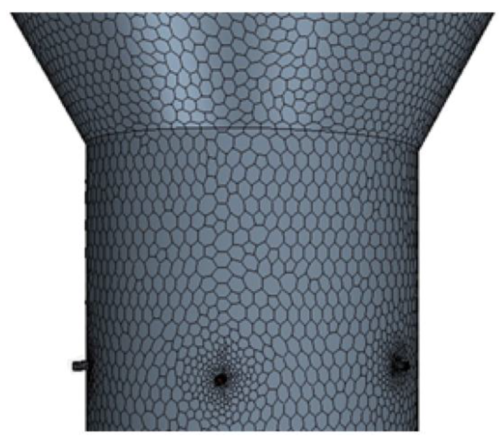
In the presented work, the STAR CCM+ software package is used for the modeling and simulation. A 3D geometric model of the actual gasifier is designed to create the computational model. For the gasifier model, 0.01m mesh is used, while in the air inlets and air-fuel mixing region, a 0.001 m mesh has been used. Figure 2 shows the customized meshfor the gasifier (0.01 m) and for air inlets (0.001 m).
A segregated flow model is implemented to solve the transport equations. In addition, the Lagrangian particle modeling method is used to model the particle behavior (solid phase).
3.2.1. Assumptions
The underlying assumptions of the modeling process are summarized as follows:
- Steady flow is considered inside the gasifier.
- The flow inside the domain is considered as incompressible and turbulent.
- Spherical particles are used.
- Evenly distributed particle regime is utilized.
- The No-slip condition is imposed on inside wall surfaces.
3.2.2. Eulerian-Lagrangian Method
Reynolds averaged Navier-Stokes (RANS) equations are solved using a Eulerian-Lagrangian reference frame to solve the numerical scheme. The gas phase is considered as a reacting gas phase, and Lagrangian particle models are used to address the solid (particle) phase. Standard k-ε model is used for turbulence modeling. In addition, both finite rates of chemical reactions and eddy dissipation rates are used in the computational model. Moreover, for the modeling work, the conservation equations for transport of energy, momentum, and mass are used (Appendix A). Also, the default sub models available for moisture evaporation, devolatilization and char oxidation are employed (Appendix A). In the Eulerian-Eulerian approach, gas phase, as well as the solid phase, is considered as continuum [41]. In the Lagrangian approach, usually a large number of particles are tracked transiently. The method is started by solving the transient momentum equation for each particle. In order to calculate the trajectory of a particle, Newton’s second law is used and written in a Lagrangian reference frame [41,42,43,44]. Momentum balance for particles is described in Equation (6),
where represents the velocity of the particle, is the mass of the particle, and is time. and represent the surface force and body force, respectively. When these forces are observed in depth, each of them is a composition of few forces available in the system. The following Equations (7) and (8) describe the two forces.
Using the Nusselt number (), the heat transfer coefficient can be found for the Lagrangian particle, which is the energy model for the Lagrangian particle. This is shown in Equation (10),
where has represented the thermal conductivity of the phase and is the particle diameter. Nusselt number () is expressed in the following Equation (11), where it is calculated by the Ranz-Marshall correlation and presented below in Equation (12).
3.2.3. Reactions Modeling
In this work, the following approach is used to simulate the gasification process. This method has been used by [8,48]. In this study, it is assumed that the moisture is evaporated completely in the drying phase [49].
In the pyrolysis phase, the Biomass (dry) is converted into char, tar, ash, and volatile matter [49,50].
Here, the volatile matter is described as follows. It is assumed that the volatile matter consists of only CO, CO2, H2, and CH4.
The following method is used to calculate the mass distribution in volatile matter and mass fractions in dry biomass. For the calculations, the data available in Table 1 is used. These values can be used to combine with the ultimate analysis. In this method, a set of linear equations is used to solve the C, O, and H components balance in the system [8,48].
In the above equations, the coefficients are the ratios of molar mass of each atom to the molar mass of each species. (As an example, in Equation (15), ). Here, with the molar masses, the numerical values are rounded up for the simplification of the calculations. For finding the mass fractions , , and , the following method is used along with the data from the ultimate analysis of the biomass.
According to the mass conservation,
Thus, according to the above criteria,
The ratio between CO and CO2 is temperature dependent. In this study, the ratio has been determined as 2.43 according to [8]. For the calculations, the bed temperature is used as 907 K, which was obtained during the experiments. Below Equation (21) is used to determine the connection between CO and CO2 at 907 K.
The linear equations from Equation (9) to Equation (15) are solved using the MATLAB program, and the following values are obtained from the program.
According to the above results, 1 kg of volatile matter produce devolatilized products according to the following expression.
Using the following molar mass values, the above Equation (23) can be used as a molar based equation.
Therefore, according to the following (R4), the devolatilization of the volatiles is modeled.
Based on the above devolatilization reaction (R4), the gasification process is modeled. In addition, for the modeling work, the following homogeneous and heterogeneous reactions are considered [8,28,51].
Water-gas shift reaction:
Methanation reaction:
Dry reforming reaction:
Steam reforming reaction:
mbustion reaction:
Boudouard reaction:
Water-gas reaction:
Hydrogasification:
Carbon partial reaction:
4. Results and Discussions
In this section, the computational model validation is conducted by comparing the available experimental data and numerical simulation results. Moreover, the comparison of the two sizes of biomass particle sizes is carried out using the gasification characteristics.
4.1. Development of Mass Fractions of Considered Gases in the Syngas
A specially designed lab view program was used to measure all the gas component mass fractions throughout the experiment. From the obtained data, the variation of the mass fractions of the gas components during the experiment is presented below in Figure 3. For the tests, a biomass woodchip with an average size of 11.5 mm × 11.5 mm is used, which is available in the laboratory.
In the simulation model, for two iterations, one data point has been recorded. 600 iterations are used in the simulations, and 300 data points are recorded throughout the simulation. Using the obtained data points gas component mass fractions are graphed in Figure 4. For the simulations, two types of wood particle sizes are used. One of them is 11.5 mm in diameter, while the other is 9.18 mm in diameter. Below, Figure 4 was obtained using 11.5 mm diameter wood particle.
By comparing Figure 3 and Figure 4, it shows the fluctuation in gas components mass friction in the simulation values, whereas in the experiment, it shows smooth variation. It can be due to the fact that the interval between two data points are bigger. However, an average value is used to plot graphs.
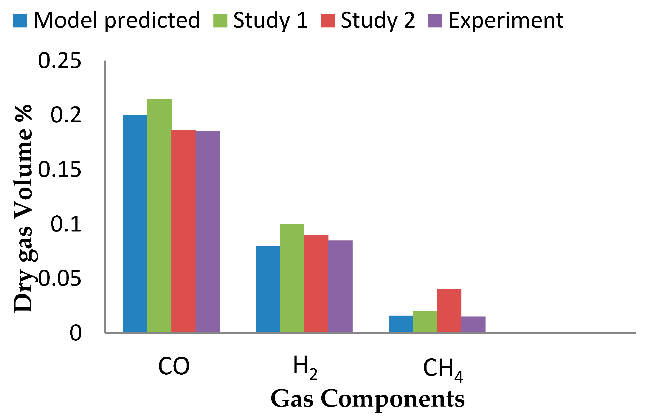
The data obtained from the model is also compared with some of the data collected from the literature (Study 1 [52], and Study 2 [53]), as well as with the data achieved during the experiment of the present work. Figure 5 shows the comparison of the predicted data along with the experimental data. According to the graph, predicted data shows good agreement with the literature and experimental data.
4.2. Effect of ER and Biomass Particle Size on Quality of Producer Gas
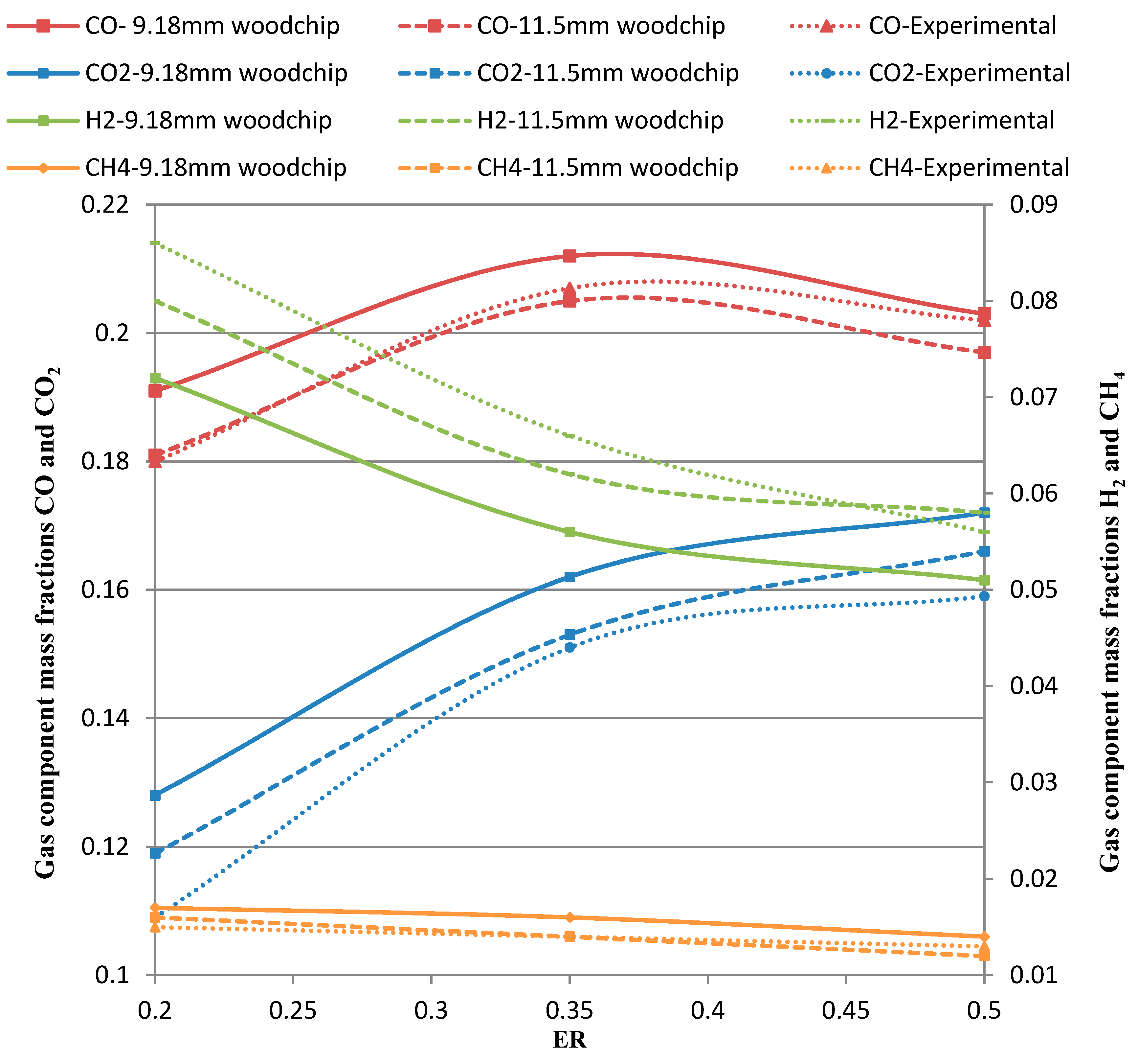
The variation of gas components in producer gas in both experiments and simulation models is illustrated in the following Figure 6. For the simulations, a biomass particle with a diameter of 11.5 mm and a biomass particle with a diameter of 9.18 mm were used. (The change of gas component contours in various ER values are illustrated in Appendix A (Figure A1, Figure A2 and Figure A3)).
According to Figure 6, mass fractions of CO and CO2 are increased when the ER is increased up to a certain level (ER = 0.2 to 0.35). Then, ER contributes to a reduction of the mass fraction of CO, while further increasing CO2. This can be a result of the combined effect of Combustion reaction (R9), Boudouard reaction (R10), and Carbon partial reaction (R13). Therefore, in lower ER values, (R10) tends to produce more CO to the system at the expense of CO2, while in high ER values, (R9) and (R13) convert more CO into CO2 [2].
Rgearding CH4 and H2, increasing ER is effected on a decrease in both gas species. Nevertheless, H2 is varied in a higher mass fraction range than of CH4. This is mainly due to the effects of dry reforming (R7) and steam reforming (R8) reactions, which produce more H2 to the system at the expense of CH4.
Since a variable air inflow rate is used in the experiments, an average value of the air inflow rate is used for the calculation of ER values. However, a fixed air inflow rate is used in the simulations. Therefore, the impact of variable air inflow may have caused the deviation in the graphs of the experimental and simulation data. In the simulations, spherical shape wood particles are used, while wood chips with different shapes are used for the experiments. The difference of behavior of spherical wood particle and divergement shaped wood chips can also create the inequalities in the graphs. In addition, during the experiments, channeling and bridging can also have taken place [7]. The effect of that phenomenon may have also affected the experimental results.
According to Figure 6, all the considered gas component mass fractions, except H2, are increased for the 9.18 mm wood particle over 11.5 mm wood particle. This pattern can be found in some of the literature [54,55]. When the particle size is getting smaller, the area to volume ratio of the wood particle is increased. This can result in an increased contact with the reactants [54,55,56]. Hence, the reaction rates can be increased and gasification reactions can also be improved. Further, the enhancement of hydrogasification (R12) is crucial for the behavior of the gas component mass fractions. When the biomass particle is getting smaller, it can enhance the reactivity and produce more CH4 with R12.
4.3. Effect of Equivalences Ratio (ER) and Biomass Particle Size on Syngas Yield, Lower Heating Value (LHV), and Cold Gas Efficiency (CGE)
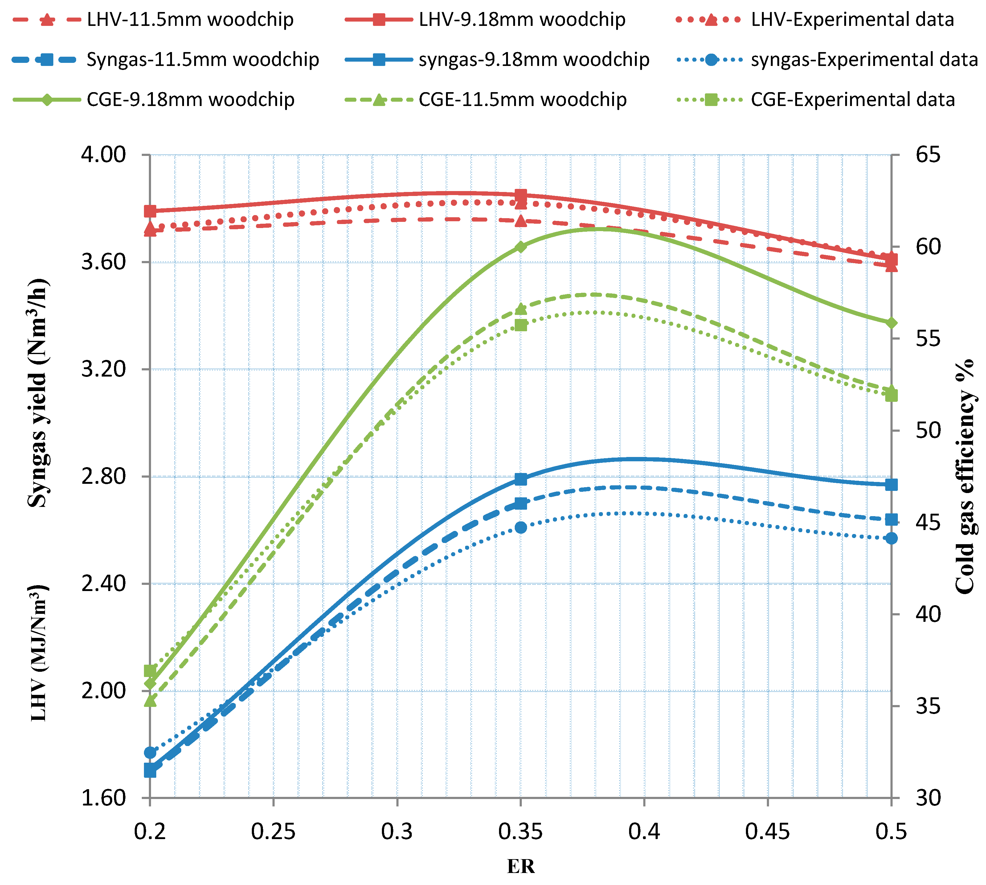
Figure 7 shows the variation of syngas yield, LHV and CGE of the syngas as a function of ER. According to Figure 7, the behavior of syngas yield could be an effect of higher volatilization [28].
During the simulations, both biomass particles are evaluated in the same ER range. However, the gas yields with two separate sizes of biomass particles have shown a difference. This difference of syngas yield should be due to a different conversion. For the context of LHV of syngas, increasing ER has shown a positive effect within the range from 0.2 to 0.35. It is evident that, as the gas species mass fractions increase, LHV of syngas increases as well.
According to Figure 7, the smaller particle size has resulted in a significant increment of the LHV of the gas, although it has followed the same variation along the ER range as the bigger biomass particle. The increment of LHV can be mainly due to the increment of CH4 with the smaller biomass particle. As mentioned before, LHV is a direct function of combustible gas species, and CH4 has the highest contribution for the LHV among the gas species.
For CGE, a positive effect of increasing ER is observed from 0.2 to 0.35 of ER. Within this ER range, CGE could have been improved by increasing airflow. Increasing airflow (increasing ER) can contribute to creating a high composition of combustible gas species in syngas by enhancing the reaction chemistry of homogeneous and heterogeneous reactions. Therefore, as the gas species are increased up to 0.35 of ER, so does the CGE. As the gas species have shown a decrement in the mass fractions in the ER range from 0.35 to 0.5, CGE has also shown a decrement in its value. With more O2 input to the system, the system can move towards combustion rather than gasification. This can be a result of the reduction of CGE after the ER value of 0.35. According to the graph in Figure 7, with the 9.18 mm biomass particle, CGE has shown an average maximum value of 60% at ER value of 0.35, compared to an average maximum value of 56.63 % with 11.5 mm diameter biomass particle.
For both particle sizes, same ER range is considered. Hence, an increase of LHV, syngas yield, and combustible gas spices in syngas with smaller biomass particle could be the reason for the increase of the CGE.
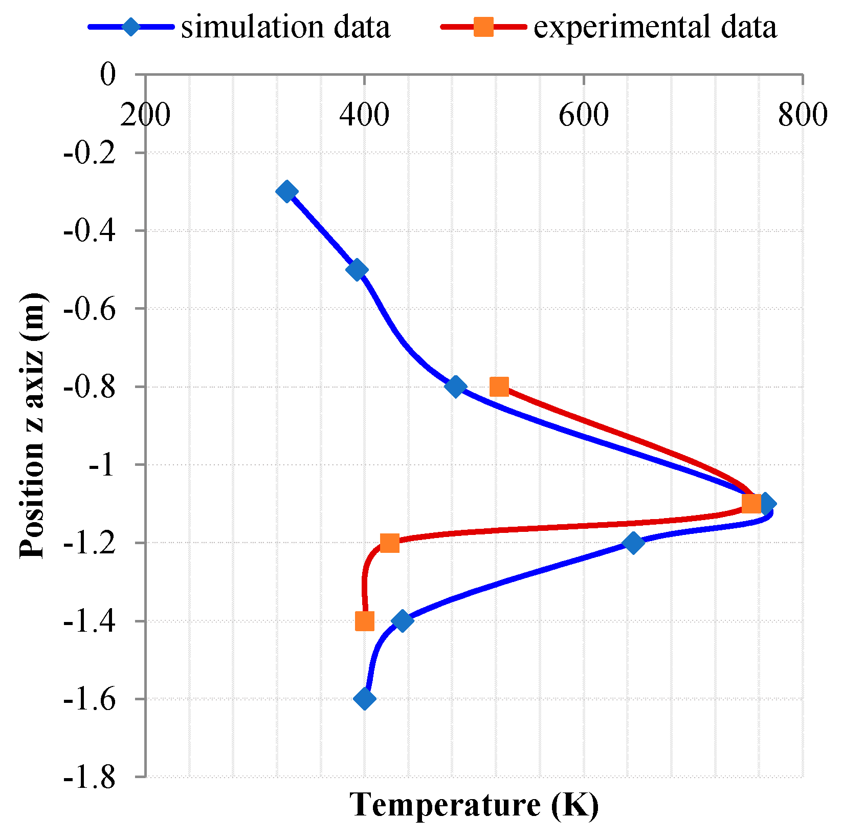
4.4. Temperature Profile
Temperature profile inside the gasifier in the simulation model is illustrated in Figure 8. In Figure 9, the temperature values recorded in the experiments and the simulation model are demonstrated in a graph. Figure 8 is mainly used to help understand the actual placement of the thermocouples. In the simulation model, seven temperature measurements are taken along the mid-axis, which is shown in Figure 9. However, in the experimental setup, only four thermocouples are available. Hence, to develop the curve, those four temperature measurement values are used. According to Figure 9, the maximum temperature is shown close to the air inlets in both experimental and simulation setups. In the experimental setup, the thermo couples are placed on the gasifier wall. Hence, the actual temperature can be slightly higher than what it is shown here.
5. Conclusions
Based on the comparative study, it is concluded that most of the measured and calculated parameters (including syngas yield, LHV of syngas, and CGE) have shown an increasing trend as ER is increased up to 0.35, and when biomass particle size is reduced. Furthermore, the average value of CGE, for instance, reached a maximum value of 60% with the 9.18 mm diameter wood particle, and with a corresponding ER about 0.35. Moreover, 11.5 mm diameter wood particle has shown an average maximum value of 56.6% at the same ER value, which has been both an improvement and a significant output of this work. Reaching an average value of 2.79 Nm3/h with a corresponding ER of 0.35, the average value of Syngas yield has shown an improvement of 0.09 Nm3/h with the 9.18 mm diameter wood particle over 11.5 mm wood particle, which has been an important aspect in energy harvesting from the syngas. Therefore, as the result shows, an ER value close to 0.35 shows the best results in CGE, syngas yield, and LHV of the syngas. Furthermore, smaller biomass particles show improvements in the results. Therefore, according to our study, in order to obtain better outputs, ER should be kept close to 0.35. In the future, more simulations and experiments could be done with finer biomass particles. Further, more user defined functions could be used to improve the gasification process and to represent more realistic biomass particle shapes.
Acknowledgments
Authors would like to thank Department of Engineering and Sciences, UiA, for supporting to do the experiment at Bio-energy lab. In addition, we would appreciate the contribution and guidance given by Hans Jorgen Morch, CEO of CFD Marine AS, especially in obtaining the license for the STAR CCM+ software.
Author Contributions
Rukshan Jayathilake and Souman Rudra conceived and designed the experiments; Rukshan Jayathilake performed the experiments; Rukshan Jayathilake and Souman Rudra analyzed the data; Rukshan Jayathilake and Souman Rudra wrote the paper.
Conflicts of Interest
The authors declare no conflict of interest.
Appendix A
Appendix A.1. Conservation Equations
In order to develop the numerical model, conservation equations have been used, along with some other important equations. The equation for mass conservation is presented below in Equation (A1) [39],
where is the density of the fluid, is the velocity tensor in the compact form in Einstein notation, t represents the time, and represents the special first order tensor.
The momentum conservation equation is:
where is the density of the fluid and is the gravity force. P represents the pressure, while the dynamic viscosity is represented by .
The energy equation is presented below in Equation A3 [57],
where represents the density of the fluid represents the pressure, k represents the thermal conductivity, and represents the viscous stress tensor.
Appendix A.2. Submodels
Appendix A.2.1. Two Ways Coupling
When the Lagrangian particles are relatively smaller, a one-way coupling model is used, since the heat transfer and drag force are the only things which affect through continues phase. However, once the particle size is much larger compared to the volume cells, then a more advance model has to be introduced. Once the two-way coupling is used, an active particle or the Lagrangian phase can exchange mass momentum and energy with fluid phase [58,59,60].
Appendix A.2.2. Coal Combustion Model
Coal combustion model is a set of sub models consist of moisture evaporation, two step devolatilization, and char oxidation models. Thus, in the following part, each of these models will be discussed.
Appendix A.2.3. Moisture Evaporation Model
The evaporation model has been built on a small assumption. It assumes the moisture has covered the whole particle with a thin film. According to that, the moisture has to be evaporated before the volatiles are released because moisture is at the outermost layer. In this model, there are no properties associated. Here, the Ranz Marshall correlation has been used to calculate the relevant Nusselt and Sherwood numbers. In order to formulate this model, the Quasi-Steady single component droplet evaporation model has been applied to a water droplet [61].
Appendix A.2.4. Devolatilization Model
In order to simulate the volatile release from the coal particles, a devolatilization model has to be used. In STAR CCM+, there are two devolatilization models that can be found: the single step devolatilization model and two step devolatilization models [46]. In Equation (A4), the devolatilization model for n steps has been shown.
In the above equation, represents the amount of char in the particle, while represents the volatile matter in the proximate analysis. The kinetic rate for the above equation is shown in the below Equation (A5).
represents the activation energy of the nth reaction for the particle and is the pre-exponential factor for the reaction. is the particle temperature, while is the universal gas constant. For the modeling work a single step devolatilization model is used. Hence, the pre-exponent factor and activation energy of is used for the study, which are generally used as the pre-exponent and activation energy values for wood [62].
Appendix A.3. Figures
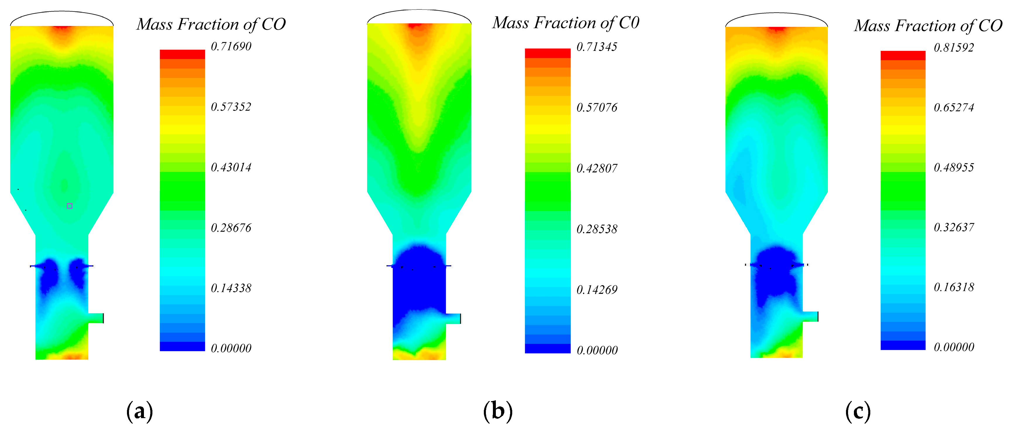
In the following Figure A1, change in CO contours against various ER values are shown.
Figure A1.
CO contours with ER values of (a) 0.2; (b) 0.35; (c) 0.5 from left to right.

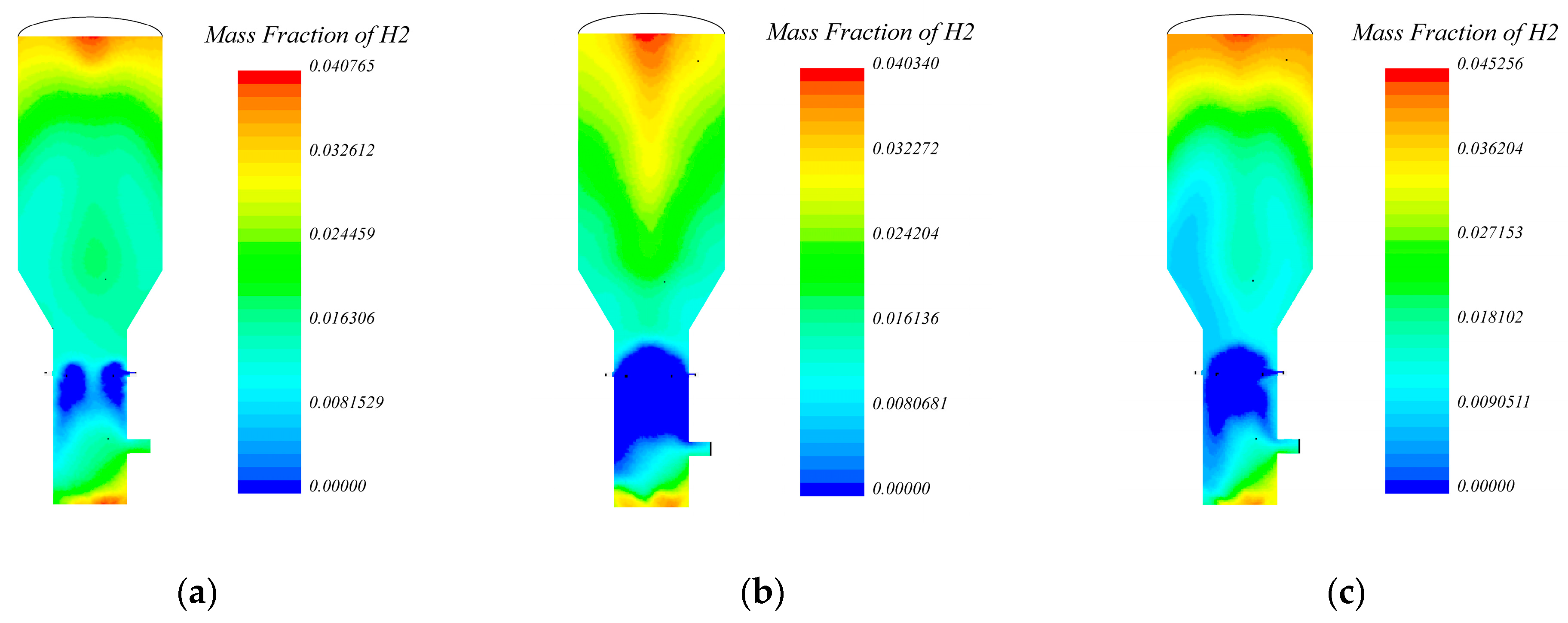
In the following Figure A2, change in H2 contours against various ER values are shown.
Figure A2.
H2 contours with ER values of (a) 0.2; (b) 0.35; (c) 0.5 from left to right.
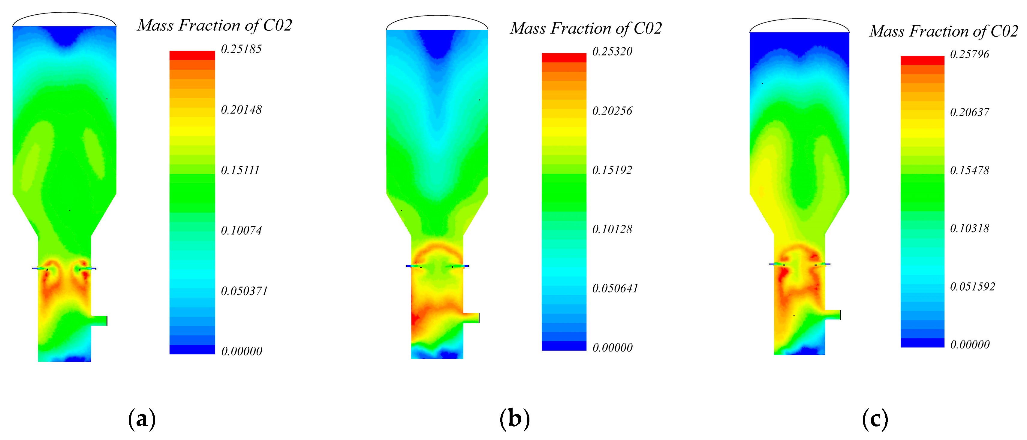
In the following Figure A3, change in CO2 contours against various ER values are shown.
Figure A3.
CO2 contours with ER values of (a) 0.2; (b) 0.35; (c) 0.5 from left to right.
References
- Caliandro, P.; Tock, L.; Ensinas, A.V.; Marechal, F. Thermo-economic optimization of a solid oxide fuel cell-gas turbine system fuelled with gasified lignocellulosic biomass. Energy Convers. Manag. 2014, 85, 764–773. [Google Scholar] [CrossRef]
- Sarker, S.; Bimbela, F.; Sánchez, J.L.; Nielsen, H.K. Characterization and pilot scale fluidized bed gasification of herbaceous biomass: a case study on alfalfa pellets. Energy Convers. Manag. 2015, 91, 451–458. [Google Scholar] [CrossRef]
- Saxena, R.C.; Adhikari, D.K.; Goyal, H.B. Biomass-based energy fuel through biochemical routes: A review. Renew. Sustain. Energy Rev. 2009, 13, 167–178. [Google Scholar] [CrossRef]
- Neri, E.; Cespi, D.; Setti, L.; Gombi, E.; Bernardi, E.; Vassura, I.; Passarini, F. Biomass Residues to Renewable Energy: A Life Cycle Perspective Applied at a Local Scale. Energies 2016, 9, 922. [Google Scholar] [CrossRef]
- Cotana, F.; Cavalaglio, G.; Coccia, V.; Petrozzi, A. Energy opportunities from lignocellulosic biomass for a biorefinery case study. Energies 2016, 9, 748. [Google Scholar] [CrossRef]
- Cavalaglio, G.; Gelosia, M.; D’Antonio, S.; Nicolini, A.; Pisello, A.L.; Barbanera, M.; Cotana, F. Lignocellulosic ethanol production from the recovery of stranded driftwood residues. Energies 2016, 9, 634. [Google Scholar] [CrossRef]
- Alauddin, Z.A.B.Z.; Lahijani, P.; Mohammadi, M.; Mohamed, A.R. Gasification of lignocellulosic biomass in fluidized beds for renewable energy development: A review. Renew. Sustain. Energy Rev. 2010, 14, 2852–2862. [Google Scholar] [CrossRef]
- Basu, P. Biomass Gasification and Pyrolysis: Practical Design and Theory; Academic Press: Burlington, MA, USA, 2010. [Google Scholar]
- Rudra, S.; Rosendahl, L.; Blarke, M.B. Process analysis of a biomass-based quad-generation plant for combined power, heat, cooling, and synthetic natural gas production. Energy Convers. Manag. 2015, 106, 1276–1285. [Google Scholar] [CrossRef]
- Zaccariello, L.; Mastellone, M.L. Fluidized-bed gasification of plastic waste, wood, and their blends with coal. Energies 2015, 8, 8052–8068. [Google Scholar] [CrossRef]
- Baruah, D.; Baruah, D.C. Modeling of biomass gasification: A review. Renew. Sustain. Energy Rev. 2014, 39, 806–815. [Google Scholar] [CrossRef]
- James, R.A.M.; Yuan, W.; Boyette, M.D. The effect of biomass physical properties on top-lit updraft gasification of woodchips. Energies 2016, 9, 283. [Google Scholar] [CrossRef]
- Shi, H.; Si, W.; Li, X. The concept, design and performance of a novel rotary kiln type air-staged biomass gasifier. Energies 2016, 9, 67. [Google Scholar] [CrossRef]
- Rajvanshi, A.K.; Goswami, D.Y. Biomass Gasification in Alternative Energy in Agriculture Vol. II; CRC Press: Boca Raton, FL, USA, 1986. [Google Scholar]
- Brown, R.C.; Stevens, C. Thermochemical Processing of Biomass: Conversion into Fuels, Chemicals and Power; Wiley series in Renewable Resources: Chichester, UK, 2011. [Google Scholar]
- Sheth, P.N.; Babu, B.V. Experimental studies on producer gas generation from wood waste in a downdraft biomass gasifier. Bioresour. Technol. 2009, 100, 3127–3133. [Google Scholar] [CrossRef] [PubMed]
- Sharma, A.K. Equilibrium and kinetic modeling of char reduction reactions in a downdraft biomass gasifier: A comparison. Sol. Energy 2008, 82, 918–928. [Google Scholar] [CrossRef]
- Wang, Y.; Yan, L. CFD studies on biomass thermochemical conversion. Int. J Mol. Sci. 2008, 9, 1108–1130. [Google Scholar] [CrossRef] [PubMed]
- Gerber, S.; Behrendt, F.; Oevermann, M. An Eulerian modeling approach of wood gasification in a bubbling fluidized bed reactor using char as bed material. Fuel 2010, 89, 2903–2917. [Google Scholar] [CrossRef]
- Ku, X.; Li, T.; Løvås, T. CFD-DEM simulation of biomass gasification with steam in a fluidized bed reactor. Chem. Eng. Sci. 2015, 122, 270–283. [Google Scholar] [CrossRef] [Green Version]
- Biglari, M.; Liu, H.; Elkamel, A.; Lohi, A. Application of scaling-law and CFD modeling to hydrodynamics of circulating biomass fluidized bed gasifier. Energies 2016, 9, 504. [Google Scholar] [CrossRef]
- Patel, K.D.; Shah, N.K.; Patel, R.N. CFD Analysis of spatial distribution of various parameters in downdraft gasifier. Procedia Eng. 2013, 51, 764–769. [Google Scholar] [CrossRef]
- Gerun, L.; Paraschiv, M.; Vijeu, R.; Bellettre, J.; Tazerout, M.; Gøbel, B.; Henriksen, U. Numerical investigation of the partial oxidation in a two-stage downdraft gasifier. Fuel 2008, 87, 1383. [Google Scholar] [CrossRef] [Green Version]
- Ali, D.A.; Gadalla, M.A.; Abdelaziz, O.Y.; Hulteberg, C.P.; Ashour, F.H. Co-gasification of coal and biomass wastes in an entrained flow gasifier: Modelling, simulation and integration opportunities. J. Nat. Gas Sci. Eng. 2017, 37, 126–137. [Google Scholar] [CrossRef]
- Slezak, A.; Kuhlman, J.M.; Shadle, L.J.; Spenik, J.; Shi, S. CFD simulation of entrained-flow coal gasification: Coal particle density/sizefraction effects. Powder Technol. 2010, 203, 98–108. [Google Scholar] [CrossRef]
- Rogel, A.; Aguillon, J. The 2D Eulerian approach of entrained flow and temperature in a biomass stratified downdraft gasifier. Am. J. Appl. Sci. 2006, 3, 2068–2075. [Google Scholar] [CrossRef]
- Wu, Y.; Zhang, Q.; Yang, W.; Blasiak, W. Two-dimensional computational fluid dynamics simulation of biomass gasification in a downdraft fixed-bed gasifier with highly preheated air and steam. Energy Fuels 2013, 27, 3274–3282. [Google Scholar] [CrossRef]
- Janajreh, I.; Al Shrah, M. Numerical and experimental investigation of downdraft gasification of wood chips. Energy Convers. Manag. 2013, 65, 783–792. [Google Scholar] [CrossRef]
- Ismail, T.M.; El-Salam, M.A.; Monteiro, E.; Rouboa, A. Eulerian-Eulerian CFD model on fluidized bed gasifier using coffee husks as fuel. Appl. Therm. Eng. 2016, 106, 1391–1402. [Google Scholar] [CrossRef]
- Monteiro, E.; Ismail, T.M.; Ramos, A.; El-Salam, M.A.; Brito, P.S.D.; Rouboa, A. Assessment of the miscanthus gasification in a semi-industrial gasifier using a CFD model. Appl. Therm. Eng. 2017, 123, 448–457. [Google Scholar] [CrossRef]
- Silva, V.; Monteiro, E.; Couto, N.; Brito, P.; Rouboa, A. Analysis of syngas quality from portuguese biomasses: An experimental and numerical study. Energy Fuels 2014, 28, 5766–5777. [Google Scholar] [CrossRef]
- Couto, N.D.; Silva, V.B.; Monteiro, E.; Rouboa, A. Assessment of municipal solid wastes gasification in a semi-industrial gasifier using syngas quality indices. Energy 2015, 93, 864–873. [Google Scholar] [CrossRef]
- Sarker, S.; Nielsen, H.K. Preliminary fixed-bed downdraft gasification of birch woodchips. Int. J. Environ. Sci. 2015, 12, 2119. [Google Scholar] [CrossRef]
- Sarker, S.; Nielsen, H.K. Assessing the gasification potential of five woodchips species by employing a lab-scale fixed-bed downdraft reactor. Energy Convers. Manag. 2015, 103, 801–813. [Google Scholar] [CrossRef]
- Atnaw, S.M.; Sulaiman, S.A.; Yusup, S. Influence of fuel moisture content and reactor temperature on the calorific value of syngas resulted from gasification of oil palm fronds. Sci. World J. 2014, 2014, 121908. [Google Scholar] [CrossRef] [PubMed]
- Bouraoui, Z.; Jeguirim, M.; Guizani, C.; Limousy, L.; Dupont, C.; Gadiou, R. Thermogravimetric study on the influence of structural, textural and chemical properties of biomass chars on CO2 gasification reactivity. Energy 2015, 88, 703–710. [Google Scholar] [CrossRef]
- Zainal, Z.A.; Ali, R.; Lean, C.H.; Seetharamu, K.N. Prediction of performance of a downdraft gasifier using equilibrium modeling for different biomass materials. Energy Convers. Manag. 2001, 42, 1499–1515. [Google Scholar] [CrossRef]
- Sarkar, M.; Kumar, A.; Tumuluru, J.S.; Patil, K.N.; Bellmer, D.D. Gasification performance of switchgrass pretreated with torrefaction and densification. Appl. Energy 2014, 127, 194–201. [Google Scholar] [CrossRef]
- Syed, S.; Janajreh, I.; Ghenai, C. Thermodynamics equilibrium analysis within the entrained flow gasifier environment. Int. J. Therm. Environ. Eng. 2012, 4, 47–54. [Google Scholar] [CrossRef]
- Renganathan, T.; Yadav, M.V.; Pushpavanam, S.; Voolapalli, R.K.; Cho, Y.S. CO2 utilization for gasification of carbonaceous feedstocks: A thermodynamic analysis. Chem. Eng. Sci. 2012, 83, 159. [Google Scholar] [CrossRef]
- Chiesa, M.; Mathiesen, V.; Melheim, J.A.; Halvorsen, B. Numerical simulation of particulate flow by the Eulerian-Lagrangian and the Eulerian-Eulerian approach with application to a fluidized bed. Comput. Chem. Eng. 2005, 29, 291–304. [Google Scholar] [CrossRef]
- Zhang, Z.; Chen, Q. Comparison of the Eulerian and Lagrangian methods for predicting particle transport in enclosed spaces. Atmos. Environ. 2007, 41, 5236–5248. [Google Scholar] [CrossRef]
- White, F.M. Viscous Fluid Flow; McGraw-Hill Higher Education: Boston, MA, USA, 2006. [Google Scholar]
- Yu, X.; Hassan, M.; Ocone, R.; Makkawi, Y. A CFD study of biomass pyrolysis in a downer reactor equipped with a novel gas-solid separator-II thermochemical performance and products. Fuel Process. Technol. 2015, 133, 51–63. [Google Scholar] [CrossRef]
- Aissa, A.; Abdelouahab, M.; Noureddine, A.; Elganaoui, M.; Pateyron, B. Ranz and Marshall correlations limits on heat flow between a sphere and its surrounding gas at high temperature. Therm. Sci. 2015, 19, 1521–1528. [Google Scholar] [CrossRef]
- Luan, Y.T.; Chyou, Y.P.; Wang, T. Numerical analysis of gasification performance via finite-rate model in a cross-type two-stage gasifier. Int. J. Heat Mass Transf. 2013, 57, 558–566. [Google Scholar] [CrossRef]
- Sharma, A.; Pareek, V.; Wang, S.; Zhang, Z.; Yang, H.; Zhang, D. A phenomenological model of the mechanisms of lignocellulosic biomass pyrolysis processes. Comput. Chem. Eng. 2014, 60, 231. [Google Scholar] [CrossRef]
- Molcan, P.; Caillat, S. Modelling approach to woodchips combustion in spreader stoker boilers. In Proceedings of the 9th European Conference on Industrial Furnaces and Boilers, Estoril, Portugal, 26–29 April 2011. [Google Scholar]
- Wu, Y.; Yang, W.; Blasiak, W. Energy and exergy analysis of high temperature agent gasification of biomass. Energies 2014, 7, 2107–2122. [Google Scholar] [CrossRef]
- Allesina, G. Modeling of coupling gasification and anaerobic digestion processes for maize bioenergy conversion. Biomass Bioenergy 2015, 81, 444–451. [Google Scholar] [CrossRef]
- Allesina, G.; Pedrazzi, S.; Tartarini, P. Modeling and investigation of the channeling phenomenon in downdraft stratified gasifers. Bioresour. Technol. 2013, 146, 704–712. [Google Scholar] [CrossRef] [PubMed]
- Giltrap, D.L.; McKibbin, R.; Barnes, G.R.G. A steady state model of gas-char reactions in a downdraft biomass gasifier. Sol. Energy 2003, 74, 85–91. [Google Scholar] [CrossRef]
- González-Vázquez, M.P.; García, R.; Pevida, C.; Rubiera, F. Optimization of a bubbling fluidized bed plant for low-temperature gasification of biomass. Energies 2017, 10, 306. [Google Scholar] [CrossRef]
- Zhang, C. Numerical modeling of coal gasification in an entrained-flow gasifier. ASME Int. Mech. Eng. Congr. Expo. 2012, 6, 1193–1203. [Google Scholar] [CrossRef]
- Lv, P.; Chang, J.; Wang, T.; Fu, Y.; Chen, Y.; Zhu, J. Hydrogen-rich gas production from biomass catalytic gasification. Int. J. Hydrogen Energy 2009, 34, 1260–1264. [Google Scholar] [CrossRef]
- Hernández, J.J.; Aranda-Almansa, G.; Bula, A. Gasification of biomass wastes in an entrained flow gasifier: Effect of the particle size and the residence time. Fuel Process. Technol. 2010, 91, 681–692. [Google Scholar] [CrossRef]
- Cornejo, P.; Farias, O. Mathematical modeling of coal gasification in a fluidized bed reactor using an Eulerian Granular description. Int. J. Chem. React. Eng. 2011, 9. [Google Scholar] [CrossRef]
- Discrete Element method (DEM) in STAR CCM+. Available online: https://mdx2.plm.automation.siemens.com/presentation/discrete-element-method-dem-star-ccm (accessed on 10 August 2017).
- Alletto, M.; Breuer, M. One-way, two-way and four-way coupled LES predictions of a particle-laden turbulent flow at high mass loading downstream of a confined bluff body. Int. J. Multiph. Flow 2012, 45, 70–90. [Google Scholar] [CrossRef]
- Benra, F.K.; Dohmen, H.J.; Pei, J.; Schuster, S.; Wan, B. A comparison of one-way and two-way coupling methods for numerical analysis of fluid-structure interactions. J. Appl. Math. 2011, 2011, 853560. [Google Scholar] [CrossRef]
- Kent, J.C. Quasi-steady diffusion-controlled droplet evaporation and condensation. Appl. Sci. Res. 1973, 28, 315–360. [Google Scholar] [CrossRef]
- Belosevic, S. Modeling approaches to predict biomass co-firing with pulverized coal. Open Thermodyn. J. 2010, 4, 50–70. [Google Scholar] [CrossRef]
Figure 1.
Schematic diagram of the gasifier system [34].
Figure 1.
Schematic diagram of the gasifier system [34].
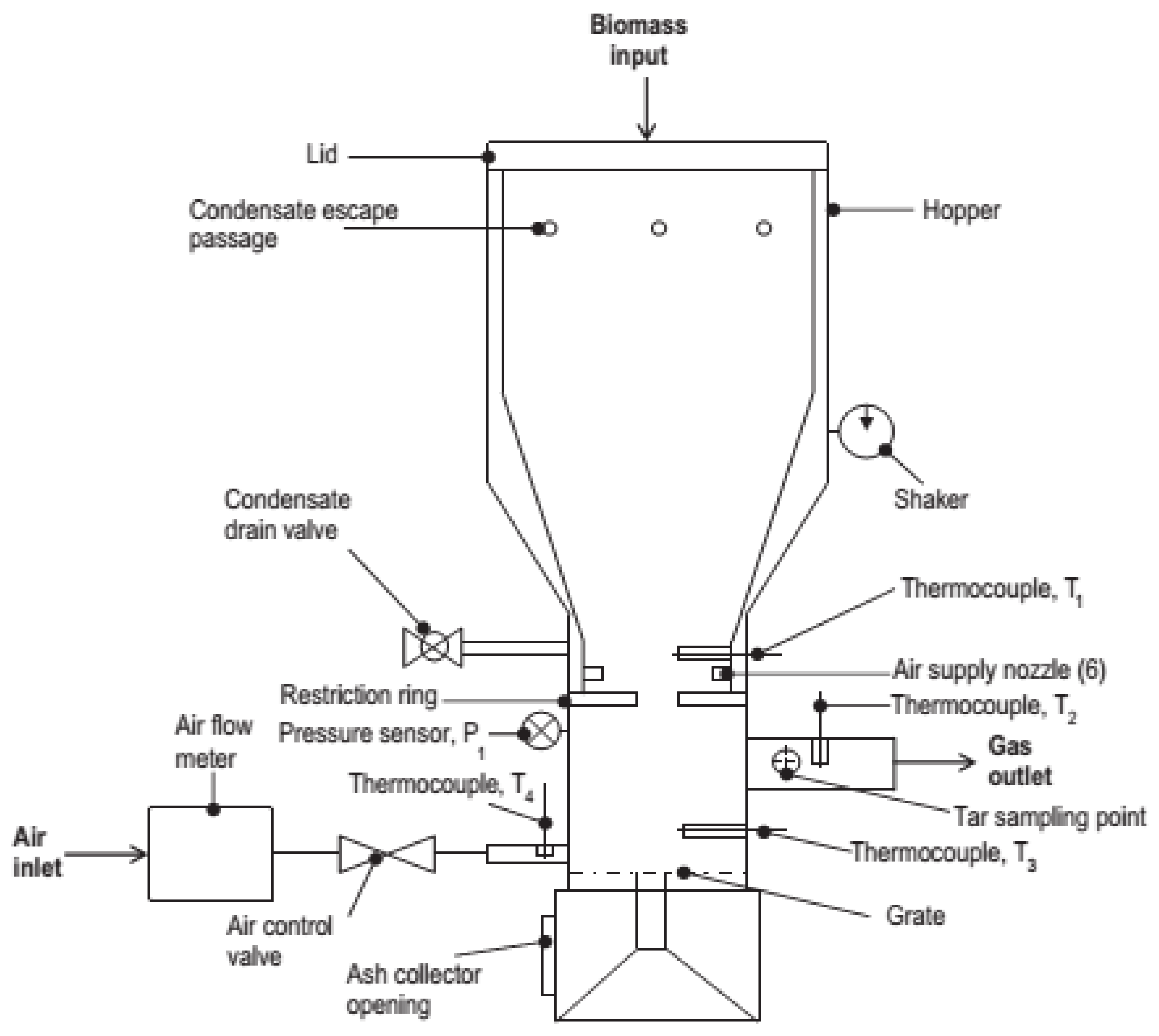
Figure 2.
Meshed gasifier geometry and customized mesh at air inlets.

Figure 3.
Mass fraction variation with time in the experimental study.
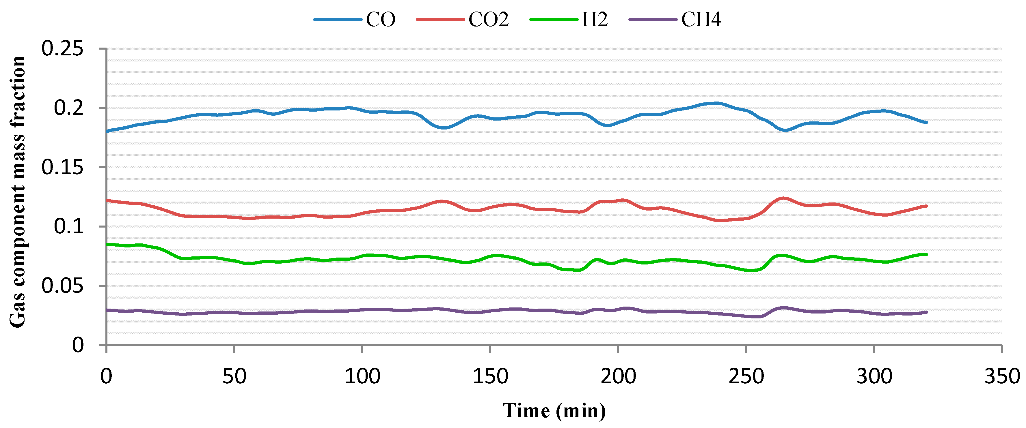
Figure 4.
Mass fraction variation with iteration in the simulation model.
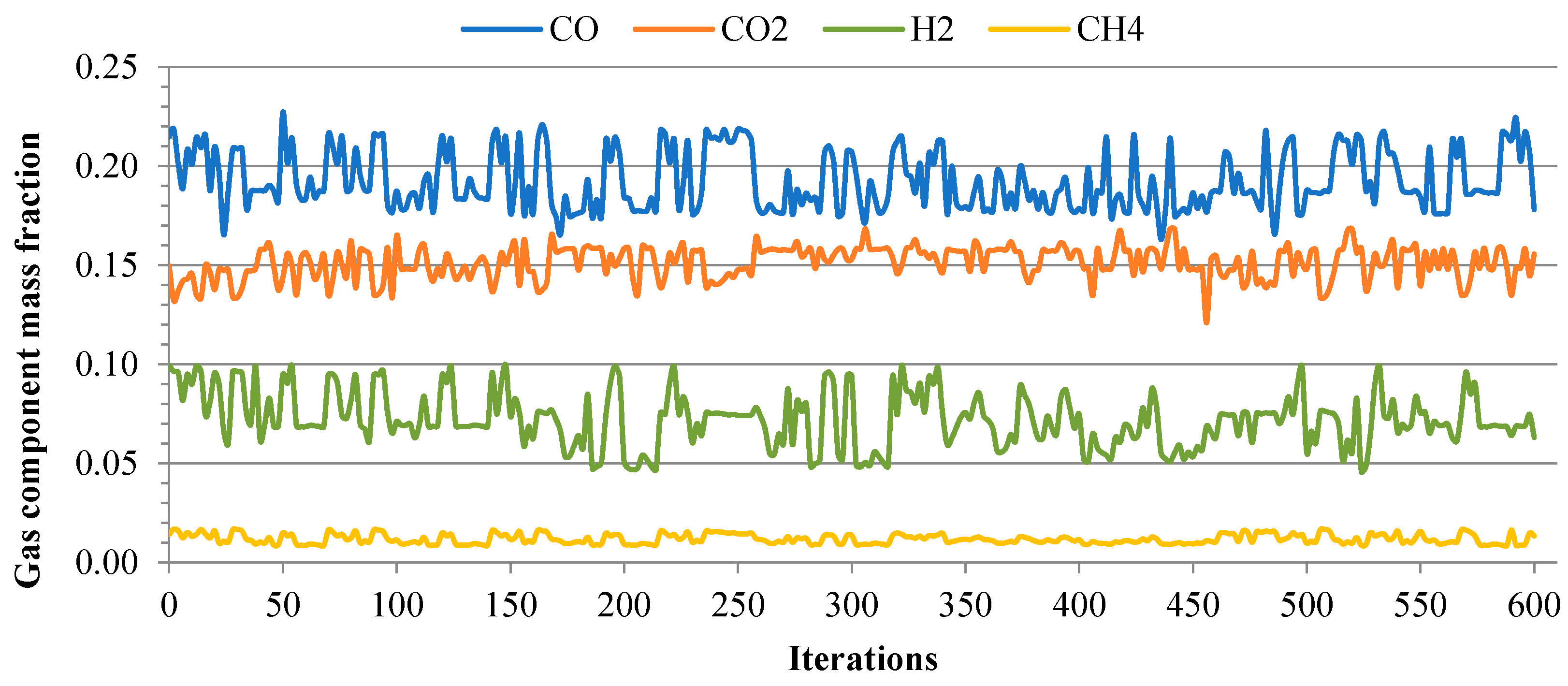
Figure 5.
Composition of the syngas predicted by model compared with experimental results.

Figure 6.
Variation of gas component mass fractions as a function of ER.

Figure 7.
Variation of Syngas yield lower heating value (LHV) and cold gas efficiency (CGE) of syngas as a function of Equivalences Ratio (ER).
Figure 7.
Variation of Syngas yield lower heating value (LHV) and cold gas efficiency (CGE) of syngas as a function of Equivalences Ratio (ER).

Figure 8.
Temperature profile inside the gasifier.
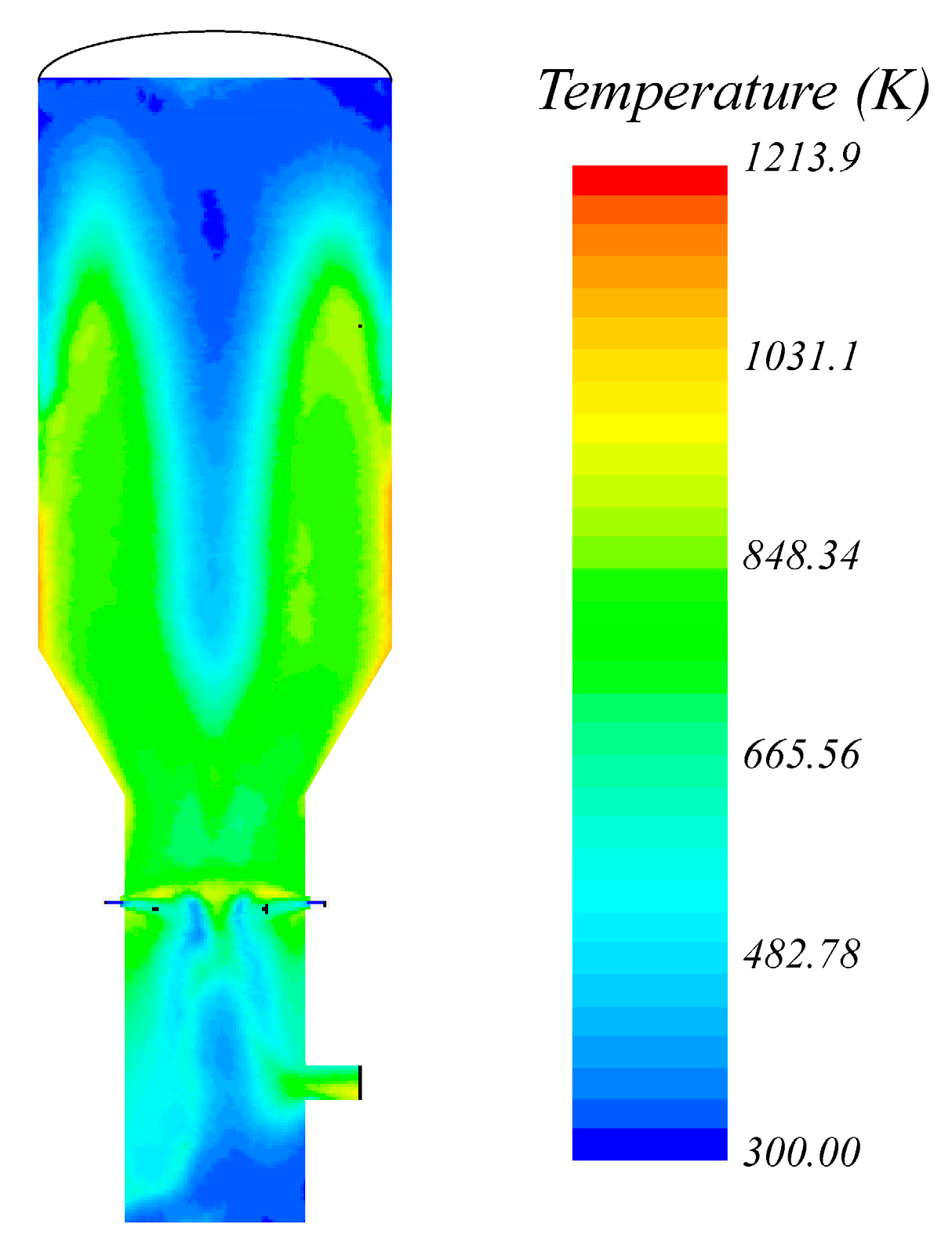
Figure 9.
Temperature variation along the mid-axis of the gasifier simulation values vs. experimental values.
Figure 9.
Temperature variation along the mid-axis of the gasifier simulation values vs. experimental values.

Table 1.
Proximate and ultimate analysis results of Birchwood [33].
Table 1.
Proximate and ultimate analysis results of Birchwood [33].
| Type of Analysis | Physical or Chemical Property | Value |
|---|---|---|
| Proximate Analysis (Dry Basis) | Moisture % | 7 |
| Volatiles % | 82.2 | |
| Fixed Carbon % | 10.45 | |
| Ash % | 0.35 | |
| LHV (MJ/kg) | 17.9 | |
| Ultimate Analysis (Dry Basis) | Carbon % | 50.4 |
| Hydrogen % | 5.6 | |
| Oxygen % | 43.4 | |
| Nitrogen % | 0.12 | |
| Sulphur % | 0.017 | |
| Chlorine % | 0.019 |
© 2017 by the authors. Licensee MDPI, Basel, Switzerland. This article is an open access article distributed under the terms and conditions of the Creative Commons Attribution (CC BY) license (http://creativecommons.org/licenses/by/4.0/).
Share and Cite
MDPI and ACS Style
Jayathilake, R.; Rudra, S. Numerical and Experimental Investigation of Equivalence Ratio (ER) and Feedstock Particle Size on Birchwood Gasification. Energies 2017, 10, 1232. https://doi.org/10.3390/en10081232
AMA Style
Jayathilake R, Rudra S. Numerical and Experimental Investigation of Equivalence Ratio (ER) and Feedstock Particle Size on Birchwood Gasification. Energies. 2017; 10(8):1232. https://doi.org/10.3390/en10081232
Chicago/Turabian StyleJayathilake, Rukshan, and Souman Rudra. 2017. "Numerical and Experimental Investigation of Equivalence Ratio (ER) and Feedstock Particle Size on Birchwood Gasification" Energies 10, no. 8: 1232. https://doi.org/10.3390/en10081232
Note that from the first issue of 2016, this journal uses article numbers instead of page numbers. See further details here.