DG Placement in Loop Distribution Network with New Voltage Stability Index and Loss Minimization Condition Based Planning Approach under Load Growth

Abstract

This paper presents a new planning approach based on voltage stability index (VSI) together with improved loss minimization (LM) formulations. The method has employed for application of distributed generation (DG) unit placement (location and size) in a loop (configured) test distribution network (LDN). Initially, VSI relationship for equivalent loop model has employed to find out potential locations for DG placement in LDN. Later, loss minimization formulations and loss minimization conditions (LMC) have been derived on the basis of an equivalent electrical model of LDN, for single and two DGs operating at various power factors, respectively. The proposed approach is comprised of two variants and has demonstrated on the 69-bus test distribution network. The first planning variant as a single case has applied for DG allocation (location, size, number) in LDN under normal load. Similarly, the second planning variant has demonstrated with three cases (six scenarios per case), evaluated under normal load and impact of load growth (across five years), respectively. The proposed approach has analyzed in terms of various performance indicators and results obtained have compared and found in close agreement with existed works in literature. Simulation results verify the validity of the proposed planning approach and establish that LDN performs better than radial distribution network from the perspective of load growth.

1. Introduction

Traditionally, distribution network (DN) in the electrical grid has been designed to retain unidirectional power flow, passive nature and operates in a radial configuration [1]. Also, increasing load demands, aging infrastructure, fewer expansion alternatives and environmental concerns are making it challenging for radial distribution network (RDN) to operate under traditional grid (TG) paradigm [2]. Moreover, competitive electricity markets and service necessities close to technical limits have resulted in serious technical issues notably; low voltage regulation over large geographic areas, high system losses, reliability issues and compromised power quality [3].

The DN on the basis of the structure has mainly been classified as radial and loop. The RDNs, despite employing simple protection schemes, are prone to aforementioned technical issues. However, in comparison, the loop distribution network (LDN) is more reliable and exhibits better voltage profile along the dedicated feeders; despite the requirements for upgraded protection schemes [4]. The multiple loop system or simply mesh distribution network (MDN) needs further advance complex protection schemes and is more prone to small values of short circuit current (SCC) level. Besides technical advantages, LDN provides a better trade-off option among radial and mesh; because of better fault traceability and reliability [4,5,6]. The RDN can be transformed into LDN by utilization of existing infrastructure, such as closing a particular (normally open) tie switch (TS), under normal operation. The loop has also advocated as a configuration of futuristic DN under smart grid (SG) environment [5]. Future or smart distribution network (SDN) has envisioned as an interconnected in nature, and intelligent from the perspective of planning and operation, respectively [6]. Hence, LDN under SG paradigm needs to be investigated as a suitable candidate for SDN.

Besides topology, distributed generation (DG) integration close to load centers has transformed passive nature of DN into an active one. As a consequence, DN modernization with various types of DGs, in planning and operation, has emerged as a prominent research dimension [7]. Several advantages have attributed to optimal DG placement (ODGP) in DN, such as [8]; system stability, reliability, loss minimizations (LM), voltage stability, load-ability enhancement, capacity release from sub-stations (SS), improvement in voltage stability margin (VSM), improved system efficiency, release of thermal loading in feeders, etc. Since RDNs were not initially designed to accommodate large penetration of DG units. Hence, DN topology based modernizations, aiming at high DG penetration (DG%) to capitalize maximum benefits, serves as a motivation for SDN planning and operations [9]. The DG accommodation (location and capacity/size) in any of the DN type makes them an active DN (ADN), where maximum achievable distribution load normally depends on static voltage limit instead of thermal limit [10].

The literature review indicates that a considerable amount of research works have been carried out aiming at various aspects (objectives) of DG placement in RDN, mainly (VSM) and LM [11]. In most of the studies, the radial structure of the DN has retained as a system constraint [3,4,11]. The DG allocation in DN has been reviewed by various researchers on the basis of size, location, types, applications, objectives, planning and solution methodologies. The most prominent classifications of solution methods include; analytical, numerical, meta-heuristics, artificial intelligence (AI), hybrid, and various miscellaneous techniques, respectively [4,11,12,13,14,15,16,17]. The voltage stability index (VSI) [11,18,19] and other loss sensitivity methods [20,21,22,23] are among the most prominent planning tools for ODGP in DN; aiming at achieving multiple conflicting nature objectives, respectively. Murthy et al. [24] presents a noticeable work addressing MDN, aiming at sensitivity based approach for LM with ODGP. Alvarez-Herault et al. [25] have presented a comparative study of four methods, targeting high DG penetration in MDN; by replacing normally open TS with quick deloopers based on fault current limiter devices, as an expensive alternative, respectively. Furthermore, simultaneous VM and LM attainment in DN with multiple DG units is a prominent research dimension as advocated in [26,27].

Numerous VSI based numerical methods have been proposed in the literature for optimal DG location and size, based on the equivalent two-bus model, for improving VSM of RDNs, respectively [28,29,30,31,32]. The VSIs have employed in previous studies to find candidate DG location in RDN for simultaneous voltage maximization (VM) and system LM, respectively [18,19,26,27,28,29,30,31,32]. Also, the VSI based planning problems for ODGP under load growth across a planning horizon, are mostly limited to RDNs [30,31,32,33]. However, limited works have available in the literature that utilized VSI specifically proposed for LDN, to access LM and VM; with ODGP. A significant interest has appreciated in arraying closed-loop configured DN for SG and favored from the viewpoint of better voltage stability, DG penetration, reliability and achievable fault traceability [4,5,34,35,36]. Since an ADN as SDN is expected to operate in loop topology [6] and VSIs for RDN are not applicable for the desired application. In addition, it is advocated in [23,37] that the voltage magnitude only is not an appropriate indicator for accessing voltage stability of a DN. Thus, a more flexible VSI proposed in [36] is employed, to address voltage stability assessment of LDN. Besides, VSI in [36] is capable of considering bidirectional power flow feeding a receiving end (load bus) from two sending ends. Furthermore, none of the aforementioned works have utilized VSI for ODGP, specifically proposed for LDN; aim at simultaneously achieving LM and VM simultaneously, under load growth across planning horizons, respectively. The bridging of research gaps serves the motivation of this paper.

In this paper, the proposed planning approach consists of VSI in [36] together with improved LM formulations, which have utilized for the application of DG placement (location and capacity) in a test LDN. The planning approach consists of two variants and applied for aimed objectives, which includes improving DG%, VM, LM, associated performance indicators and planning from the perspective of future load growth, respectively. The key contributions of this work are as follows.

(1)

DG allocation in LDN with a new VSI based approach.

(2)

Derivation of formulations for LM; based on equivalent electrical models of LDN.

(3)

Evaluation of loss minimization condition (LMC) in LDN with single and two DGs under various power factors (PF); such as unity PF (PF1) and lagging PF (PFL), respectively.

(4)

Demonstration of planning approach (comprised of two variants) on 69-bus test DN.

(5)

Demonstration of DG allocation in LDN as first variant of planning approach for LM and VM.

(6)

Demonstration of three cases (variant 2) with various scenarios for one and two DG placement.

(7)

Evaluations of DGP under load growth scenarios.

(8)

Detail comparison of single and two DG placement on various performance indicators.

(9)

Overall comparison of results with other methods available in the literature.

The remaining paper is organized as follows. Section 2 presents an overview of background concepts, mainly VSI and circuit equivalent model based formulations for LM in LDN, respectively. Section 3 examines the proposed planning approach (variant 1) for simultaneously achieve LM and VM, using DG units, respectively. Section 4 offers results, evaluation, and discussion regarding variant 2 of the proposed approach. The overall performance analysis and comparison with existing research works have presented in Section 5. The paper is concluded in Section 6.

2. Background Concepts

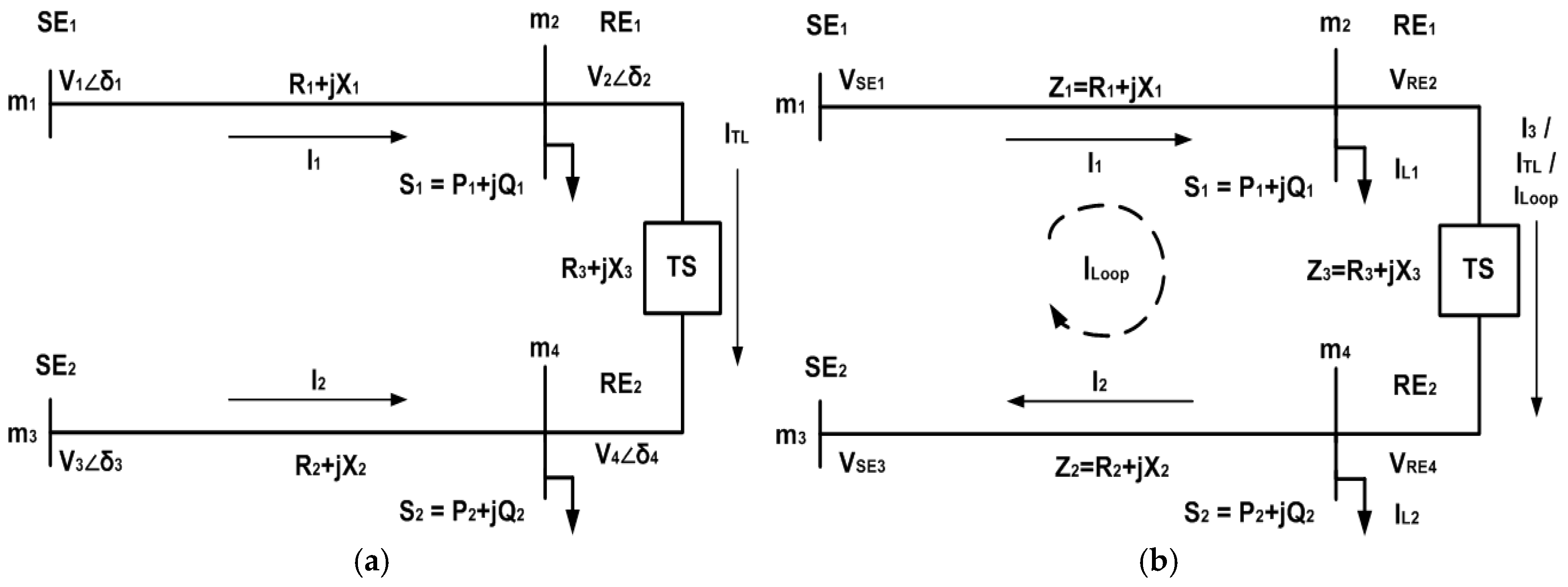
2.1. Voltage Assesment Method for Loop Distribution Network

This paper utilizes VSI for LDN, derived in [36], and based on circuit analysis and bi-quadratic methods; to offer a simple planning approach for DGP under normal load and load growth impact, respectively. The objectives are to simultaneously achieve LM, VM, increase DG penetration (DG%), and associated benefits in LDN planning, respectively. Figure 1a illustrates a simple electrical equivalent loop model for the VSI evaluation of LDN [36] and is similar to one line diagrams based on three distribution lines as considered in [4,5]. The type I loop, being simple and feasible, is considered for a study where two radial feeders form a closed loop and is fed by the same power transformer [5,36]. The relevant detail regarding VSI for LDN can be found in [36]. The expression for VSI and receiving end voltage (V_R or V₂), derived for real case including parameters of tie-line (TL) and tie-switch (TS); are shown in Equations (1) and (2) as follows, respectively.

$$\begin{array}{c}{\mathrm{VSI}\left({\mathrm{m}}_2\right)}_{\mathrm{LDN}}={\sum }_{i=1}^{n_l}{\left[\frac{\left|V_{nse}\right|}{n_l}\right]}^4-2{\sum }_{i=1}^{n_l}{\left[\frac{\left|V_{nse}\right|}{n_l}\right]}^2\left[\left[\frac{A}{(R_1+\Delta R)}\right]+\left[\frac{B}{(X_1+\Delta X)}\right]\right]-\\ {\left[\frac{A}{(R_1+\Delta R)}-\frac{B}{(X_1+\Delta X)}\right]}^2\ge 0\end{array}$$

(1)

where, V_nse are the voltages of sending end (SE) nodes, n_l is the number of SE nodes feeding receiving end (RE) node in a LDN, A = p₂ (R₁R₃ − X₁X₃) + Q₂ (R₁X₃ + R₃X₁) and B = p₂ (R₁X₃ + R₃X₁) − Q₂ (R₁R₃ − X₁X₃). [Z₁ + ΔZ] is a common term, |ΔZ| = |Z₁ − Z₃| ≥ 0 for open branches in the loop and |ΔZ| = Z₃ for TL, feeding RE node m₄ from another SE node (m₂), respectively. The RE node voltage (V_R) in term of the real root; i.e., VSI (as determinant) in Equation (1), is presented in Equation (2) as a feasible solution, respectively.

$$\left|V_R\right|=0.707\sqrt{\left[{\displaystyle {\displaystyle \sum }_{l=1}^{n_l}}{\left[\frac{\left|V_{nse}\right|}{n_l}\right]}^2-\left[\frac{A}{(R_1+\Delta R)}\right]+\left[\frac{B}{(X_1+\Delta X)}\right]\right]+\sqrt{\begin{array}{c}{\displaystyle {\displaystyle \sum }_{l=1}^{n_l}}{\left[\frac{\left|V_{nse}\right|}{n_l}\right]}^4-2{\displaystyle {\displaystyle \sum }_{l=1}^{n_l}}{\left[\frac{\left|V_{nse}\right|}{n_l}\right]}^2\left[\left(\frac{A}{(R_1+\Delta R)}\right)+\left(\frac{B}{(X_1+\Delta X)}\right)\right]\\ -1{\left[\frac{A}{(R_1+\Delta R)}-\frac{B}{(X_1+\Delta X)}\right]}^2\end{array}}}$$

(2)

2.2. Loss Minimization Formulations in Loop Distribution Network

The LM formulations in LDN has represented with modified electrical equivalent model of LDN, as shown in Figure 1b, which consists of three distribution lines. The research work in [4] provides the basis for derived formulations. Besides feeders 1 and 2, line 3 represents TL, which links the two feeders (1 and 2) in loop configuration [4]. The LM formulations have represented with three cases, first is without DG. The second case aims at LMC in LDN with one DG and the third case aims at LMC with two DGs placement, at PF1 (generates active power only) and PFL (generates both active and reactive power), respectively.

2.2.1. Loss Minimization Case without Distributed Generation Units in Loop Distribution Network

The feeder currents in closed loop are shown as $I_{CL}^{F1}=I_1+I_3,I_{CL}^{F2}=I_1-I_3$ and $\left|I_{CL}^{TL}\right|=|(V_2-V_4)/(R_3+j{X}_3)|$ for feeder 1, 2 and TL, respectively. When the configuration of test DN has changed to loop, the current of the light loaded feeder increases as TL current (I_TL) and heavy loaded feeder has reduced by same amount of I_TL [4].

The impedance of each line has represented with Z_j = R_j + jX_j (where j = 1, 2, 3), where the line resistance is shown with R_j and line reactance with X_j; respectively. Since, the loop system has fed from two sources, hence two sending (V_SE1 and V_SE3) and receiving end (V_RE2 and V_RE4) voltages have considered in the modified model to completely cover all the aspects of an actual LDN. The loads at receiving ends have considered as constant current/power source in this derivation. In addition, node m₂ has considered lightly loaded than node m₄, i.e., the loop current flows across the TL from m₂ to m₄. On the basis of line currents in LDN model, the power flow can be formulated on the basis of superposition principle, shown in Equations (3a) and (3b), respectively; as follows [4].

$$\begin{gathered} I_1=\left(Z_2+Z_3\right)I_{L1}+Z_2{I}_{L2}+\left(V_{SE1}-V_{SE3}\right)/Z_{Loop} \\ {I}_2=-\left(Z_1+Z_3\right)I_{L2}-Z_1{I}_{L1}+\left(V_{SE1}-V_{SE3}\right)/Z_{Loop} \\ {I}_3=I_{TL}=-Z_1{I}_{L1}+Z_2{I}_{L2}+\left(V_{SE1}-V_{SE3}\right)/Z_{Loop} \end{gathered}$$

(3a)

$$Z_{Loop}={\displaystyle {\displaystyle \sum }_{j=1}^3}{Z}_j;R_{Loop}={\displaystyle {\displaystyle \sum }_{j=1}^3}{R}_j;X_{Loop}={\displaystyle {\displaystyle \sum }_{j=1}^3}{X}_j$$

(3b)

The total power losses (TPL) in LDN can be formulated as follows:

$$\begin{array}{c}{P}_{Loss\_Total}^{CL}={\displaystyle {\displaystyle \sum }_{i=1}^{na}}{\left|I_1\right|}^2{Z}_1+{\displaystyle {\displaystyle \sum }_{i=1}^{nb}}{\left|I_2\right|}^2{Z}_2+{\displaystyle {\displaystyle \sum }_{t=1}^{nt}}{\left|I_3\right|}^2\left(Z_{Loop}\right)\\ +2\left({\displaystyle {\displaystyle \sum }_{t=1}^{nt}}\left|I_{CL}^{F1}\right|Z_1-\left|I_{CL}^{F2}\right|Z_2\right)\left|I_3\right|\end{array}$$

(4)

The Equation (4) can be rearranged in Equation (5) as follows:

$$\begin{array}{c}{P}_{Loss\_Total}^{CL}={\displaystyle {\displaystyle \sum }_{i=1}^{na}}{\left|I_{CL}^{F1}\right|}^2{Z}_1+{\displaystyle {\displaystyle \sum }_{i=1}^{nb}}{\left|I_{CL}^{F1}\right|}^2{Z}_2+{\displaystyle {\displaystyle \sum }_{t=1}^{nt}}{\left|I_{CL}^{F1}\right|}^2\left(Z_1+Z_2+Z_3\right)\\ +2\left({\displaystyle {\displaystyle \sum }_{t=1}^{nt}}\left|I_{CL}^{F1}\right|Z_1-\left|I_{CL}^{F2}\right|Z_2\right)\left|I_{CL}^{F1}\right|\end{array}$$

(5)

On the basis of line loss minimization theory aiming at LDN, as indicated in [4], the line currents can be distinctly divided among; currents flowing through lines/branches and through tie-lines as loop currents; respectively. Thus, total active losses (TPL) and reactive (TQL) power losses in LDN can be formulated as shown in Equations (6a) and (6b); respectively.

$$\begin{array}{c}{TPL}_{Loss\_Total}^{CL}={\displaystyle {\displaystyle \sum }_{i=1}^{na}}{\left|I_1\right|}^2{R}_1+{\displaystyle {\displaystyle \sum }_{i=1}^{nb}}{\left|I_2\right|}^2{R}_2+{\displaystyle {\displaystyle \sum }_{t=1}^{nt}}{\left|I_3\right|}^2\left(R_{Loop}\right)\\ +2\left({\displaystyle {\displaystyle \sum }_{t=1}^{nt}}\left|I_{CL}^{F1}\right|R_1-\left|I_{CL}^{F2}\right|R_2\right)\left|I_3\right|\end{array}$$

(6a)

$$\begin{array}{c}{TQL}_{Loss\_Total}^{CL}={\displaystyle {\displaystyle \sum }_{i=1}^{na}}{\left|I_1\right|}^2{X}_1+{\displaystyle {\displaystyle \sum }_{i=1}^{nb}}{\left|I_2\right|}^2{X}_2+{\displaystyle {\displaystyle \sum }_{t=1}^{nt}}{\left|I_3\right|}^2\left(X_{Loop}\right)\\ +2\left({\displaystyle {\displaystyle \sum }_{t=1}^{nt}}\left|I_{CL}^{F1}\right|X_1-\left|I_{CL}^{F2}\right|X_2\right)\left|I_3\right|\end{array}$$

(6b)

If the loop current (I_Loop or I₃) has eliminated, maximum LMC can be achieved and the modified expressions can be re-written as shown in Equations (7a) and (7b), respectively. Also, it can be safely concluded that besides sending end voltages (V_SE1 and V_SE3), the potential difference between V_RE2 and V_RE4 needs to be ideally zero, to satisfy maximum LMC.

$${TPL}_{Loss\_min}^{CL}={\displaystyle {\displaystyle \sum }_{i=1}^{na}}{\left|I_1\right|}^2{R}_1+{\displaystyle {\displaystyle \sum }_{i=1}^{nb}}{\left|I_2\right|}^2{R}_2$$

(7a)

$${TQL}_{Loss\_min}^{CL}={\displaystyle {\displaystyle \sum }_{i=1}^{na}}{\left|I_1\right|}^2{X}_1+{\displaystyle {\displaystyle \sum }_{i=1}^{nb}}{\left|I_2\right|}^2{X}_2$$

(7b)

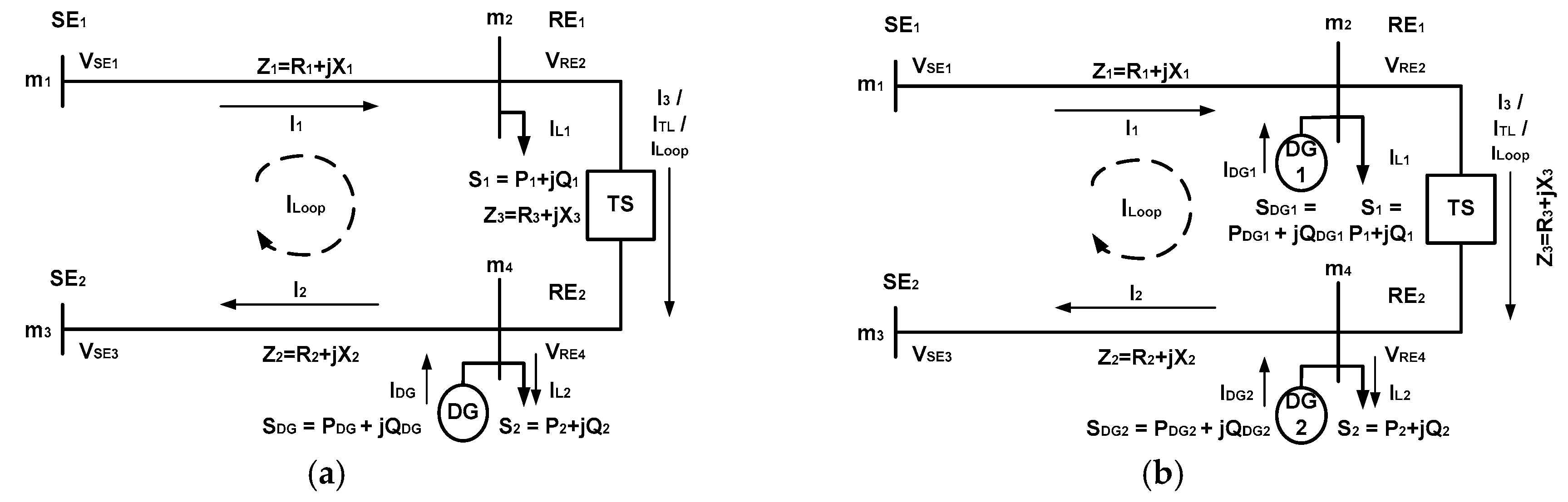
2.2.2. Loss Minimization Case with One Distributed Generation Unit in Loop Distribution Network

The main aim, in this case, is to illustrate the impact on one DG in achieving LMC, as shown in Figure 2a. The DG (with associated power and current) has assumed to acts as a negative load and the direction of current is opposite to the load current I_L2. The general modified expressions for currents in lines and loops; can be formulated as shown in Equation (8).

$$\begin{gathered} {I_1}^{1DG}=\left(Z_2+Z_3\right)I_{L1}+Z_2(I_{L2}-I_{DG})+\left(V_{SE1}-V_{SE3}\right)/Z_{Loop} \\ {I_2}^{1DG}=-\left(Z_1+Z_3\right)(I_{L2}-I_{DG})-Z_1{I}_{L1}+\left(V_{SE1}-V_{SE3}\right)/Z_{Loop} \\ {I}_{TL}={I_3}^{1DG}=-Z_1{I}_{L1}+Z_2(I_{L2}-I_{DG})+\left(V_{SE1}-V_{SE3}\right)/Z_{Loop} \end{gathered}$$

(8)

The optimal value of DG current (I_DG) and relevant capacity can result in significant minimization of the TL current (I_TL) in particular and overall loop current as a whole. Hence, a noteworthy LMC can be attained. It is worth mentioning that optimal DG capacity with a respective value of I_DG must result in an increase of V_RE4 at heavy loaded node m₄ i.e., the potential difference across node m₂ and m₄ is ideally zero. The modified overall LM expressions for TPL and TQL can be rearranged, as in Equations (9a) and (9b); as follows:

$${TPL}_{LM\_1DG}^{CL}={\displaystyle {\displaystyle \sum }_{i=1}^{na}}{\left|{I_1}^{1DG}\right|}^2{R}_1+{\displaystyle {\displaystyle \sum }_{i=1}^{nb}}{\left|{I_2}^{1DG}\right|}^2{R}_2$$

(9a)

$${TQL}_{LM\_1DG}^{CL}={\displaystyle {\displaystyle \sum }_{i=1}^{na}}{\left|{I_1}^{1DG}\right|}^2{X}_1+{\displaystyle {\displaystyle \sum }_{i=1}^{nb}}{\left|{I_2}^{1DG}\right|}^2{X}_2$$

(9b)

2.2.3. Loss Minimization Case with Two Distributed Generation Units in Loop Distribution Network

A significant minimization of the system losses can be achieved by optimal placement of two DGs in LDN, as shown in Figure 2b. The optimal value of first DG indicated as DG1 in Figure 2b with current I_DG1 and DG2 with current I_DG2 can result in reducing I_TL in particular and overall loop current as a whole, respectively. The DG1 has placed at node m₂ with light load density, whereas DG2 has placed at node m₄ with high load density, respectively.

It can be safely suggested that besides sending end voltages (V_SE1 and V_SE3), the two DG placement with optimal capacity and current values (I_DG1 and I_DG2), can results in an optimal reduction of potential difference among V_RE2 and V_RE4, aiming at minimizing I_TL and seems promising to satisfy maximum LMC. The modified expressions for currents in lines and loops, after placement of two DGs; can be formulated as shown in Equation (10).

$$\begin{gathered} {I_1}^{2DG}=[\left(Z_2+Z_3\right)\left(I_{L1}-I_{DG1}\right)+Z_2(I_{L2}-I_{DG2})+\left(V_{SE1}-V_{SE3}\right)]/Z_{Loop} \\ {I_2}^{2DG}=\left[-\left(Z_1+Z_3\right)(I_{L2}-I_{DG2}\right)-Z_1\left(I_{L1}-I_{DG1}\right)+\left(V_{SE1}-V_{SE3}\right)]/Z_{Loop} \\ {I_3}^{2DG}=\left[-Z_1\left(I_{L1}-I_{DG1}\right)+Z_2(I_{L2}-I_{DG2}\right)+\left(V_{SE1}-V_{SE3}\right)]/Z_{Loop} \end{gathered}$$

(10)

The modified LMC expressions for total active and reactive power losses, aiming at two DG units placement in LDN, can be reformulated as shown in Equations (11a) and (11b); as follows:

$${TPL}_{LM\_2DG}^{CL}={\displaystyle {\displaystyle \sum }_{i=1}^{na}}{\left|{I_1}^{2DG}\right|}^2{R}_1+{\displaystyle {\displaystyle \sum }_{i=1}^{nb}}{\left|{I_2}^{2DG}\right|}^2{R}_2$$

(11a)

$${TQL}_{LM\_2DG}^{CL}={\displaystyle {\displaystyle \sum }_{i=1}^{na}}{\left|{I_1}^{2DG}\right|}^2{X}_1+{\displaystyle {\displaystyle \sum }_{i=1}^{nb}}{\left|{I_2}^{2DG}\right|}^2{X}_2$$

(11b)

2.2.4. Impact of Distributed Generation Units Operating at Various Power Factors on Loss Minimization

In this subsection, the impact of DG’s PFs on LM has briefly illustrated. Since type-I DGs operating at PF1 are capable of injecting active power only. Hence, the active component of DG current (I_aDG) injects at the respective nodes of DG placement and more active power minimization is noticeable. To illustrate PF impact of DG, LM case with two DGs has considered. The modified expressions for the impact of the active component of DG currents in lines and loops, after placement of two DGs at PF1; can be formulated as active and reactive components; as shown in Equations (12a) and (12b), respectively.

$$\begin{gathered} {I_{a1\_PF1}}^{2DG}=\left[\left(R_2+R_3\right)\left(I_{L1}-I_{aDG1}\right)+R_2(I_{L2}-I_{aDG2})+\left(V_{SE1}-V_{SE3}\right)\right]/R_{Loop} \\ {I_{a2\_PF1}}^{2DG}=\left[-\left(R_1+R_3\right)(I_{L2}-I_{aDG2})-R_1\left(I_{L1}-I_{aDG1}\right)+\left(V_{SE1}-V_{SE3}\right)\right]/R_{Loop} \\ {I_{a3\_PF1}}^{2DG}=\left[-R_1\left(I_{L1}-I_{aDG1}\right)+R_2(I_{L2}-I_{aDG2})+\left(V_{SE1}-V_{SE3}\right)\right]/R_{Loop} \end{gathered}$$

(12a)

$$\begin{gathered} {I_{r1\_PF1}}^{2DG}=\left(X_2+X_3\right)I_{L1}+X_2{I}_{L2}+\left(V_{SE1}-V_{SE3}\right)/X_{Loop} \\ {I_{r2\_PF1}}^{2DG}=-\left(X_1+X_3\right)I_{L2}-X_1{I}_{L1}+\left(V_{SE1}-V_{SE3}\right)/X_{Loop} \\ {I_{r3\_PF1}}^{2DG}=-X_1{I}_{L1}+X_2{I}_{L2}+\left(V_{SE1}-V_{SE3}\right)/X_{Loop} \end{gathered}$$

(12b)

The DGs that operate at PFL are capable to inject both active and reactive powers. The active component of DG current (I_aDG) and reactive counterpart (I_rDG); injected at the respective nodes of DG placement tends to achieve both active and reactive power losses by a high percentage. The highest LM can be attained if DGs have same PF as that of system load in test DN. The modified expressions for the impact of an active and reactive component of DG currents in lines and loops, after placement of two DGs at PFL; can be formulated as active and reactive components; as shown in Equations (13a) and (13b), respectively.

$$\begin{gathered} {I_{a1\_PFL}}^{2DG}=\left[\left(R_2+R_3\right)\left(I_{L1}-I_{aDG1}\right)+R_2(I_{L2}-I_{aDG2})+\left(V_{SE1}-V_{SE3}\right)\right]/R_{Loop} \\ {I_{a2\_PFL}}^{2DG}=\left[-\left(R_1+R_3\right)(I_{L2}-I_{aDG2})-R_1\left(I_{L1}-I_{aDG1}\right)+\left(V_{SE1}-V_{SE3}\right)\right]/R_{Loop} \\ {I_{a3\_PFL}}^{2DG}=\left[-R_1\left(I_{L1}-I_{aDG1}\right)+R_2(I_{L2}-I_{aDG2})+\left(V_{SE1}-V_{SE3}\right)\right]/R_{Loop} \end{gathered}$$

(13a)

$$\begin{gathered} {I_{r1\_PFL}}^{2DG}=\left[\left(X_2+X_3\right)\left(I_{L1}-I_{rDG1}\right)+X_2(I_{L2}-I_{rDG2})+\left(V_{SE1}-V_{SE3}\right)\right]/X_{Loop} \\ {I_{r2\_PFL}}^{2DG}=\left[-\left(X_1+X_3\right)(I_{L2}-I_{rDG2})-X_1\left(I_{L1}-I_{rDG1}\right)+\left(V_{SE1}-V_{SE3}\right)\right]/X_{Loop} \\ {I_{r3\_PFL}}^{2DG}=\left[-X_1\left(I_{L1}-I_{rDG1}\right)+X_2(I_{L2}-I_{rDG2})+\left(V_{SE1}-V_{SE3}\right)\right]/X_{Loop} \end{gathered}$$

(13b)

2.3. Distributed Generation Penetration by Percentage in Loop Distribution Network

DG penetration (DG%) level in percentage (%) is the ratio of total power generated by k DGs (P_DG) over total load across n nodes (P_LD) in a DN (except a slack bus) [34]; is shown in Equation (14):

$$\mathrm{DG}\%=\left({\displaystyle {\displaystyle \sum }_{i=1}^k}{P}_{DG}/{\displaystyle {\displaystyle \sum }_{j=1}^n}{P}_{LD}\right)\times 100$$

(14)

2.4. Cost of Energy Losses in Loop Distribution Network

The rate of electricity (E_c) is considered 0.06 $/KWh and time duration (T) is in a year (8760 h). The fundamental evaluation paradigm is the cost of energy loss, which is the annual cost of energy loss (CEL) or active power loss (CPL) and presented by Equation (15) as follows [32]:

$$\mathrm{CEL}=\left[TotalRealpowerlossor\left(\mathrm{TPL}\right)\right]\times \left[E_c\times T\left(year\right)\right]$$

(15)

2.5. Annual (Annualized) Investment Cost of Distributed Generation Units

The annual or annualized investment cost (AIC) of DG units has normally considered in proportional relationship with maximum DG capacity (DGC). The cost of DG unit varies for different associated types, on the basis of their nature and PF equal to that of DN, respectively. The amount of investment cost (IC) has transformed to annualized cost in the start of planning period by utilizing annualized factor (${AF}_k$). The parameters in the evaluation of AIC have shown in

Table 1. Parameter in the evaluation of AIC [34].

Description	Simulation Parameters
DG Technology	Photovoltaic (PV)	Gas-Turbine
DG Type (T) by PF	PF = 1/Type-I (T-I)	Lag/Type-II (T-II)
DGCmax (MVA)/(MW)	0.001 to 4	0.001 to 4
CUk (USD/KVA)	5250	1800
Life Span (Years)	20	10
Interest Rate (IR%)	7%	7%

. The relationship of AIC and AF_k has shown in Equations (16a) and (16b), respectively, as follows [34]:

$$\mathrm{AIC}\left(Million\frac{USD}{Year}\right)={\displaystyle {\displaystyle \sum }_{k=1}^{N_{DG}}}{AF}_k\times {CU}_k\times {\mathrm{DGC}}_{\max }$$

(16a)

$${AF}_k=\frac{\left(\frac{k}{100}\right){\left(1+\frac{k}{100}\right)}^t}{{\left(1+\frac{k}{100}\right)}^t-1}$$

(16b)

where, ${AF}_k$ is the annualized factor, ${CU}_k$ is the cost of DG unit in USD/KVA, DGC_max is the maximum capacity of DG, k is the annual cost based on certain interest rate (IR) by %, which is normally 7% and t = service life of DG (a parameter in evaluation of life cycle cost); respectively [34].

3. Proposed Planning Approach

The power utilities have obligation to retain load voltage profiles on distribution feeders near rated value under all situations. Load imbalances among feeders increase losses in distribution networks. The proposed approach has applied to find out various major objectives pertaining to planning, in particular; voltage stability and LM, for the efficient operation of a DN.

The proposed approach has applied to 69-bus test distribution system, as shown in Figure 3 with loop configuration, aiming at potential locations for DG locations. The main objectives include retaining suitable voltage profile, minimize system losses, eliminate load imbalance among feeders in the loop and attain high DG penetration. The total real and reactive power loads of 69-bus test system consists of 3802.6 KW and 2692.7 KVAR, respectively.

The total system losses in the radial topology without DG account for 224.96 KW (TPL) of active and 102.1096 KVAR (TQL) of the reactive component, respectively. The test LDN model includes seven feeders/laterals and five tie-switches. The TS5 is closed for to make loop 5 in LDN in this study, as explained in [36] comprehensively. Loop 5 is the weakest loop on the basis of VSI in [36] and indicates the weakest node as a potential location for DGP.

The proposed planning approach has applied in two variants. In the first variant, potential DG locations, size, and quantity are found to simultaneously achieve LM and VM in LDN, under normal load, respectively. In the second variant, three cases for LM, VM and both (simultaneous LM and VM) have studied; with one and two DGs placements; considering (besides normal load) the impact of load growth across five years, respectively. The discussion on the analysis of results aiming at intermediate planning years is avoided, for retaining the notion of the study precise and to the point, respectively. In addition, assumptions in proposed approach in Appendix A, simulator details in Appendix B and specifications (and simulation conditions) of 69-bus test DN in Appendix C, have shown separately at the end of the paper; respectively.

3.1. Variant 1: Potential Locations for Distributed Generation Units in Loop Distribution Network

The VSI evaluation for actual case (based on equivalent loop model) being a realistic approach has been demonstrated for initially finding potential locations for DGP in LDN under normal load (3802.6 KW and 2692.7 KVAR), and indicated as variant 1 (or case 0) of proposed planning approach. The outline of variant 1 for optimal DG location, aim at simultaneously LM and VM, is shown as follows:

(1)

Find potential locations for DG allocation in test LDN.

(2)

Considers DGP at PF1 and PFL equal to PF of test LDN, respectively.

(3)

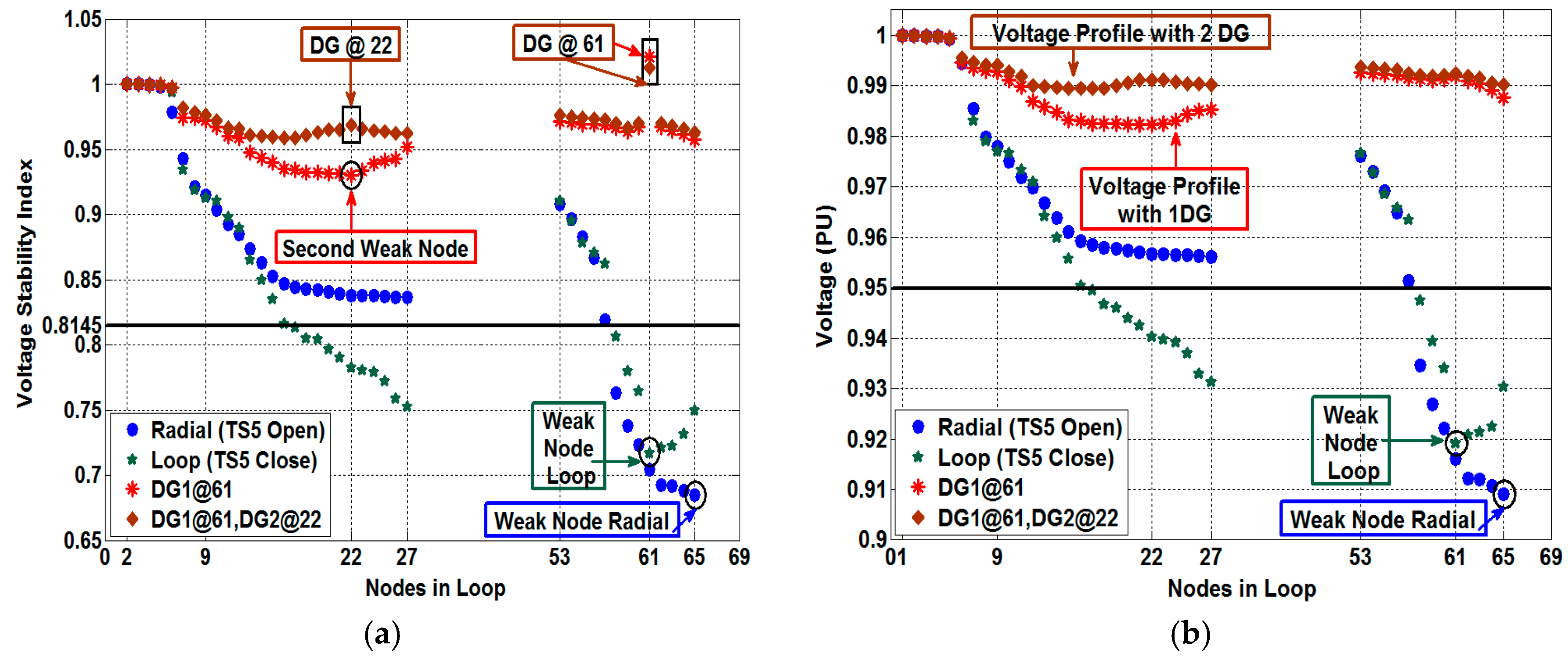
The impacts of DGP have shown in terms of proposed VSI values and associated voltage profile; respectively.

The computation procedure for variant 1, applied on 69-bus test DN, is shown as follows:

Step 1

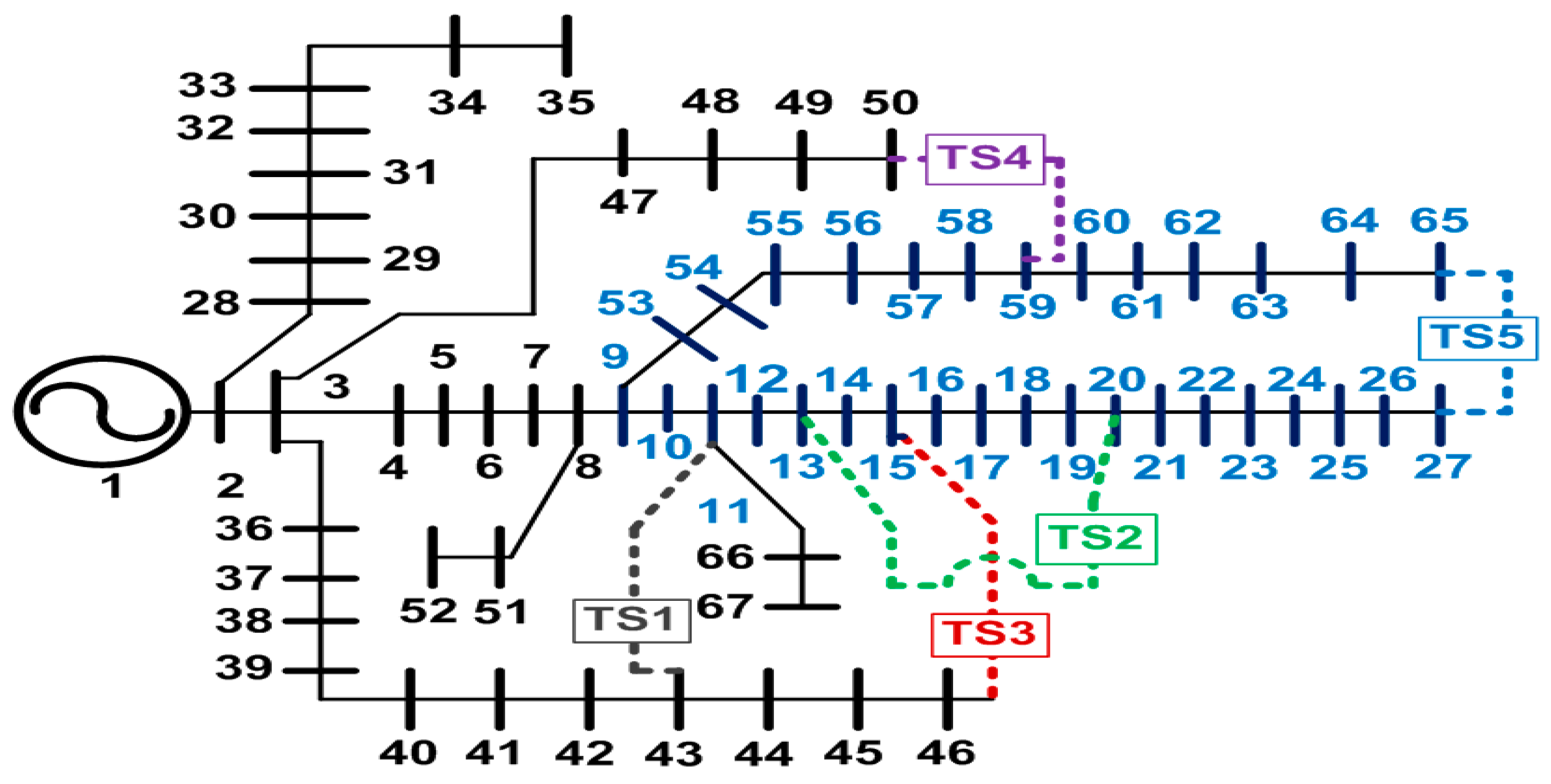
Read system data and select the potential tie-switch (TS) for the loop case, as in [36].

Step 2

Run the power flow for test LDN without DG at normal load level (CP-SLL).

Step 3

Calculate proposed VSI and receiving end node voltage (V_R) value, for real case at each node in the loop in accordance with Equations (1) and (2), respectively, as derived in [36].

Step 4

Select the node with minimum VSI value, since this node is potential candidate for first DG (DG1) placement.

Step 5

Run power flow for test LDN with DG1 at normal load level. Increase capacity of DG1 at lagging power factor ± 2% (or unity power factor), which is equal to the power factor of DN load (0.82 ± 2%). The PFL is taken 0.82 ± 2% as a reference to cater small load variations.

Step 6

Calculate proposed VSI for real case at DG node in LDN according to Equation (1) i.e., resulting voltage at node with DG as in Equation (2); approaches a numerical value close to 1.0 pu, that is nearly equal or little less than substation reference voltage; respectively.

Step 7

Select the node with minimum VSI value after DG1 installation, since this new node is the potential candidate for second DG (DG2) placement.

Step 8

Repeat step 5 i.e., the power flow across the TL and I_TL must be ideally zero, such that the VSI and V_R values of end nodes across TL (including TS) have a minimum difference of numerical values, according to Equations (1) and (2), respectively.

Step 9

Furthermore, increase and decrease the capacities of DG2 and DG1 (at PF1 or PFL = 0.82 ± 2%) in steps; and find out the LMC according to Equations (11a) and (11b), respectively.

Step 10

When the end-nodes across the TL (including TS) have the lowest difference of the numerical values according to Equations (1), (2), (11a) and (11b); the condition for VM and LMC has met, i.e., respective DG capacities and their power factors (PF) are optimal choices.

3.1.1. Discussion on Results with Type-II Distributed Generation Units in Loop Distribution Network

On the basis of the proposed planning approach, potential locations for DG placement in test LDN aims at; voltage stability improvement, system loss minimizations, and other associated objectives. Two types of DG units have considered here. First, DG with PFL (nearly equal to the PF of LDN) has considered (also shown as type-II) and is capable of injecting both active and reactive powers. The second type of DG unit operating at PF1 is type-I that is capable of injecting active power only. Figure 4a,b show evaluations of proposed approach, applied on 69-bus test DN; in terms of VSI Equation (1) and voltage profile Equation (2) values, after installing type-II DG at PFL, respectively. During Steps 1–4, loop 5 (by closing TS5 between nodes 27 and 65) indicates the potential candidate to demonstrate the application of proposed approach as per [36]. The weakest node in the radial configuration without DG is 65 (VSI = 0.6845 and V = 0.909 pu) as given in [28], whereas in loop configuration that is 61(VSI = 0.7172 and V = 0.92 pu) [36]. According to step 5, place first DG (DG1) at node 61 in test LDN and increase the capacity at an optimal power factor equal to DN load (0.82 ± 2%) i.e., the node voltage approaches close to reference sub-station (SS) voltage, that is 1.0 pu.

In step 6, the corresponding values of VSI and voltage for PFL based DG at node 61; are 1.0207 and 0.992 pu, respectively. The DG capacity corresponds to 2529.075 KVA at PFL with the numerical value of 0.8286. As per step 7, now select the weakest node after installation of first DG (DG1). The weakest node for second DG (DG2) placement, on the basis of minimum VSI, is node 22. The respective VSI and voltage values at node 22 are 0.9314 and 0.982 pu, respectively.

According to step 8, the second DG (DG2) has placed at node 22 and during the load flow; the values of both DGs have adjusted such that according to Equations (1) and (2), the VSI and V_R values of end nodes across TL (including TS) has minimum difference of the numerical values, respectively. After the LMC for TL has met as in step 9, DGC at node 61 has decreased from 2529.075 KVA to 2328 KVA at 0.8248 PFL. The respective VSI and voltage values at node 61 are now 1.0124 and 0.99234 pu, in accordance with step 10, respectively.

The DG capacity at node 22 is 400 KVA at 0.8243 PFL and the respective VSI and voltage values are 0.9682 and 0.99123 pu, respectively. It is also worth mentioning that the DG1 is placed on the heavy feeder and DG2 has placed on the feeder having comparatively lower load distribution. Now the weakest node after placement two DGs is node 16 with respective VSI and voltage values of 0.9585 and 0.9894 pu respectively. The respective VSI and voltage value of end-node 65 across the TL is 0.9632 and 0.9903 pu, respectively. Likewise, for the second end node 27 across TL, the VSI and voltage values are 0.9620 and 0.9903 pu, respectively.

3.1.2. Discussion on Results with Type-I Distributed Generation Units in Loop Distribution Network

The same procedure has been applied to DG with PF1. The associated VSI values and voltage profiles are shown in Figure 5a,b, respectively. The Steps 1–4 remains the same for first DG placement with PF1. Node 61 remains the weakest node and serves as the potential location for placement of first DG. However, unlike the DG with PFL in step 5, the DG capacity has increased at PF1 only i.e., the node voltage approaches close to substation voltage. The respective DG capacity, VSI, and the voltage value at node 61; are 2309.250 KW, 1.0383 and 0.9881 pu; respectively.

According to step 7, the weakest node is node 22 with respective VSI and voltage values of 0.9224 and 0.98 pu; respectively. The second DG has placed at node 22 and during the load flow; the values of the DG capacities have adjusted in a manner, such that the VSI and V_R values of end nodes across TL (including TS) have a minimum difference of the numerical values, according to step 8. To meet the LMC across TL (i.e., actually very small I_TL flows) as illustrated in step 9, DG capacity at node 61 has decreased (adjusted) from 2309.250 KW to 1970.228 KVA at PF1. The respective VSI and voltage values at node 61 are 1.0038 and 0.98523 pu, respectively.

The DG capacity at node 22 is increased to 385.985 KW at PF1 and the respective VSI and voltage values are 0.9509 and 0.987 pu, respectively. It is also worth mentioning that the DG1 is placed on the heavy feeder and DG2 has placed on the feeder having comparatively lower load distribution. Now the weakest node after placement two DGs is node 17 with respective VSI and voltage values of 0.9464 and 0.986 pu respectively. The respective VSI and voltage value of end-node 65 across the TL is 0.9394 and 0.9839 pu, respectively. Likewise for end node 27 across TL, the VSI and voltage value is 0.9425 and 0.9845 pu, respectively. It has also observed that voltage stability is better with DGs operating at PFL as compare to those at PF1. Reason includes the consideration of reactive power support by type-II DG has a positive impact on voltage stability of DN. Besides active power, a considerable portion of reactive power by DGs has fed directly to loads rather than sub-station (SS).

3.2. Variant 2: Impact of Distributed Generation Units under Normal and Increased Load

As discussed earlier that the VSI is a numerical solution, aiming at the indication and monitoring the system close to voltage collapse. Besides faults, load growth over a time can negatively impact the voltage stability in a DN. Load growth is a natural phenomenon and results in decreasing voltage levels and increasing power losses of a DN. In addition, voltage stability and power losses are among major concerns, from the viewpoint of planning and stable operation of a DN, respectively.

The future SDN is expected to be interconnected, reliability oriented and concern with better performance among conflicting objectives. Also, the assessment of LDN as a suitable candidate for future of SDN needs to be investigated in accordance with various significant performance indicators. Thus, VSI in [36] and modified LM formulations based planning approach as variant 2, has applied to evaluate the impacts of DG (location, capacities, number) placement with associated PFs, under normal (load) and load growth in LDN; aiming at VM, LM, and other related objectives, respectively. The variant 2 has distinctly divided among three cases (C) for the purpose of composite analysis, shown as C1, C2, and C3. Each case further contains six scenarios (S). The nomenclature of each case with the respective scenario is presented as; case (number)/scenario (number) or simply C (no.)/S (no.); respectively. For example, each scenario in association with case 1 ranges from C1/S1 to C1/S6. The load model considered in simulations is constant power with single load level (heavy load) and is shown as CP-SLL with an allowable variation of ±2%, respectively. Besides, variant 2 of the proposed approach is demonstrated on 69-bus test DN, to retain the synchronization of results.

3.2.1. Case 1: Distributed Generation Unit Placement in Loop Distribution Network at Normal Load

The Case 1 corresponds to optimal DG sizing at PF1 and PFL to eliminate load imbalance across feeders and I_TL in a loop, aiming at evaluation of above mentioned performance indicators (as objectives) under normal load (3802.6 KW and 2692.7 KVAR). The outline of case 1 for performance analysis and general description of each scenario in order of nomenclature has illustrated as follows:

Scenario 1

LM with one DG operating at PF1.

Scenario 2

LM with one DG operating at PFL equal to PF of DN (0.82 ± 2%).

Scenario 3

VM with one DG operating at PF1.

Scenario 4

VM with one DG operating at PFL equal to PF of DN (0.82 ± 2%).

Scenario 5

Simultaneous LM and VM with two DGs operating at PF1.

Scenario 6

Simultaneous LM and VM with two DGs operating at PFL equal to the PF of test DN (0.82 ± 2%).

The computation procedure for case 1 is shown as follows:

Step 1

Repeat Steps 1–4, same as in variant 1 (case 0) and place DG at the weakest node.

Step 2

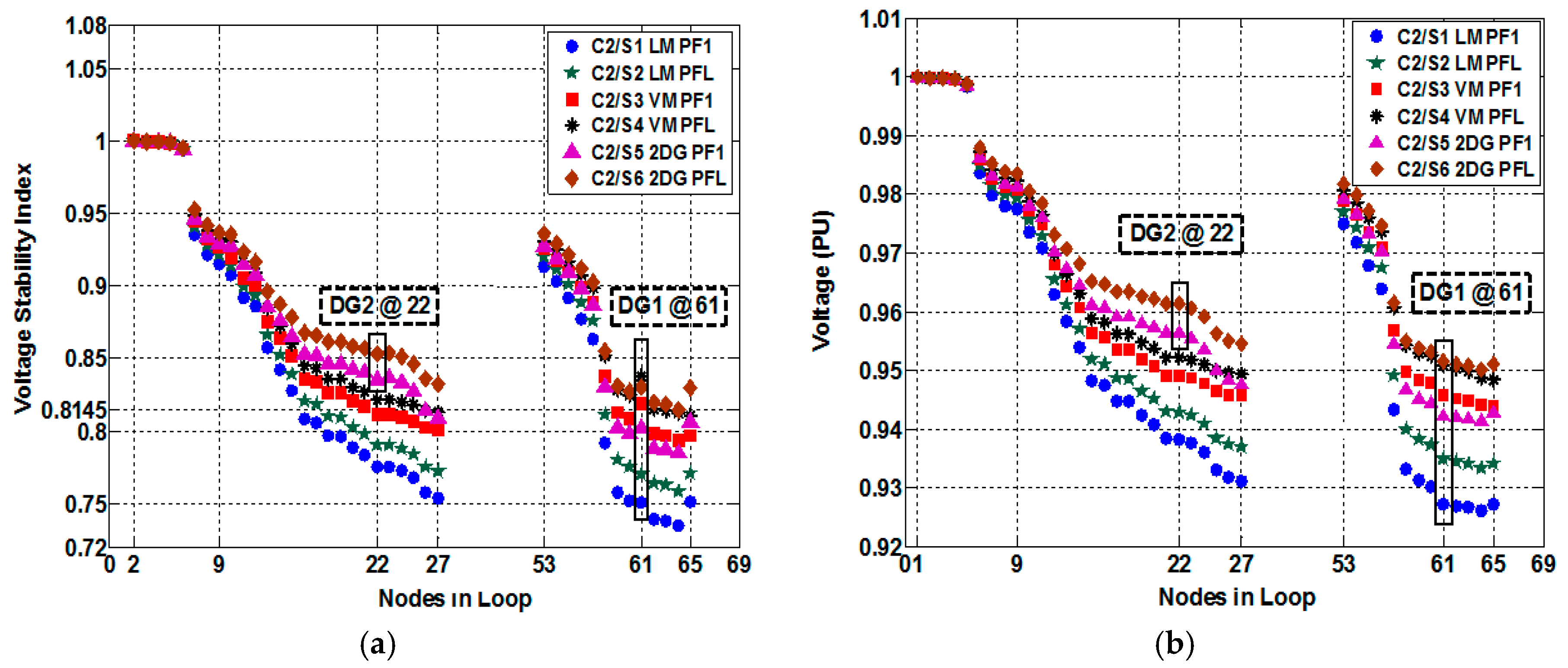
Run the power flow for test LDN at normal load, increase the capacity of DG (at PF1 or PFL = 0.82 ± 2%) in steps and calculate proposed VSI and V_R for real case at each node in loop according to Equations (1) and (2) i.e., resulting voltage at node with DG according to Equation (2) approaches close to 1.0 pu (nearly substation reference voltage); respectively. This step gives two scenarios for VM with single DG operating at PF1 and PFL (C1/S3 and C1/S4), respectively.

Step 3

Decrease the capacity of DG (at PF1 or PFL equal to 0.82 ± 2%) in steps and find out the LM according to Equations (9a) and (9b), respectively.

Step 4

When LMC with one DG has achieved according to Equations (9a) and (9b), i.e., the end-nodes across the TL (including TS) have the lowest difference of the numerical values VSI and V_R; according to Equations (1) and (2), respectively. The respective DG capacities and their operating power factors are the optimal choices. This step gives two scenarios (C1/S1 and C1/S2) for LM for single DG operating at PF1 and PFL, respectively.

Step 5

Repeat step 2 and place second DG in test LDN. Increase the capacity of DG at PF1 or PFL = 0.82 ± 2% in steps and calculate proposed VSI and V_R according to Equations (1) and (2), respectively.

Step 6

Decrease the capacity of DG1 and increase the capacity of DG2 in steps at PF1 or PFL equal to 0.82 ± 2%. Then find out the LM according to Equations (11a) and (11b), respectively.

Step 7

When LMC has achieved according to Equations (11a) and (11b), i.e., the end-nodes across the TL (including TS) have the lowest difference of the numerical values according to Equations (1) and (2), the condition has met the respective DG capacities and their power factors are the optimal choice. This step gives two scenarios (C1/S5 and C1/S6) for LM and VM with two DGs, each operating at PF1 and PFL, respectively.

3.2.2. Case 2: Impact of Same Distributed Generation Unit Capacity as Case 1 under Load Growth

Unlike case 1, case 2 has considered the impact of load growth (across 5 years) on aimed objectives, primarily VM and LM. The respective DG capacities from case 1 have retained constant and the load growth impact on VSI, system losses, and voltage profile have considered. The case 2 has further demonstrated with six scenarios and is discussed in the next section. The load growth is measured at a rate of 7.5% increase per year and planning period as 5 years, is also considered in [32]. The load model is same (CP-SLL) and modified load after load growth is 5459.124 KW and 3865.72 KVAR, respectively.

3.2.3. Case 3: Impact of Modified Distributed Generation Unit Capacity under Load Growth

The case 3 corresponds to optimal DG sizing at PF1 and PFL to eliminate load imbalance across feeders and I_TL in LDN under load growth scenarios. The aimed objectives include single and multiple DG placements under load growth for LM, VM and both, respectively. The considered conditions include modified load (CP-SLL with an allowable variation of ±2%) and modified DG capacity under load growth (5459.124 KW and 3865.72 KVAR), respectively.

The case 3 has further demonstrated in six scenarios and broadly discussed in next section. The impacts have shown as numerical values achieved in VSI, voltage profile, LM and various cost related performance indicators. The results have discussed and further compared with existing works available in the literature, in following sections. The computation procedure for case 3 is same as case 1, since, it offers the performance analysis of LDN with modified load after load growth and associated modified DG capacity to improve the system’s performance indicators, respectively.

4. Evaluation of Results and Discussion

In this section, evaluation of results aiming at the second variant of planning approach is further elaborated with three relevant cases and respective scenarios have discussed, respectively.

4.1. Evaluation of Results for Case 1

It has found that LDN without DG results in more losses than its radial counterpart. Besides the type, the suboptimal DG capacity can result in increased system losses in a DN. It has been observed that after looping without DG, the active losses in test LDN under normal load increases from 224.96 KW (in radial) to 260.736 KW, respectively. The reason includes high loop current flowing across the TL. The performance analysis of case 1 with six scenarios have illustrated in Figure 6a,b, where values of proposed VSI and voltage profile, after installing type-I and type-II DG at PF1 and PFL, have evaluated respectively.

In step 1, place first DG in LDN at node 61, on the basis of findings in variant 1 (case 0). According to step 2, the power flow of test LDN with one DG at respective power factor has run at normal load level. The DG capacity has increased in steps i.e., resulting VSI value according to Equation (1), corresponds to the voltage at the node with DG according to Equation (2), which must approaches close to 1.0 pu (nearly substation reference voltage); respectively.

Step 2 serves the performance analysis of two scenarios of VM in Figure 6a,b, with single DG placement in LDN at PF1 and PFL, designated in nomenclature as C1/S3 and C1/S4; respectively. The values of DGs have found to be 2309.250 KW at PF1 for C1/S3 and 2529.075 KVA at PFL with the numerical value of 0.82868 (PF) for C1/S4; respectively. The power flow from sub-station reduces to 1805.542 KW + j2769.6372 KVAR and 1793.524 KW + j1335.58445 KVAR for single DG operating at PF1 and PFL @ 0.82868, respectively. The active power losses reduce from 260.736 KW to 151.978 KW and 86.722 KW; and the loss reduction by percentage (P_LR%) corresponds to 41.712% and 66.74%; for C1/S3 and C1/S4, respectively. The respective DG penetration accounts for 60.73% for DG type-I in C1/S3 at PF1 and 54.28% for DG type-II at PFL in C1/S4, respectively.

The annual investment cost (AIC) of DGs, operating at various capacities (and PF) accounts for 0.6107 million USD per annum (one year) for DG type-I in C1/S3 at PF1 and 0.457 million USD per annum for DG type-II in C1/S4 at PFL (consult Table 1 for the simulation parameters values for AIC), respectively. In both VM scenarios, the voltage stability is high and from the viewpoint of VSI values and voltage profile. However, system losses reductions achieved in percentage are less from the perspective of other scenarios. The minimum VSI and voltage (PU) value in C1/S3 is 0.9224 and 0.9799 pu at node 22, respectively. Similarly, the minimum VSI and voltage (PU) value in C1/S4 is 0.9314 and 0.9822 pu at node 22, respectively.

The AIC of DG operating at various capacities (and PF) accounts for 0.45648 million USD per annum for DG type-I in C1/S1 at PF1 and 0.3650345 million USD per annum for DG type-II in C1/S2 at PFL, respectively. In both the scenarios (C1/S1 and C1/S2), the voltage stability is comparatively lower and from the viewpoint of VSI values and voltage profile, however loss minimizations achieved by percentage are greater from the perspective of other scenarios (C1/S3 and C1/S4). The minimum VSI and voltage (PU) value in C1/S1 is 0.8812 and 0.9687 pu at the end node 27, respectively. Similarly, the minimum VSI and voltage (PU) values in C1/S2 at end-node 27 across the TL are, 0.8971 and 0.9731; respectively.

According to Steps 5 and 6, repeat the step 2 and place the second DG (DG2) in test LDN. The capacity of DG2 needs to increase in steps at PF1 or PFL (equal to 0.82 ± 2%). The capacity of DG1 is required to simultaneously reducing in accordance with Equations (11a) and (11b), respectively.

On the basis of step 7, when the end-nodes across the TL (including TS) have the lowest difference of the numerical values according to Equations (1) and (2). At this stage, the LMC has achieved according to Equations (11a) and (11b). Also, the respective DG capacities and their associated power factors based on the scenarios are the optimal choices. The findings of Steps 5, 6 and 7 serve as the performance analysis of two scenarios for simultaneously achieving LM and VM with two DGs, each operating at PF1 and PFL, and shown in Figure 6a,b; respectively. The respective scenarios have designated in nomenclature as C1/S5 and C1/S6; respectively.

The DG capacities at PF1, from the perspective of scenario C1/S5, have found to be 1970.228 KW at node 61 for DG1 and 385.985 KW at node 22 for DG2; respectively. Likewise, DG capacities at PFL, in the context of scenario C1/S6, have found to be 2328 KVA at node 61 for DG1 and 400 KVA at the node 22 for DG2; respectively. The respective PFL for each DG (DG1 and DG2) in scenario C1/S6 have the numerical values of 0.8248 and 0.82426; respectively.

The power flow from sub-station reduces to 1527.389 KW + j2738.723 KVAR and 1578.284 KW + j1167.2987 KVAR for two DGs operating at PF1 and PFL @ 0.82, respectively. Hence, a considerable amount of capacity released from the substation has observed. The active power losses reduce from 260.736 KW to 80.998 KW and 25.367 KW; and the loss reduction by percentage corresponds to 68.935% and 90.27%; for C1/S5 and C1/S6, respectively. The respective DG penetration accounts for 61.96% for DG type-I in C1/S5 at PF1 and 58.55% for DG type-II at PFL in C1/S6, respectively.

The AIC of DG operating at various capacities (and PF) accounts for 0.62312 million USD per annum for DG type-I in C1/S5 at PF1 and 0.493 million USD per annum for DG type-II in C1/S6 at PFL, respectively. The minimum VSI and voltage (PU) value across TL in C1/S5 is, 0.9394 and 0.9839 pu at end node 65, respectively. Similarly, the minimum VSI value across TL in C1/S6 is 0.9620 and 0.9632 at the end-nodes 27 and 65, respectively. The minimum voltage values across TL in C1/S6 are 9903 pu each, at the end-nodes 27 and 65, respectively.

In the scenarios C1/S5 and C1/S6, voltage stability and system loss reductions are relatively better than previous scenarios. Also in comparison, scenario C1/S6 outperforms C1/S5 from the viewpoint of VSI values and voltage profile, LM, and AIC. However, C1/S5 offers higher DG penetration for type-II DG operating at PF1 in comparison with the C1/S6 scenario. It has been observed in Figure 6a that C1/S6 maintains stable VSI value with two DGs close to the ideal limit followed by C1/S5, C1/S3, and C1/S4, respectively. Furthermore, Figure 6b replicates in-terms of better voltage profile for the C1/S6 scenario. It has also found that LM with one DG (as in C1/S1 and C1/S2) can result in a reduction of the overall voltage profile. Hence, C1/S6 and C1/S5 performs better than other scenarios of case 1, among various performance indicators and represents a promising application for future LDN under smart grid paradigm.

4.2. Evaluation of Results for Case 2

It has been observed that under load growth across five years without DG, active losses increase from 224.96 KW to 506.5185 KW in radial; and 260.736 KW to 572.2015 KW in loop topology; respectively. The reason being high loop current flowing across the TL. The performance analysis of case 2 with six scenarios have illustrated in Figure 7a,b, where impacts of load growth at 7.5% [32] per year at same retained DG capacities as in case 1, have evaluated respectively. In order to keep discussion to the point, results with only fifth-year load profile have demonstrated in the analysis.

The values of DGs from case 1 have retained the same in case 2, i.e., 1726.102 KW at PF1 for C2/S1 and 2020.1833 KVA at PFL for C2/S2; respectively. The power flow from sub-station under load growth, increases to 4043.9579 KW + j4037.8648 KVAR, and 3915.746 KW + j2779.878 KVAR for single DG operating at PF1 and PFL; respectively. The active power losses in comparison with case-1, increases to 310.9359 KW and 113.208 KW; and the loss reduction by percentage corresponds to 45.66% and 80.21%; for C2/S1 and C2/S2, respectively. The respective DG penetration reduces to 31.62% for DG type-I in C2/S1 at PF1 and 30.20% for DG type-II at PFL in C2/S2, respectively.

The AIC of DG operating at various capacities have retained constant and accounts for the same as case 1. In both the scenarios (C2/S1 and C2/S2), the voltage stability is comparatively lower in terms of VSI values and voltage profile. Also, system losses increase in comparison with respective counterparts in case 1. The minimum VSI and voltage (PU) value in C2/S1 is 0.7349 and 0.9261 pu at node 64, respectively. Similarly, the minimum VSI and voltage values in C2/S2 accounts for 0.7581 and 0.9334 pu at the node 64, respectively. It has also observed that due to load growth, the LMC according to Equations (9) and (11) has relaxed. Reason being a reasonable amount of current flows through the TL and as a result, the end nodes (27 and 65) does not exhibit the lowest numerical values of VSI and V_R in accordance with Equations (1) and (2); respectively.

The performance analysis of two scenarios of VM is also presented in Figure 7a,b, with single DGP in LDN at PF1 and PFL, respectively. The VM scenarios designated in nomenclature as C2/S3 and C2/S4 at the same capacity as of case 1 (2309.250 KW at PF1 and 2529.075 KVA at PFL equal to 0.82 ± 2%) performs better under load growth than C2/S1 and C2/S2, respectively.

The power flow from sub-station reduces to 3350.0276 KW + j3969.307 KVAR and 3440.5956 KW + j2503.21 KVAR for single DG operating at PF1 and PFL, respectively. The active power losses reduce from 572.2015 KW to 200.38055 KW and 77.5186 KW; and the loss reduction by percentage corresponds to 64.98% and 86.45%; for C2/S3 and C2/S4, respectively. The respective DG penetration accounts for 42.30% for DG type-I in C2/S3 at PF1 and 37.81% for DG type-II at PFL in C2/S4, respectively.

The scenarios C2/S3 and C2/S4 in comparison with LM scenarios (C2/S1 and C2/S2), results in better the voltage stability from the viewpoint of VSI values and voltage profile. Furthermore, the LM achieved in percentage are more than C2/S1 and C2/S2 scenarios; respectively. The system losses vary as a function of DG penetration level in a U-shaped trajectory [32,34]. As the DG penetration increases, system losses reduce to a certain point and then it starts increasing. The high value of DG during normal loading for VM scenarios (C1/S3 and C1/S4) in case 1 has shifted towards close to loss minimization values (DGP versus LM in U-shaped trajectory) in case 2 during load growth, as shown in concerned scenarios C2/S3 and C2/S4, respectively. Hence, a trend for LM has observed in VM scenarios during load growth. The minimum VSI and voltage (PU) value in C2/S3 is 0.7936 at node 64 and 0.9439 pu at node 65, respectively. Similarly, the minimum VSI and voltage values in C2/S4 are 0.8111 and 0.94842 pu at node 65, respectively.

It has also been observed that during load growth, C2/S4 (VM scenario) corresponding to single DG operation at PFL seems to satisfy the LMC according to Equations (9a) and (9b), respectively. Also, the current flows through the TL reduces and end-node 65 (besides node 27) exhibits the lowest numerical values of VSI and V_R in accordance with Equations (1) and (2); respectively.

The performance analysis of two scenarios for LM and VM with two DGs in Figure 7a,b, under load growth (case 2), have designated in nomenclature as C2/S5 and C2/S6; respectively. The DG capacities at PF1 in C2/S5 have retained the same as in C1/S5.The reason is to study the load impact on load growth on system’s performance. The DG capacities in C2/S5 are 1970.228 KW at node 61 for DG1 and 385.985 KW @ node 22 for DG2; respectively. Likewise, DG capacities in C2/S6 are same as C1/S6 i.e., 2328 KVA at node 61 for DG1 and 400 KVA at node 22 for DG2; respectively.

The power flow from sub-station are, 3299.2665 KW + j3970.4695 KVAR and 3286.201 KW + j2372.9048 KVAR, for two DGs operating at PF1 and PFL, respectively. The active power losses reduce from 572.2015 KW to 196.08145 KW and 76.76 KW; and the loss reduction by percentage corresponds to 65.732% and 86.58%; for C2/S5 and C2/S6, respectively. The respective DG penetration accounts for 43.16% for DG type-I in C2/S5 at PF1 and 40.8% for DG type-II at PFL in C2/S6, respectively.

The AIC of DGs in case 2 has retained the same. Since DGs operate at the same capacity in case 2, similar to case 1 at the start of the planning period. The minimum VSI and voltage (PU) value in C2/S5 is 0.7851 and 0.94 pu at node 64, respectively. Similarly, the minimum VSI and voltage values in C2/S6 are 0.8143 at node 64 and 0.9502 pu at node 65, respectively. It has also observed that during load growth, C2/S6 corresponding to two DG operation at PFL seems close to the LMC according to Equations (11a) and (11b), respectively. However, still, the lowest numerical values of VSI and V_R in accordance with Equations (1) and (2); respectively have partially satisfied.

In the scenarios C2/S6, the voltage stability is comparatively better than all the previous scenarios in case 2. On the basis of overall comparison, scenario C2/S6 outperforms C2/S3, C2/S4, and C2/S5; from the viewpoint of VSI values and voltage profile, LM and AIC.

4.3. Evaluation of Results for Case 3

The performance analysis of case 3 has shown in Figure 8a,b, respectively. The two VM scenarios, designated in nomenclature as C3/S3 and C3/S4, aims at evaluation of LDN performance with single DG placement i.e., modified DGC (at PF1 and PFL) under load growth, respectively.

The values of DGs have found to be 3322.561 KW at PF1 for C3/S3 and 3645.5 KVA at PFL with the numerical value of 0.825 (PF) for C3/S4; respectively. The power flows from sub-station are 2350.8721 KW + j3971.26 KVAR and 2558.5169 KW + j1872.2372 KVAR for single DG operating at PF1 and PFL (0.825), respectively. The active power losses reduce from 572.2015 KW to 214.091 KW and 106.9169 KW; and the loss reduction by percentage (P_LR%) corresponds to 62.546% and 81.31%; for C3/S3 and C3/S4, respectively. The respective DG penetration (DG%) accounts for 60.8625% for DG type-I in C3/S3 at PF1 and 54.5% for DG type-II at PFL in C3/S4, respectively.

The AIC associated with DGs operating at various capacities accounts for 0.87868 million USD per annum for DG type-I in C3/S3 at PF1 and 0.65872 million USD per annum for DG type-II in C3/S4 at PFL, respectively. The minimum VSI and voltage value in C3/S3 is 0.8735 and 0.9666 pu at node 22, respectively. Similarly, the minimum VSI and voltage values in C3/S4 are 0.888 and 0.9706 pu at node 22, respectively.

The performance analysis of two LM scenarios are shown in Figure 8a,b, with single DG placement in LDN at PF1 and PFL, and designated in nomenclature as C3/S1 and C3/S2; respectively. The capacities of single DG (in C3/S1 and C3/S2) have decreased to meet the LMC according to Equations (9a) and (9b), and end-nodes across the TL (including TS) have the lowest numerical values of VSI and V_R; according to Equations (1) and (2); respectively.

The values of DG capacity has found to be 2498.05 KW at PF1 for C3/S1 and 2772.657 KVA at PFL with the numerical value of 0.8232 for C3/S2; respectively. The power flows from sub-station in C3/S1 and C3/S2, reduces to 3137.9363 KW + j3967.85 KVAR and 3227.4756 KW + j2350.6107 KVAR for single DG operating at PF1 and PFL at 0.8232, respectively. The active power losses reduce from 572.2015 KW to 176.8623 KW and 50.8846 KW; and the P_LR% corresponds to 69.1% and 91.10%; for C3/S1 and C3/S2, respectively. The respective DG penetration accounts for 45.76% for DG type-I in C3/S1 at PF1 and 41.45% for DG type-II at PFL in C3/S2, respectively.

The AIC of DG units operating at respective capacities accounts for 0.66063 million USD per annum for DG type-I in C3/S1 at PF1 and 0.501 million USD per annum for DG type-II in C3/S2 at PFL; respectively. In both the C3/S1 and C3/S2 scenarios, voltage stability is comparatively lower from the viewpoint of VSI values and voltage profile. However, losses reduction achieved in percentage are greater from the perspective of other (C3/S3 and C3/S4) scenarios. The minimum VSI and voltage (PU) value in C3/S1 is 0.8138 and 0.9491 pu at the end node 65, respectively. Similarly, the minimum VSI values and voltage values in C3/S2 are 0.8311 at end-node 27 and 0.9547(PU) at end-node 65 across the TL (including TS) in LDN, respectively.

The performance analysis of two scenarios for LM and VM with two DGs, designated in nomenclature as C3/S5 and C3/S6, each set operating at PF1 and PFL; is shown in Figure 8a,b; respectively. The DG capacities at PF1, from the perspective of scenario C3/S5, have found to be 2881.596 KW at node 61 for DG1 and 526.027 KW at node 22 for DG2; respectively. Likewise, DG capacities at PFL, in the context of scenario C3/S6, have found out to be 3347.56 KVA at node 61 for DG1 and 497.06 KVA at node 22 for DG2; respectively. The respective PFL for each DGs at node 61 and 22, in scenario C3/S6, have the numerical values of 0.8292 and 0.8251; respectively.

The power flows from sub-station in C3/S5 and C3/S6, reduces to 2222.4844 KW + j3962 KVAR and 2320.8792 KW + j1743.2942 KVAR for two DGs operating at PF1 and PFL, respectively. The active power losses reduce from 572.2015 KW to 170.9834 KW and 47.85925 KW; and P_LR% corresponds to 70.12% and 91.64%; for C3/S5 and C3/S6, respectively. The DG penetration accounts for 62.42% for DG type-I in C3/S5 at PF1 and 57.475% for DG type-II at PFL in C3/S6, respectively.

The AIC of DG operating at various capacities and power factors accounts for 0.901172 million USD per annum for DG type-I in C3/S5 at PF1 and 0.6947 million USD per annum for DG type-II in C3/S6 at PFL, respectively. The minimum VSI and voltage (PU) value across TL in C3/S5 is 0.9003 and 0.9732 pu at the end node 65, respectively. Similarly, the minimum VSI and voltage values across TL in C3/S6 are 0.9212 at the end-nodes 27 and 0.9794 at the end-nodes 65, respectively.

5. Performance Analysis and Comparison of Results

5.1. Performance Analysis of the Proposed Planning Approach

The results of the proposed approach (variant 2) have arranged in a complete package in terms of performance indicators, as shown in

Table 2. Overall complete overview of performance analysis.

Case (No.)/Scenario (No.)	DG Size (KW/KVA)	Loc./PF. (Node/PF Value)	LM (KW + jKVAR)	DG% Penetration	Capacity Release (SS) (KW + jKVAR)	AIC (Million USD$)	P_LR (%)	CPL in (Million USD$)	Minimum VSI (Node)	Min. Voltage (Node)	No. of Application
C1/S1	1726.102 KW	61/PF1	83.275 + j41.27	45.39%	2159.773 + j2733.875	0.45648	68.06%	0.04377	0.8812/@27	0.9687/@65	1 LM
C1/S2	2020.2 KVA	61/0.82L	25.686 + j15.9	43.36%	2170.523 + j1552.488	0.3650345	90.15%	0.0135	0.8971/@27	0.9731/@27	1 LM
C1/S3	2309.25 KW	61/PF1	151.98 + j76.94	60.73%	1805.542 + j2769.637	0.6107	41.712%	0.07988	0.9224/@22	0.9799/@22	1 VM
C1/S4	2529.1 KVA	61/0.828L	86.722 + j58.46	54.28%	1793.524 + j1335.584	0.457	66.74%	0.0456	0.9314/@22	0.9822/@22	1 VM
C1/S5	1970.228 KW 385.985 KW	61/PF1 22/PF1	80.998 + j46.05	61.96%	1527.389 + j2738.723	0.62312	68.935%	0.0426	0.9394/@65	0.9839/@65	2 VM & LM
C1/S6	2328 KVA 400 KVA	61/0.825L 22/0.824L	25.367 + j17.26	58.55%	4043.9579 + j4037.864	0.493	90.27%	0.013333	0.9620/@27 0.9632/@65	0.9903/@27 0.9903/@65	2 VM & LM
C2/S1	1726.102 KW	61/PF1	310.94 + j172.1	31.62%	3915.746 + j2779.878	0.45648	45.66%	0.163428	0.7349/@64	0.9261/@64	-
C2/S2	2020.2 KVA	61/0.82L	113.21 + j70.6	30.20%	3350.0276 + j3969.307	0.3650345	80.21%	0.05950	0.7581/@64	0.9334/@64	-
C2/S3	2309.25 KW	61/PF1	200.38 + j103.5	42.30%	3440.5956 + j2503.21	0.6107	64.98%	0.10532	0.7936/@64	0.9439/@64	-
C2/S4	2529.1 KVA	61/0.828L	77.5186 + j53.7	37.81%	3299.2665 + j3970.469	0.457	86.4526%	0.040744	0.8111/@65	0.9484/@65	1 LM
C2/S5	1970.228 KW 385.985 KW	61/PF1 22/PF1	196.08 + j103.9	43.16%	3286.201 + j2372.905	0.62312	65.732%	0.10306	0.7851/@64	0.9414/@64	-
C2/S6	2328 KVA 400 KVA	61/0.825L 22/0.824L	76.76 + j49.846	40.80%	4043.9579 + j4037.865	0.493	86.58%	0.040345	0.8143/@64	0.9502/@65	2 VM & LM
C3/S1	2498.05 KW	61/PF1	176.86 + j102.1	45.76%	3137.9363 + j3967.85	0.66063	69.1%	0.09296	0.8138/@65	0.9491/@65	1 LM
C3/S2	2772.66 KVA	61/0.823L	50.88 + j31.952	41.45%	3227.4756 + j2350.61	0.501	91.1%	0.026745	0.8311/@27	0.9547/@65	1 LM
C3/S3	3322.561 KW	61/PF1	214.31 + j105.5	60.8625%	2350.8721 + j3971.26	0.87868	62.546%	0.11264	0.8735/@22	0.9666/@22	1 VM
C3/S4	3645.5 KVA	61/0.825L	106.92 + j66.73	54.50%	2558.5169 + j1872.237	0.65872	81.31%	0.0592	0.8880/@22	0.9706/@22	1 VM
C3/S5	2881.596 KW 526.027 KW	61/PF1 22/PF1	170.98 + j96.2	62.42%	2222.4844 + j3962	0.901172	70.12%	0.08987	0.9003/@65	0.9732/@65	2 VM & LM
C3/S6	3347.56 KVA 497.06 KVA	61/0.829L 22/0.825L	47.86 + j29.252	57.475%	2320.8792 + j1743.294	0.6947	91.64%	0.025155	0.9212/@27 0.9216/@65	0.9794/@65 0.9796/@27	2 VM & LM

. The main purpose of the summary is to provide quick information regarding findings of the proposed technique and discuss important features, respectively. The performance analysis considers the following evaluation indicators as follows.

• DG capacities (DGC) in each case: The DG capacities, numbers, locations, operating power factors, and applications; utilized in the performance analysis of all cases (1–3) and their relevant scenarios (1–6); have summarized in Table 2.
• Active and reactive loss minimizations: It has found that scenario 6 in all cases (1–3) outperforms their relative counterparts from the perspective of LM. It is worth-mentioning that single DG for LM follows Equation (9). Whereas, two DGs for LM, requires to obey Equation (11).
• DG Penetration (DG%) in loop distribution network: It has been observed that scenario 5 in all cases (1–3) outperforms their relative counterparts from the perspective of DG penetration, in particular, type-I DG operating at PF1 and represents the application of renewable energy generation (REG) such as photovoltaic power based DG [34].
• Capacity Release from sub-station in loop distribution network: It has been observed that scenario 6 in all cases (1–3) outperforms their relative counterparts from the perspective of capacity release in distribution network due to the reduction of power flows from the substation with two DGs at optimal location and size, respectively.
• Annual investment cost (AIC) of distributed generation units: The annual investment cost (AIC) for DGs operating at respective PF (by type) in each case is shown in million USD ($). It has found that scenario 2 perform better among the two scenarios for LM with single DG. Similarly, scenario 4 in all cases performs better among the two scenarios for VM with single DG. However, high AIC values for scenario 6 in comparison with other scenarios seems justified due to the application of simultaneous VM and LM, with two DGs placed at the optimal location and relative capacity, respectively.
• Active power loss reduction by percentage (P_LR): It has been observed that scenario 6 in all cases (1–3) outperforms their relative counterparts from the perspective of active power loss reduction in LDN by percentage. The reason is a reduction of power flows from the substation and active and reactive powers are fed directly to the loads with two DGs at the optimal location, size, and PFL; respectively.
• The cost of Active Power losses (CPL): The cost of active power losses (CPL) have presented in million USD ($), with DG operating at relevant PFs in each case, respectively. It has been observed that scenario 6 in all cases (1–3) outperforms their relative counterparts from the perspective of CPL aiming at the application of LM, with two DGs in LDN.
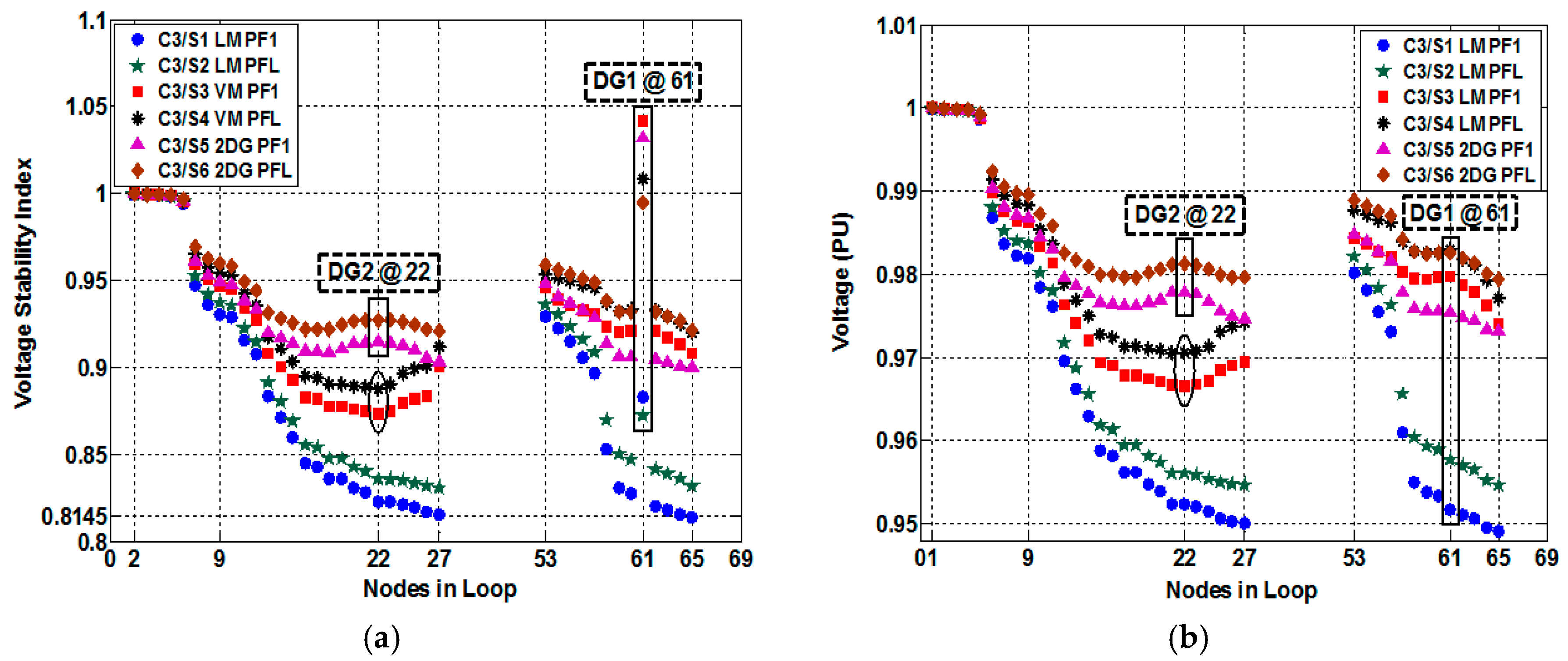
• Analysis of VSI values and Voltage Profile: It has been observed that during normal loading scenarios in case 1 and load growth scenarios in case 3; scenario 6 outperforms the other respective scenarios from the perspective of better VSI values and voltage profile. Thus, satisfying both the LMC (Equations (11a) and (11b)) and VM conditions (Equations (1) and (2)), as aforementioned in the variant 2 of proposed planning approach (Section 4), respectively.

However, it has been observed during load growth that only C2/S4 satisfies the LM conditions rather than VM as in previous C1/S4 scenario, respectively. The reason is a variation of system losses as a function of DG penetration (DG%) level follows a U-shaped trajectory. As DG% increases, loss minimizes to a certain point and then it starts increasing. The high value of DG during normal loading scenario of C1/S4 for VM cases has shifted towards close to LM values in C2/S4 during load growth, respectively. It has been observed that only C2/S4 scenario among other scenarios of case 2 satisfies the minimum numerical values of VSI and voltage according to Equations (1) and (2). Also, the LMC in C2/S4 is considered feasible with one DG is in accordance with Equations (9a) and (9b) and partially feasible in C2/S6 with Equations (11a) and (11b), respectively.

5.2. Comparison of the Results

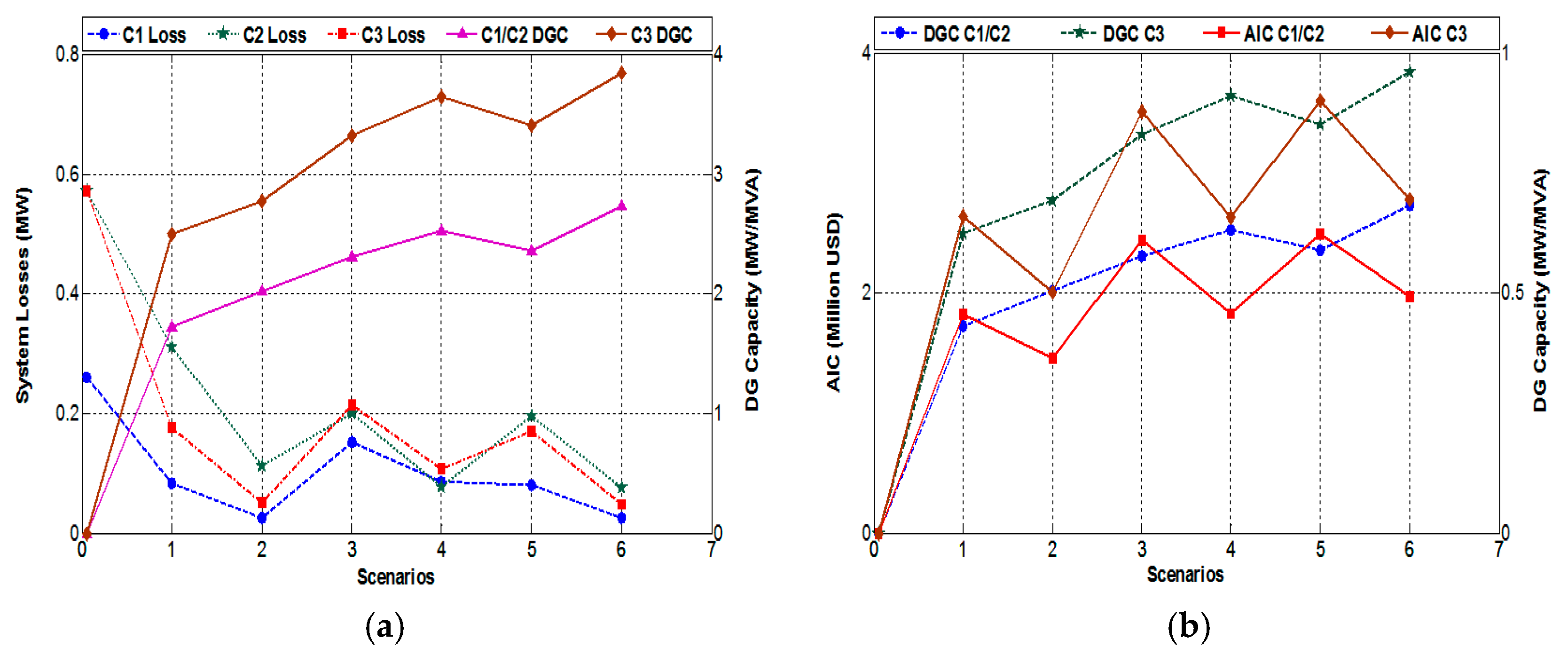
5.2.1. Active (System) Losses Reduction vs. Distributed Generation Capacity

In this sub-section, a concluding comparison of system (active) losses minimization versus DG capacities (DGC) for each case and respective scenarios are demonstrated in Figure 9a as a comprehensive analysis. It has been observed that scenario C1/S6 in case 1, during normal loading capacity, results in better performance from the viewpoint of system loss (designated as C1 Loss) to DG capacity (designated as C1 DGC). Since VM and LM are two conflicting objectives in various aspects. Hence, the maximum difference among the two performance indicators visually shows the best solution among available options. The greater distance among C1 Loss and C1 DGC has found at scenario C1/S6 and thus it is the best solution during normal loading (case 1).

Similarly, in case 2, both scenarios C2/S4 and C2/S6 both perform well from the viewpoint of LM. However, C2/S4 shows more promising results from the perspective of LM in accordance with Equations (9a) and (9b). Moreover, it results in minimum VSI and voltage values for nodes across the TL in accordance with Equations (1) and (2); respectively. In simple words, it is observed in case 2 that scenario C2/S4 during load growth, results in better performance from viewpoint of LM, i.e., it deflects more close to the downside of (DGC vs. LM based U-shaped) curve. The loss and DG capacity in case 2 have designated as C2 Loss and C2 DGC (same as C1 DGC), respectively.

Finally, it has been observed in case 3 that scenario C3/S6 during modified loading capacity under load growth, results in better performance from the viewpoint of system loss (designated as C3 Loss) to DG capacity (designated as C3 DGC). The greater distance among C3 Loss and C3 DGC has found at scenario C3/S6. Thus, the best solution during modified load during load growth is C3/S6 that replicates the same as C1/S6 does during normal loading case 1, respectively. Likewise, it has been observed in Figure 9a that C1/S5 and C3/S5 scenarios with type-I DGs result in higher LM at comparatively high capacities, in comparison with their respective counterparts (PF1), respectively.

5.2.2. Annual Investment Cost (AIC) vs. Distributed Generation Capacity (DGC)

Another concluding comparison of overall AIC versus DG capacities (DGC) for each case and respective scenarios is demonstrated in Figure 9b as a comprehensive analysis. Since cost is an important factor in planning during load growth. Hence, it is important to observe the economic viability and feasibility of available solution in the context of cost analysis. It has been observed that for each respective scenario, the AIC versus DGC follows a zigzag sort of path. The DGC for each case (1–3) have designated with DGC C1, DGC 2 and DGC 3; respectively. Similarly, AIC for each case (1–3) has designated with AIC C1, AIC C2, and AIC C3; respectively. Also, as indicated in Table 2, it has found that scenario 2 perform better among the two scenarios for LM at the comparatively lower numerical value of AIC with single DG. The scenario 6 in both cases 1 and 3, justifies comparatively high AIC versus higher DGC, by outperforming other scenarios for the perspective of VM and LM (with two DGs), respectively.

5.2.3. Comparison of the Results with the Existing Research Works

The validation of proposed VSI–LMC based approach is carried out by comparing the achieved results with other VSI and sensitivity based approaches, as shown in

Table 3. Comparisons of results with other techniques under normal load at PF1.

Performance Indicators	[29]	[23]	[32]	C1/S1	C1/S5
DG Location	61	61	61	61	61, 22
DG Size (KW)	1863.1	1832.45	1870	1726.102	1970.228, 385.985
DG quantity	1	1	1	1	2
P-loss (KW)	83.142	83.195	83.13942	83.275	80.998
Q-loss (KVAR)	40.512	40.58	40.50	41.268	46.051
V-Min (bus)	0.968@26	0.968@26	0.968@26	0.9687@65	0.9839@65
VSI-Min (bus)	0.86555@57	0.8642@57	0.86585@57	0.8812@27	0.9394@65
CEL ($)	43700	43727	43698.1	43769.34	42572.55
CEL savings ($)	74491	74464	74493	74469.64	75634.89
DG capacity (MW)	1863.1	1832.45	1870	1726.102	2356.213
DG Penetration (%)	49	48.19	49.18	45.39	61.96

, i.e., RDN based VSI in [32], power stability index (PSI) [29] and novel power loss sensitivity (NPLS) [23] based methods. The compared methods were initially proposed for RDNs and have compared with LDN from the perspective of voltage stability, LM, DG penetration, DG quantity and respective savings; give a broad insight of the analysis, respectively.

It has found that single DG placement in the LDN for the application of LM in scenario C1/S1 results in active loss reduction in close agreement with other techniques at comparatively less capacity. Also, the voltage profile and VSI values are better than the compared techniques. Although the cost of energy losses (CEL) are high in LDN, however, it can be considered at the cost of reliability from the viewpoint of serving consumer with stable voltage and reliable alternative. The LDN in C1/S5 scenario outperforms the respective techniques from the viewpoint of more active LM, less CEL, comparatively high savings, better voltage and VSI value, more capacity release and above all higher DG penetration at PF1 (indicating promising placement of photovoltaic based renewable DG) from the prospect of future smart distribution network under smart grid paradigm.

The proposed approach under normal load has been compared with VSI and genetic algorithm (GA) based intelligent methods, considering DG operating at various PFs and has shown in

Table 4. Comparisons with related techniques under normal load at various power factors (PF).

Indicators	[32] PF1	[34] PF1	[34] PFL	C1/S5 PF1	C1/S6 PFL
DG Location	61	61, 22	61, 22	61, 22	61, 22
DG Size (KW/KVA)	1870	1757; 491	2147; 590	1970.23; 386	2328; 400
DG quantity	1	2	2	2	2
P-loss (KW)	83.13942	99.9	23.4	80.998	25.367
Q-loss (KVAR)	40.50	-	-	46.051	17.2607
V-Min (bus)	0.968@26	-	-	0.9839@65	0.9903@65
VSI-Min (bus)	0.866@57	-	-	0.9394@65	0.9620@27
CEL ($)	43,698.1	52,507.44	12,299.04	42,572.55	13,332.9
CEL savings ($)	74,493	65,700	105,908.4	75,634.89	104,874.55
Loss Reduction (%)	63.03	61.70	91.03	68.935	90.27
AIC (Million USD)	0.4945	0.5946	0.4945	0.62312	0.493
DG capacity (MW)	1870	2248	2737	2356.213	2728
DG Penetration (%)	49.18	59.12	58.74	61.96	58.55

; respectively. The results of proposed approach have found in agreement with especially DG locations, DG penetration, AIC, LM and percentage loss reductions; in LDN from planning perspective as in [34], respectively. The scenario C1/S5 indicates that more active LM has obtained with proposed method, considering two DGs operating at PF1, as compared to work in [34]. The results of scenario C1/S6, considering two DGs operating at PFL, represent better evaluation than C1/S5 from the perspective of aforementioned performance indicators. However, a minor variation in DG capacity has observed with the proposed work, from the viewpoint of compared work in literature. On the basis of results obtained from proposed approach and other compared works, considering DGs (operating at PF1 and PFL), different DG locations and sizes can be achieved, as advocated in [23], respectively. Moreover, different methods result in various values of LM and voltage profile, respectively. Hence, the results obtained (cases 1–3 and respective six scenarios each) and presented here are specific to the proposed approach (variant 2). Note, the scale values of losses in [34] have considered, from the viewpoint for balanced 3-phase to 1-phase analogy, respectively. Besides, on the basis of genre, VSI-LMC based approach out performs their traditional counterparts from the viewpoint of achieving more objectives with multiple DG placement in LDN, respectively.

Table 5. Comparisons of results with other techniques under normal load at PFL.

Indicators	[32]	C1/S2	C1/S4	C1/S6
DG Location	61	61	61	61, 22
DG Size (KW)	2240	2020.2	2529.075	2328, 400
DG quantity	1	1	1	2
P-loss (KW)	23.124	25.686	86.722	25.367
Q-loss (KVAR)	14.363	15.8985	58.4595	17.2607
V-Min (bus)	0.954425@26	0.9731@27	0.9822@22	0.9903@65
VSI-Min (bus)	0.8083@57	0.8971@65	0.9314@22	0.9620@27
CEL ($)	12,154	13,500.56	45,581.1	13,332.9
CEL savings ($)	106,053.5	10,4706.9	72,626.4	104,874.55
DG capacity (MW)	2240	2020.2	2529.075	2728
DG Penetration (%)	48.07	43.36	54.28	58.55

indicates the results of the proposed approach, considering single and two DGs operating at PFL, and relative comparison from the perspective of various performance indicators, respectively. The scenario C1/S6 outperforms all PFL related DG scenarios and related work, in terms of achieving a high number of objectives in comparison. Likewise, the impact of load growth has been demonstrated in

Table 6. Comparisons of results with other techniques under load growth (5 years) at PF1.

Indicators	[32] 5 Year	C3/S1 5 Year	C3/S3 5 Year	C3/S5 5 Year
DG Location	61	61	61	61, 22
DG Size (KW)	2720	2498.05	3322.561	2881.6, 526.03
DG quantity	1	1	1	2
P-loss (KW)	175.1943	176.8623	214.3091	170.9834
Q-loss (KVAR)	85.12873	102.1297	105.5353	96.2307
V-Min (bus)	0.954425@26	0.9491@65	0.9666@22	0.9732@65
VSI-Min (bus)	0.8083@57	0.8138@65	0.8735@22	0.9003@65
CEL ($)	92,082.12	92,958.82	112,640.863	89,868.875
CEL savings ($)	173,830	173,267.36	153,585.26	176,357.25
DG capacity (MW)	2720	2498.05	3322.561	3407.623
DG Penetration (%)	49.84	45.76	60.86	62.42

and

Table 7. Comparisons of results with other techniques under load growth (5 years) at PFL.

Indicators	[32] 5 Year PFL	C3/S2 5 Year	C3/S4 5 Year	C3/S6 5 Year
DG Location	61	61	61	61, 22
DG Size (KW)	3230	2772.657	3645.50	3347.56; 497.1
DG quantity	1	1	1	2
P-loss (KW)	48.45194	50.8846	106.9169	47.85925
Q-loss (KVAR)	29.92891	31.9527	66.7342	29.2522
V-Min (bus)	0.960506@26	0.9547@65	0.9706@22	0.9794@65
VSI-Min (bus)	0.85093@26	0.8311@27	0.888@22	0.9212@27
CEL ($)	25,466.34	26,745	56,195.52	25,154.82
CEL savings ($)	240,441.27	239,481.2	210,030.6	241,071.3
DG capacity (MW)	3230	2772.657	3645.50	3844.62
DG Penetration (%)	48.29	41.45	54.50	57.48

. The obtained results for case 3 and scenarios 1, 3 and 5 have compared with [32]; considering DGs operating at PF1, and tabulated in Table 6. The C3/S5 seems to outperform among the relevant scenarios. Similarly, results in case 3 for scenarios 2, 4 and 6 have compared [32]; considering DG operating at PFL, and tabulated in Table 7, respectively. The C3/S6 has observed to outperform among the relevant scenarios and compared method, from the perspective of demonstrated performance indicators. On the basis of obtained and compared results for test DN (at PFL and PF1), it has been observed that locations of DG are the same. However, DG unit capacities vary. Hence, different LM, VM, and associated objective values have obtained.

The proposed planning method has been compared with available works in literature and the results obtained have been found to be in close agreement. Simulation results verify the validity of the proposed approach. In addition, numerical results show that LDN has shown more resilience and robustness than its RDN, both in terms of performance analysis and planning under the impact of load growth (across 5 years), respectively. It has been observed that two DG placement in LDN has resulted in high DG penetration, VM, LM, and associated objectives, in comparison with RDN. It has also found that two DGs with respective scenarios (C1/S5–S6, C3/S5–S6) in LDN can be utilized for; voltage control (regulation) in coordination with substation having on-load-tap-changers (OLTP) and facilitates more DG penetration, which is an important anticipated feature of SDN. Hence, loop system can be safely considered as a potential candidate for smart distribution network under SG paradigm on the basis of better performance than its radial counterpart. Moreover, it can provide a trade-off option among radial and mesh structure of distribution network, due to reliability and fault traceability, respectively. In future, LDN based planning problem will be extended to MDN, microgrid and interconnected MV-LV distribution system planning. Furthermore, the application of the proposed planning approach will also be addressed from the perspective of various voltage dependent characteristics of loads by type and multi-criteria (objective) based optimization in SG environment.

6. Conclusions

The planning tools proposed for RDN might not remain applicable to LDN. Hence on the basis of limitations, a new VSI and LMC based planning approach have proposed. The aim of VSI-LMC planning approach is to, access evaluation of LDN under various performance indicators; and supported with respective mathematical proofs. Initially, VSI relationship for equivalent LDN model has employed to find out potential locations for DG placement in LDN. Later, loss minimization formulations have been derived on the basis of an equivalent electrical model of LDN, for single and two DGs operating at various power factors, respectively. The assessment of LMC with single and two DGs under unity that have lagging power factors have also presented. The proposed planning approach is presented with two variants. In the first variant, also indicated as case 0, the optimal DG unit location and relevant capacities have found in a simplistic manner. The results indicate that LDN supports more DG penetration with two DGs placed at optimal capacities such that the current flowing through the tie-line is ideally close to zero. Also, the DG units operating at lagging power factor (or type-II DG) close to the lagging power factor of test distribution network result in better voltage stability and improved system loss minimizations than their counterparts operating at unity power factor. The reason being that the reactive power support provided by type-II DG has a positive impact on voltage stability and loss minimization since a considerable portion of reactive power by DGs has fed to loads rather than substation. Later, the second variant of planning approach is presented with three cases, each with six planning scenarios. Case 1 offers impact of DGs on test distribution network under normal load scenario. In case 2, the DG capacities in case 1 have kept constant and the impact of load growth (5 years) has studied across various performance indicators. In case 3, the modified DG capacities on the basis of planning approach, which is required to accommodate the load growth impact, have presented. The evaluation of the second variant of proposed planning approach offers a profound analysis of planning under various scenarios and the results indicate the favorable suitability of LDN for future application. The performance analysis of variant 2 has been conducted across prominent evaluation parameters found in literature, such as achieved DG capacities, active/reactive loss minimizations, DG penetration level, capacity release from the substation, annual investment cost, active power loss reduction achieved, cost of losses, values of VSI and voltage profile, with the proposed approach, respectively. Furthermore, a detailed result evaluation of variant 2 with single and two DG placement under various performance indicators have illustrated as a comprehensive analysis. The simulation results obtained have compared and found in close agreement with exited works available in literature and thus validates the proposed approach. Besides, LDN outperforms RDN from the perspective of aforementioned performance indicators. Since the limitations found in the TG have expected to be met with state-of-the-art technologies of the SG. Hence, the planning approach demonstrates the suitability of LDN (in terms of load growth) for future SDN-based applications under SG paradigm.

References

1. Rodriguez, A.A.; Ault, G.; Galloway, S. Multi-Objective planning of distributed energy resources: A review of the state-of-the-art. Renew. Sustain. Energy Rev. 2010, 14, 1353–1366. [Google Scholar] [CrossRef]
2. Fang, X.; Misra, S.; Xue, G.; Yang, D. Smart grid—The new and improved power grid: A survey. IEEE Commun. Surv. Tutor. 2012, 14, 944–980. [Google Scholar] [CrossRef]
3. Kalambe, S.; Agnihotri, G. Loss minimization techniques used in distribution network: Bibliographic survey. Renew. Sustain. Energy Rev. 2014, 29, 184–200. [Google Scholar] [CrossRef]
4. Sayed, M.A.; Takeshita, T. Line Loss Minimization in Isolated Substations and Multiple Loop Distribution Systems Using the UPFC 2014. IEEE Trans. Power Electron. 2014, 29, 5813–5822. [Google Scholar] [CrossRef]
5. Kim, J.C.; Cho, S.M.; Shin, H.S. Advanced Power Distribution System Configuration for Smart Grids. IEEE Trans. Smart Grid 2013, 4, 353–358. [Google Scholar] [CrossRef]
6. Kazmi, S.A.A.; Shahzad, M.K.; Khan, A.Z.; Shin, D.R. Smart Distribution Networks: A Review of Modern Distribution Concepts from Planning Perspectives. Energies 2017, 10, 501. [Google Scholar] [CrossRef]
7. Keane, A.; Ochoa, L.F.; Borges, C.L.T.; Ault, G.W.; Alarcon-Rodriguez, A.D.; Currie, R.; Pilo, F.; Dent, C.; Harrison, G.P. State-of-the-art techniques and challenges ahead for distributed generation planning and optimization. IEEE Trans. Power Syst. 2013, 28, 1493–1502. [Google Scholar] [CrossRef]
8. Georgilakis, P.S.; Hatziargyriou, N.D. A review of Power distribution planning in the modern power systems era: Models, methods, and future research. Electr. Power Syst. Res. 2015, 121, 89–100. [Google Scholar] [CrossRef]
9. Evangelopoulos, V.A. Optimal operation of smart distribution networks: A review of models, methods, and future research. Electr. Power Syst. Res. 2016, 140, 95–106. [Google Scholar] [CrossRef]
10. Ju, Y.; Wu, W.; Zhang, B.; Sun, H. Loop-analysis-based continuation power flow algorithm for distribution networks. IET Gener. Transm. Distrib. 2014, 8, 1284–1292. [Google Scholar] [CrossRef]
11. Sultanaa, U.; Khairuddin, A.B.; Aman, M.M.; Mokhtara, A.S.; Zareen, N. A review of optimum DG placement based on minimization of power losses and voltage stability enhancement of distribution system. Renew. Sustain. Energy Rev. 2016, 63, 363–378. [Google Scholar] [CrossRef]
12. Mehmood, K.K.; Khan, S.U.; Lee, S.J.; Haider, Z.M.; Rafique, M.K.; Kim, C.H. Optimal sizing and allocation of battery energy storage systems with wind and solar power DGs in a distribution network for voltage regulation considering the lifespan of batteries. IET Renew. Power Gener. 2017. [Google Scholar] [CrossRef]
13. Georgilakis, P.S.; Hatziargyriou, N.D. Optimal Distributed Generation Placement in Power Distribution Networks: Models, Methods, and Future Research. IEEE Trans. Power Syst. 2013, 28, 3420–3428. [Google Scholar] [CrossRef]
14. Jordehi, A.R. Allocation of distributed generation units in electric power systems: A review. Renew. Sustain. Energy Rev. 2015, 56, 893–905. [Google Scholar] [CrossRef]
15. Prakash, P.; Khatod, D.K. Optimal sizing and sitting techniques for distributed generation in distribution systems: A review. Renew. Sustain. Energy Rev. 2016, 57, 111–130. [Google Scholar] [CrossRef]
16. Sedghi, M.; Ahmadian, A.; Golkar, M.A. Assessment of optimization algorithms capability in distribution network planning: Review, comparison and modification techniques. Renew. Sustain. Energy Rev. 2016, 66, 415–434. [Google Scholar] [CrossRef]
17. Kazmi, S.A.A.; Shahzad, M.K.; Shin, D.R. Multi-Objective Planning Techniques in Distribution Networks: A composite Review. Energies 2017, 10, 208. [Google Scholar] [CrossRef]
18. Modarresi, J.; Gholipour, E.; Khodabakhshain, A. A comprehensive review of the voltage stability indices. Renew. Sustain. Energy Rev. 2016, 63, 1–12. [Google Scholar] [CrossRef]
19. Ettehadi, M.; Ghasemi, H.; Vaez-Zadeh, S. Voltage stability-based DG placement in distribution networks. IEEE Trans. Power Deliv. 2013, 28, 171–178. [Google Scholar] [CrossRef]
20. Quezada, V.M.; Abbad, J.R.; Roman, T.G.S. Assessment of energy distribution losses for increasing penetration of distributed generation. IEEE Trans. Power Syst. 2006, 21, 533–540. [Google Scholar]
21. Hung, D.Q.; Mithulananthan, N.; Bansal, R.C. Analytical strategies for renewable distributed generation integration considering energy loss minimization. Appl. Energy 2013, 105, 75–85. [Google Scholar] [CrossRef]
22. Hung, D.Q.; Mithulananthan, N. Loss reduction and loadability enhancement with DG: A dual-index analytical approach. Appl. Energy 2014, 115, 233–241. [Google Scholar] [CrossRef]
23. Murthy, V.V.S.N.; Ashwani, K. Comparison of optimal DG allocation methods in radial distribution systems based on sensitivity approaches. Electr. Power Energy Syst. 2013, 53, 450–467. [Google Scholar] [CrossRef]
24. Murthy, V.V.S.N.; Ashwani, K. Mesh distribution system analysis in presence of distributed generation with time varying load model. Electr. Power Energy Syst. 2014, 62, 836–854. [Google Scholar] [CrossRef]
25. Alvarez-Herault, M.C.; Doye, N.N.; Gandioli, C.; Hadjsaid, N.; Tixador, P. Meshed distribution network vs reinforcement to increase the distributed generation connection. Sustain. Energy Grid Netw. 2015, 1, 20–27. [Google Scholar] [CrossRef]
26. Prakasha, D.B.; Lakshminarayana, C. Multiple DG Placements in Distribution System for Power Loss Reduction Using PSO Algorithm. Procedia Technol. 2016, 25, 785–792. [Google Scholar] [CrossRef]
27. Di Silvestre, M.L.; La Cascia, D.; Sanseverino, E.R.; Zizzo, G. Improving the energy efficiency of an islanded distribution network using classical and innovative computation methods. Util. Policy 2016, 40, 58–66. [Google Scholar] [CrossRef]
28. Chakravorty, M.; Das, D. Voltage stability analysis of radial distribution networks. Int. J. Electr. Power Energy Syst. 2001, 23, 129–135. [Google Scholar] [CrossRef]
29. Aman, M.M.; Jasmon, G.B.; Mokhlis, H.; Bakar, A.H.A. Optimal placement and sizing of a DG based on a new power stability index and line losses. Elect Power Energy Syst. 2012, 43, 1296–1304. [Google Scholar] [CrossRef]
30. Sajjidi, S.M.; Haghifam, M.R.; Salehi, J. Simultaneous placement of distributed generators and capacitors in distribution networks considering voltage stability index. Electr. Power Energy Syst. 2012, 46, 366–375. [Google Scholar] [CrossRef]
31. Imran, A.M.; Kowsalya, M.; Kothari, D.P. A novel integration technique for optimal network configuration and distributed generation placement in power distribution networks. Electr. Power Energy Syst. 2014, 63, 461–472. [Google Scholar] [CrossRef]
32. Murty, V.V.S.N.; Kumar, A. Optimal placement of DG in radial distribution systems based on new voltage stability index under load growth. Electr. Power Syst. Res. 2015, 69, 246–256. [Google Scholar] [CrossRef]
33. Mistry, K.T.; Roy, R. Enhancement of loading capacity of distribution system through distributed generation placement considering techno-economic benefits with load growth. Electr. Power Energy Syst. 2013, 54, 505–515. [Google Scholar] [CrossRef]
34. Buayai, K.; Ongsaku, W.; Mithulananthan, N. Multi-objective micro-grid planning by NSGA-II in primary distribution system. Eur. Trans. Electr. Power 2011, 22, 170–187. [Google Scholar] [CrossRef]
35. Che, L.; Zhang, X.; Shahidehpour, M.; Alabdulwahab, A.; Al-Turki, Y. Optimal planning of Loop-Based Microgrid Topology. IEEE Trans. Smart Grid 2016, 99, 1–11. [Google Scholar] [CrossRef]
36. Kazmi, S.A.A.; Shahzaad, M.K.; Shin, D.R. Voltage Stability Index for Distribution Network connected in Loop Configuration. IETE J. Res. Taylor Francis 2017, 63, 281–293. [Google Scholar] [CrossRef]
37. Al Abri, R.S.; El-Saadany, E.F.; Atwa, Y.M. Optimal placement and sizing method to improve voltage stability margin in a distribution system using distributed generation. IEEE Trans. Power Syst. 2013, 28, 326–334. [Google Scholar] [CrossRef]
Figure 1. (a) The electrical equivalent diagram for VSI of loop distribution network; and (b) modified electrical equivalent of loop distribution network for loss minimization formulations.
Energies 10 01203 g001
Figure 2. (a) The modified electrical equivalent of loop distribution network with one DG for LMC; and (b) the modified electrical equivalent of loop distribution network with two DG units for LMC.
Energies 10 01203 g002
Figure 3. 69-Bus Test Distribution Network.
Energies 10 01203 g003
Figure 4. (a) Initial VSI profile of LDN with PFL-DG; (b) Initial voltage profile of LDN with PFL-DG.
Energies 10 01203 g004
Figure 5. (a) Initial VSI profile of LDN with PF1-DG; (b) Initial voltage profile of LDN with PF1-DG.
Energies 10 01203 g005
Figure 6. (a) VSI values for case 1 and six relevant scenarios; and (b) voltage profile for case 1 and six relevant scenarios.
Energies 10 01203 g006
Figure 7. (a) VSI values for case 2 and six relevant scenarios; and (b) voltage profile for case 2 and six relevant scenarios.
Energies 10 01203 g007
Figure 8. (a) VSI values for case 3 and six relevant scenarios; and (b) voltage profile for case 3 and six relevant scenarios.
Energies 10 01203 g008
Figure 9. (a) System loss reduction vs. DG capacities (DGC) for cases 1–3 and six relevant scenarios; and (b) comparison of annual investment costs (AIC) vs. DG capacities (DGC) for cases 1–3 and six relevant scenarios.
Energies 10 01203 g009