Preventive Security-Constrained Optimal Power Flow Considering UPFC Control Modes

Abstract

The successful application of the unified power flow controller (UPFC) provides a new control method for the secure and economic operation of power system. In order to make the full use of UPFC and improve the economic efficiency and static security of a power system, a preventive security-constrained power flow optimization method considering UPFC control modes is proposed in this paper. Firstly, an iterative method considering UPFC control modes is deduced for power flow calculation. Taking into account the influence of different UPFC control modes on the distribution of power flow after N-1 contingency, the optimization model is then constructed by setting a minimal system operation cost and a maximum static security margin as the objective. Based on this model, the particle swarm optimization (PSO) algorithm is utilized to optimize power system operating parameters and UPFC control modes simultaneously. Finally, a standard IEEE 30-bus system is utilized to demonstrate that the proposed method fully exploits the potential of static control of UPFC and significantly increases the economic efficiency and static security of the power system.

1. Introduction

Power generation capacity has not kept pace with consumer demand for power. This demand can be met by building new generation plants and transmission lines. However, the construction of new transmission systems is hindered by many factors, such as ecological considerations and unavailability of space in overpopulated areas [1]. In this regard, Flexible Alternating Current Transmission System (FACTS) devices have been being applied to improve the transmission capability [2]. Among FACTS devices, the unified power flow controller (UPFC) is the most versatile device which can control all basic power system parameters including voltage amplitude and angle, line impedance, and power flows [3,4].

Due to its versatility, it has been implemented for various objectives, especially for the optimal control of power flow. Many researchers have studied the optimal application of UPFC in a power system network using optimization techniques to improve voltage stability, enhance total transfer capability, and reduce active power loss and system operating costs [5,6,7,8,9]. In Reference [5], a bat search algorithm was used to achieve the optimal power flow for generation reallocation with UPFC. A method to determine the location of UPFC for congestion management was implemented in Reference [6]. Taking UPFC control mode into consideration, a method for optimal UPFC application to minimize power loss while enhancing total transfer capability is proposed in Reference [7]. A Gravitational Search Algorithm (GSA) was applied to solve the optimal power flow problem in the presence of multiple UPFC devices in Reference [8]. However, those studies focused on the optimization under the normal state, while the system operator needs to know how robust the system would be under various credible contingencies. For instance, the UPFC project in the Nanjing western power system is expected to ensure the thermal stability when N-1 contingency occurs [10].

The optimal power flow (OPF) problem with contingency constraints considering the failure of one component at a time is often referred to as the N-1 security-constrained optimal power flow (SCOPF) [11,12,13,14,15]. It is one of the most important means to balance security and economy. There are two major types of SCOPF models [15]: the preventive model and the corrective model. In this paper, we focus on the preventive SCOPF (denoted as PSCOPF) which does not consider the possibility of re-scheduling controls in post-contingency states. N-1 static security constraints are considered in the optimization process of the power grid containing FACTS in References [16,17,18]. Reference [19] presented a new approach to determine the optimal location of the UPFC, under a single line contingency (N-1 contingency), to satisfy operational decisions. Reference [20] presented a cat swarm optimization (CSO) approach for the optimal location and sizing of UPFC in a transmission system to improve the voltage profile and maximize loadability under contingency. However, in their research, the optimization of UPFC control mode was not involved. UPFC is capable of controlling the power flow, bus voltage amplitude, bus voltage angle, and line impedance effectively [21,22], which correspond to the UPFC four power flow control modes: constant power flow control, voltage regulation control, angle regulation control, and impedance compensation control. Since the power flow control characteristic of each control mode is different, the control mode of UPFC would definitely affect the distribution of power flow, especially after N-1 contingency. Yet, in a practical power system, UPFC cannot detect contingency far away and adjust its control mode rapidly. Therefore, it is of great significance to select the optimal control mode of UPFC in the process of the security-constrained power flow optimization.

This paper proposes a preventive security-constrained power flow optimization method considering UPFC control modes. First, the power flow calculation method considering UPFC control modes is deduced based on the UPFC power injection model and additional node model. Second, the influence of UPFC control modes on the static security is analyzed. Then, taking into account the influence of UPFC control modes on the distribution of power flow under N-1 contingency, the optimization model is constructed by setting a minimal system operation cost and a maximum static security margin as the target. Finally, the effectiveness of this method is verified by the case study. More specifically, this study makes the following contributions:

(1)

An iterative method for power flow calculation considering UPFC control modes is deduced based on the UPFC power injection model and additional node model.

(2)

A preventive security-constrained power flow optimization method considering UPFC control modes is proposed. Based on the proposed model, optimal UPFC control modes as well as other control variables can be obtained. Moreover, due to the full utilization of UPFC control capability, better optimization results can be achieved compared those achieved by the existing methods.

The rest of the paper is arranged as follows: Section 2 presents the power flow calculation method considering UPFC control modes. Section 3 presents the proposed preventive security-constrained power flow optimization method considering UPFC control modes. Case studies are shown in Section 4 and Section 5. The conclusions are drawn in the last section.

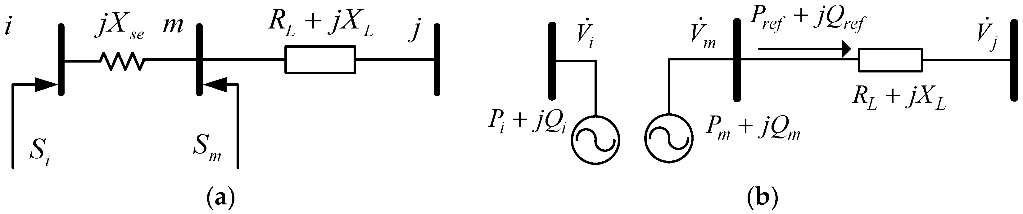
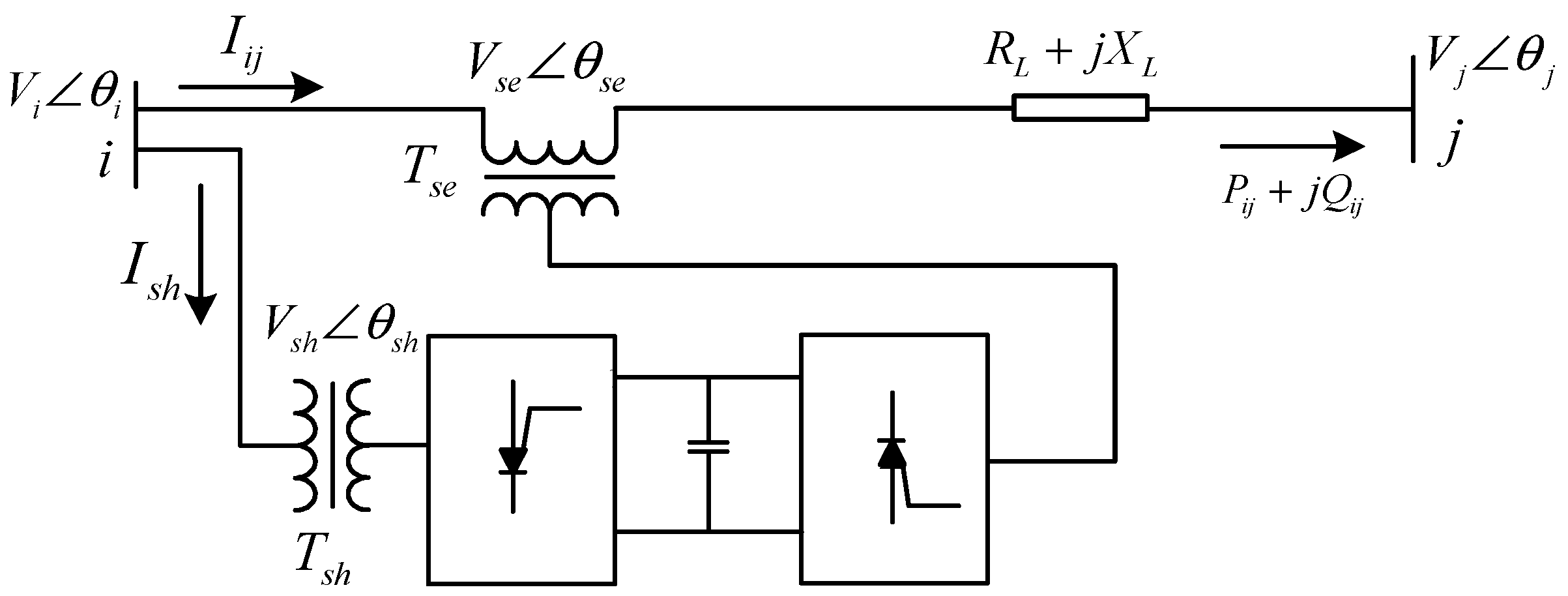
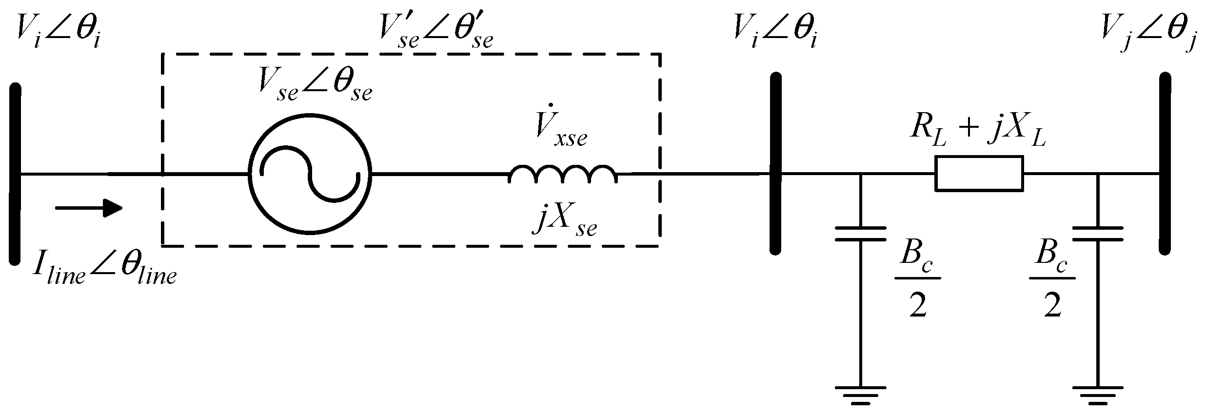
2. Power Flow Calculation with UPFC

2.1. Steady-State Model of UPFC

UPFC consists of two back-to-back converters, which are connected through the coupling capacitor, as shown in Figure 1.

At present, two kinds of steady-state model are mainly used to solve power flow calculation with UPFC, namely a power injection model and an additional node model [23,24], as shown in Figure 2. The control effect of UPFC is equivalent to the power injection in the power injection model and has been well-studied. For the UPFC additional node model, the input and output nodes of UPFC are equivalent to PV and PQ nodes, respectively, so that the power flow calculation with UPFC is transformed into the general power flow calculation, which could only be applied for UPFC to control the line power flow. The abovementioned two UPFC models will both be used in the following power flow calculation method, considering their own advantages and disadvantages.

2.2. Power Flow Calculation Method Considering UPFC Control Modes

The shunt side converter of UPFC is used in the automatic voltage control mode (which is normally used in practical applications) [21] in our paper. In this control mode, the shunt converter reactive current I_q is automatically regulated to maintain the line voltage to a reference value [21]. Therefore, node i connected to the shunt converter is considered as a PV node, and the injected reactive power Q_i can be obtained in power flow calculation. Then, the value of I_q can be calculated by I_q = Q_i/V_i.

The power flow control function of UPFC mainly depends on the series converter. The equivalent circuit of a UPFC series side inverter is shown in Figure 3. ${\dot{V}}_{se}$ is the output voltage of the UPFC series side inverter which removes the transformer reactance voltage drop, ${\dot{V}}_{xse}$ is the voltage drop generated by the transformer reactance of the UPFC series side inverter, and the ${\dot{V}}_{se}^{\prime }$ is the output voltage of the UPFC series side inverter. The power flow calculation method considering UPFC control modes will be deduced as follows.

2.2.1. Voltage Regulation Control Mode (VRCM)

The phase angle of the series inverter voltage is determined such that the phase angle is regulated in the same phase or the reversed phase of ${\dot{V}}_i$, and only the bus voltage amplitude of output side bus is adjusted. This control mode is called the voltage regulation control mode [21]. The power flow in voltage regulation control mode is calculated based on the UPFC power injection model. When the voltage of bus m is regulated to ${\dot{V}}_{ref}$, the voltage increment is calculated as follows:

$$\Delta \dot{V}={\dot{V}}_{ref}-{\dot{V}}_m$$

(1)

The voltage drop generated by the transformer reactance of the UPFC series side is given by:

$${\dot{V}}_{xse}=\left(\frac{{\dot{V}}_m-{\dot{V}}_j}{R_L+X_L}+{\dot{V}}_m·j\frac{B_c}{2}\right)·j{X}_{se}$$

(2)

Then, the iterative updating method of the UPFC series side control variables can be deduced by:

$$\Delta {\dot{V}}_{se}^{(k)}=\Delta {\dot{V}}^{(k)}+\Delta {\dot{V}}_{xse}^{(k)}$$

(3)

$${\dot{V}}_{se}^{(k+1)}={\dot{V}}_{se}{}^{(k)}+\Delta {\dot{V}}_{se}^{(k)}$$

(4)

where ${\dot{V}}_{se}$ is the output voltage of the UPFC series side inverter which removes the transformer reactance voltage drop, and the superscript $k$ is the iteration number of the power flow calculation. The $k+1$ time iterative value of the UPFC injection power can be calculated by Equations (1)–(4). The iterative calculation of the power flow will not stop until $\Delta V<\epsilon$.

2.2.2. Phase Regulation Control Mode (PRCM)

The mode where the voltage phase angle of ${\dot{V}}_m$ is kept at the desired value without changing the voltage amplitude is called the phase regulation control mode [21].

The UPFC power injection model is used to calculate the power flow in phase regulation control mode. If the phase angel of bus m is θ_m, the phase difference between bus m and bus i is θ_mi, which means: θ_mi = θ_m − θ_i. When the phase difference between bus m and bus i is controlled to θ_ref according to Figure 3, the following equations are obtained:

$$\Delta \theta ={\theta }_{ref}-{\theta }_{mi}$$

(5)

$$\Delta V_{se}^{\prime }=\sqrt{2}{V}_i·\sqrt{1-\cos (\Delta \theta )}$$

(6)

$$\Delta {\theta }_{se}^{\prime }=\frac{\Delta \theta }{2}+{(-1)}^n\frac{\pi }{2}$$

(7)

where $\Delta V_{se}^{\prime }$ and $\Delta {\theta }_{se}^{\prime }$ represent the increased voltage amplitude and the phase angle of the UPFC series side inverter containing the transformer voltage drop. When is $\Delta \theta$ less than zero, n = 1; when $\Delta \theta$ is equal to or greater than zero, n = 2.

Then, the iterative updating method of the UPFC series side control variables is deduced as follows:

$$\Delta {\dot{V}}_{se}^{(k)}=\Delta {{\dot{V}}^{\prime }}_{se}^{(k)}+\Delta {\dot{V}}_{xse}^{(k)}$$

(8)

$${\dot{V}}_{se}^{(k+1)}={\dot{V}}_{se}^{(k)}+\Delta {\dot{V}}_{se}^{(k)}$$

(9)

The k + 1 time UPFC injection power can be calculated by Equations (2) and (5)–(9). The power flow result is obtained when $\Delta \theta <\epsilon$.

2.2.3. Impedance Compensation Control Mode (ICCM)

The ratio of output voltage at the UPFC series side inverter to the line current is controlled to be constant so that UPFC will be regarded as a fixed impedance. This control mode of UPFC is called the impedance compensation control mode [21].

The UPFC power injection model is used to calculate the power flow in impedance compensation control mode. If the equivalent impedance between bus m and bus i is Z_mi and the desired equivalent impedance is Z_ref, the following equation can be obtained:

$${\dot{I}}_{mj}=\frac{{\dot{V}}_m-{\dot{V}}_j}{R_L+j{X}_L}+{\dot{V}}_m·j\frac{B_c}{2}$$

(10)

$$Z_{mi}=\frac{{\dot{V}}_m-{\dot{V}}_i}{{\dot{I}}_{mj}}$$

(11)

$$\Delta Z=Z_{ref}-Z_{mi}$$

(12)

The iterative updating method of the UPFC series side control variables is as follows:

$$\Delta {\dot{V}}_{se}^{\left(k\right)}=\Delta Z^{\left(k\right)}·{\dot{I}}_{mj}^{\left(k\right)}$$

(13)

$${\dot{V}}_{se}^{\left(k+1\right)}={\dot{V}}_{se}^{\left(k\right)}+\Delta {\dot{V}}_{se}^{\left(k\right)}$$

(14)

The k + 1 time UPFC injection power can be calculated by Equations (10)–(14). The power flow result is obtained until $\Delta Z<\epsilon$.

2.2.4. Constant Power Control Mode (CPCM)

The constant power control mode regulates the power flow of the target line to the required value [21]. In this mode, since the UPFC power injection model will slow down the power flow calculation speed, it is more appropriate to use the UPFC additional node model, as can be seen in Figure 2b. The specific power flow calculation process using the UPFC additional node model is presented as follows:

• The injection power of the PQ node is set to be equal to the reference power flow: $P_m+j{Q}_m=P_{ref}+j{Q}_{ref}$;
• The voltage of the PV node is set to be the reference voltage $V_i$. The injected active power of the PV node can be obtained according to active power balance between shunt and series converters of UPFC: $P_i=-P_m$;
• From this, the power flow is calculated, and all UPFC parameters are obtained.

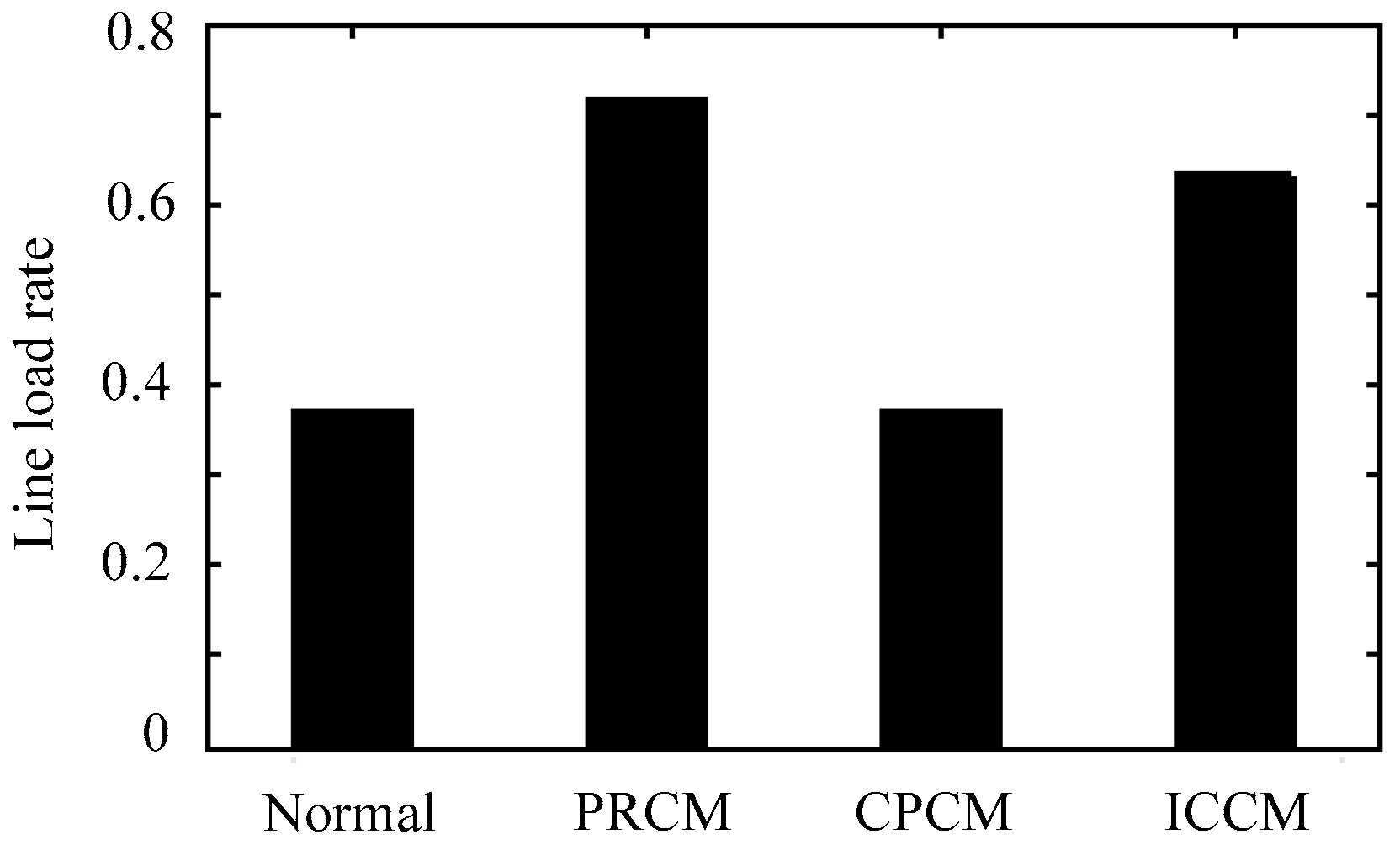
2.3. The Influence of UPFC Control Modes on System Static Security

Although all the four power flow control modes of UPFC can realize the adjustment of the power flow, they have different power flow control characteristics. In particular, when there are N-1 failures in the system, UPFC will response to the failures according to its control mode.

Numerical verification and analysis are carried out on the IEEE 30-bus test system. UPFC is installed on lines 4–6, and bus 31 corresponding to bus m in Figure 2 is added into the system for the convenience of description. The diagram of the IEEE 30-bus system is shown in Figure 4.

Taking CPCM, PRCM, and ICCM for instance, in order to compare the control difference among the three control modes after N-1 contingency, the initial power flow distribution of the three UPFC control modes should be the same. By testing the control target value shown in

Table 1. The control targets values of three control modes.

UPFC Control Mode	Value/p.u.
CPCM /Pref + jQref	−0.4774 + j0.0946
PRCM/θref	0.524
ICCM/Zref	0.0243 + j0.1037

, these three control modes obtain the same power flow result.

Lines 4–12 are chosen for the open circuit test, and the power flow after this contingency is calculated under different the UPFC control modes shown in Table 1. Taking lines 4–31 as an example, the load rate of lines 4–31 under normal state and these three UPFC control modes after contingency are shown in Figure 5.

As can be seen in Figure 5, the response of different control modes to N-1 contingency is inconsistent. The PRCM and ICCM enhance the load rate of lines 4–31 while the CPCM keeps the load rate unchanged under N-1 contingency. The above calculation results illustrate that different UPFC control modes can change the load rate when contingency occurs. Therefore, it is necessary to take UPFC control modes into consideration when checking the N-1 static security of the power system.

3. Preventive Security-Constrained Power Flow Optimization Including UPFC

3.1. Optimization Model

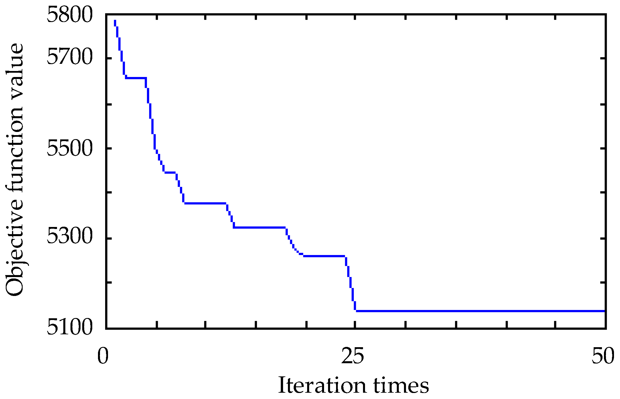
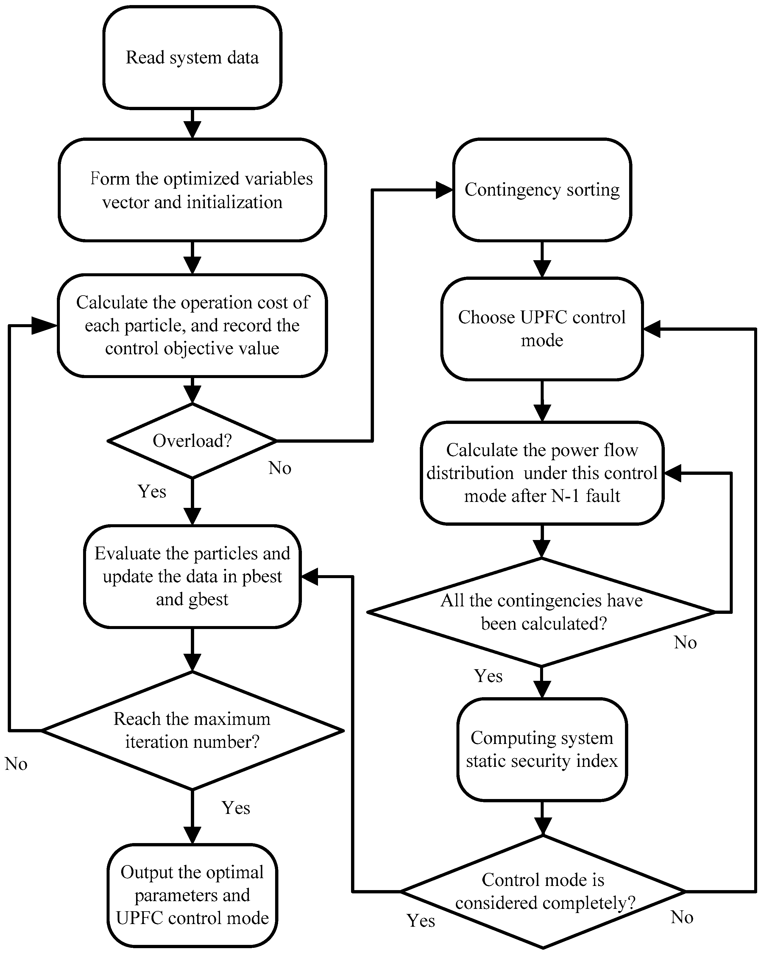
Taking the influence of different UPFC control modes on the distribution of power flow after N-1 fault into consideration, the optimization model is constructed as follows:

(1) The vector of control variable:

$$u=\left[V_G,P_G,T,C,\underset{UPFC}{\underbrace{V_{se},{\theta }_{se},I_q}}\right]$$

(15)

In (15), V_G and P_G are the voltage and active power of the generators. T is the position of the transformer tap. C is the capacity of the parallel compensation capacitor.

(2) Objective function:

$$F\left(x\right)={\omega }_{1}P\left(x\right)+{\omega }_2\left(N\left(x\right)+f\left(x\right)\right)r$$

(16)

The objective function can be divided into two parts: $P\left(x\right)$ and $N\left(x\right)r+f\left(x\right)$. In (17), $P\left(x\right)$ is used to represent the system operation cost, which can evaluate the economic efficiency of the system. Taking (18) to (21) for reference, $N\left(x\right)$ represents the maximum number of overloaded lines after N-1 contingency. $f\left(x\right)$ is the index of system static security. The smaller these two values are, the higher the static safety margin will be. Coefficient r is used to keep the system economics and static security index at the same magnitude. In this paper, r is equal to 10,000. ${\omega }_1$ and ${\omega }_2$ are weight coefficients.

$$P\left(x\right)={\displaystyle \sum _{i=1}^{N_g}\left(a_i{P}_{Gi}^2+b_i{P}_{Gi}+c_i\right)}+\eta P_{loss}$$

(17)

$$f\left(x\right)=1/d_{line}+d_{bus}$$

(18)

$$d_{line}=\Vert Q-LM\Vert =\sqrt{{\displaystyle \sum _{i=1}^n{\left(1-{\lambda }_i\right)}^2}}$$

(19)

$$d_{bus}=\sqrt{{\displaystyle \sum _{i=1}^k{\left(V_i-\overline{V}\right)}^2}}$$

(20)

$$\overline{V}=\frac{V_i^{\max }+V_i^{\min }}{2}$$

(21)

where a, b, c are generation cost coefficients, and $\eta$ is the price coefficient. $P_{loss}$ is the net active power loss. The adjustable range from operating point Q to the static safety limit LM is $d_{line}$, and the higher the value is, the stronger the static security will be. The rate of line load is $\lambda$. The distance between the bus voltage and the expectation value $\overline{V}$ is $d_{bus}$. The upper and lower bounds of the bus voltage are $V_i^{\max }$ and $V_i^{\min }$.

It should be noted that the influence of UPFC control modes is considered when calculating the static security margin index $f\left(x\right)$. By using the proposed method in Section 2.2, the power flow distribution under the four UPFC control modes after N-1 contingency can be obtained. Then, the static security margin index $f\left(x\right)$ of each control mode can be calculated through Equations (18)–(21). The minimal $f\left(x\right)$ is selected to determine the UPFC control mode and to calculate the objective function in Equation (16) for each feasible solution, and the objective function is used to determine the final optimal solution of the power flow optimization problem. The specific process is shown in Section 3.2.

(3) Equality constraints:

The power flow equality constraints are separated into two sets of active and reactive power balance equations, as follows:

$$\{\begin{array}{l}\Delta P_i=P_{Gi}-P_{Li}-V_i{\displaystyle \sum _{j=1}^N{V}_j\left(G_{ij}\cos {\theta }_{ij}+B_{ij}\sin {\theta }_{ij}\right)=0}\\ \Delta Q_i=Q_{Gi}-Q_{Li}-V_i{\displaystyle \sum _{j=1}^N{V}_j\left(G_{ij}\sin {\theta }_{ij}-B_{ij}\cos {\theta }_{ij}\right)=0}\end{array}$$

(22)

where $P_{Gi}$ and $Q_{Gi}$ are the generator real and reactive power at bus $i$, respectively. $P_{Li}$ and $Q_{Li}$ are the load real and reactive power at bus $i$, respectively. $G_{ij}$ and $B_{ij}$ are the real part and imaginary part of the admittance of lines $i-j$, respectively, and ${\theta }_{ij}={\theta }_i-{\theta }_j$.

By adding UPFC, the power balance equations will be changed as follows [19]:

$$\{\begin{array}{l}\Delta P_i=P_{Gi}-P_{Li}-V_i{\displaystyle \sum _{j=1}^N{V}_j\left(G_{ij}\cos {\theta }_{ij}+B_{ij}\sin {\theta }_{ij}\right)-P_{i\left(upfc\right)}=0}\\ \Delta Q_i=Q_{Gi}-Q_{Li}-V_i{\displaystyle \sum _{j=1}^N{V}_j\left(G_{ij}\sin {\theta }_{ij}-B_{ij}\cos {\theta }_{ij}\right)-Q_{i\left(upfc\right)}=0}\end{array}$$

(23)

where $P_{i\left(upfc\right)}$ and $Q_{i\left(upfc\right)}$ are the injected active and reactive powers by the FACTS device, respectively.

(4) Inequality constraints:

$$\{\begin{array}{l}{V}_{G\min }\le V_G\le V_{G\max }\\ P_{G\min }\le P_G\le P_{G\max }\\ T_{\min }\le T\le T_{G\max }\\ C_{\min }\le C\le C_{\max }\\ V_{se\min }\le V_{se}\le V_{se\max }\\ 0\le {\theta }_{se}\le 2\pi \\ i_{q\min }\le i_q\le i_{q\max }\end{array}$$

(24)

The constraints of the load node voltage, reactive power of the generators, and static security of the line, respectively, are as follows:

$$V_{\min }\le V\le V_{\max }$$

(25)

$$Q_{G\min }\le Q_G\le Q_{G\max }$$

(26)

$$P_i\le P_c$$

(27)

(5) Power flow constraints after contingency:

In addition to the above equality constraints and the inequality constraints, the static security constraints are included. If there are $N_c$ contingencies in the contingency set, the static security constraints can be represented as follows:

$$\{\begin{array}{l}{P}_1\left(c=1,2\cdots Nc\right)<P_{c1}\\ P_2\left(c=1,2\cdots Nc\right)<P_{c2}\\ ⋮\\ P_n\left(c=1,2\cdots Nc\right)<P_{cn}\end{array}$$

(28)

In (28), $P_1\left(c=1,2\cdots Nc\right)$ is the active power of line 1 after contingency occurs.

3.2. Model Solution

Based on the PSO algorithm, the specific solving progress shown in Figure 6 is as follows:

(1)

Input basic system data.

(2)

Set up the basic parameters of the PSO algorithm, and initialize the position and velocity vectors of each particle. The position information of particle includes system control parameters and UPFC control variables.

(3)

Calculate the power flow of each particle when the system is under normal state. Then, the system operation cost and the line overload condition are obtained. Meanwhile, the control objectives of each particle corresponding to four control modes are recorded.

(4)

Punish the particles with overload lines. The process of checking N-1 static security is conducted for the particles without overload lines according to the sorted contingency set. Then, the static security index corresponding to the four UPFC control modes after N-1 contingency continues being calculated until there is no overload phenomenon in three consecutive calculation results. By comparing the static safety indexes under the four UPFC control modes, the best UPFC control mode can be obtained.

(5)

Calculate the objective function, and obtain optimal individual and global solutions. Then, update the vectors of position and velocity of each particle.

(6)

Check whether the result has reached the maximum number of iterations. If not, turn to (3), else turn to (7).

(7)

Output the optimal results.

4. Case Studies

The IEEE 30-bus shown in Figure 4 is used as a case study to verify the effectiveness of the proposed method. UPFC is installed on lines 4–6, and the system reference power is 100 MVA. The upper and lower limit of the generator node voltage are 1.1 p.u. and 0.95 p.u. The transformer ratio ranges from 0.9 p.u. to 1.1 p.u., and the upper and lower gear number of transformers is ±5 by a step of 2%. The adjustable range of the two parallel capacitors is 0–0.5 p.u. and 0–0.1 p.u., and the step length is 0.1 p.u. and 0.02 p.u. respectively.

This paper modifies the thermal stability limit of some lines, and constructs a test system with static security problems. Based on the optimization process shown in Figure 6, the optimization program is written in MATLAB by using the particle swarm optimization (PSO) algorithm. The PSO parameters are as follows:

Inertia coefficient: w = 0.7298; acceleration coefficient: $c_1$ = 1.4962, $c_2$ = 1.4962; population size: POP = 50; maximum number of iteration: Num = 50. This example pays more attention to the static security of the system, and the weight coefficients are as follows: ${\omega }_1$ = 0.3, ${\omega }_2$ = 0.7.

The objective function values in each iteration are shown in Figure 7. The optimized control parameters of the system are given in

Table 2. The optimized system control parameters.

$V_2$	1.0484	$P_2$	0.365
$V_5$	1.0279	$P_5$	0.171
$V_8$	1.0253	$P_8$	0.482
$V_{11}$	1.0167	$P_{11}$	0.382
$V_{13}$	1.0449	$P_{13}$	0.149
$T_1$	1.06	$T_2$	0.92
$T_3$	0.96	$T_4$	0.94
$C_1$	0.2	$C_2$	0.06

. The UPFC control variables, control modes, and the corresponding control objective value are shown in

Table 3. The optimized parameters, control mode, and control objective value of UPFC.

${\mathit{V}}_{\mathit{s}\mathit{e}}$	${\mathit{\theta }}_{\mathit{s}\mathit{e}}$	${\mathit{V}}_6$	UPFC Control Mode	Control Objective Value
0.023	1.442	1.028	ICCM	−0.032 − j0.012

. The economy and static security of the system are compared in

Table 4. The comparison of system economic efficiency and static security index before and after optimization.

	System Operation Cost/$	The Number of Overloaded Lines (Normal)	The Number of Overloaded Lines (N-1)	Index of Static Security Margin
Before	10652	1	4	0.37
After	9755	0	0	0.31

.

As can be seen in Table 4, the cost of the testing system has been greatly reduced through the optimization algorithm proposed in this paper. As for static security, there are obvious static security problems in the original system. The overload phenomenon emerges in both the normal and N-1 situation. After optimization by using the proposed method, the overload phenomenon disappears. Meanwhile, according to (18) to (21), the lower the index of static security margin is, the higher the system static security margin will be. Compared with the initial static security margin index, the optimized static security margin index significantly decreases. Therefore, this method is feasible and effective to guarantee and improve the static security of the power system.

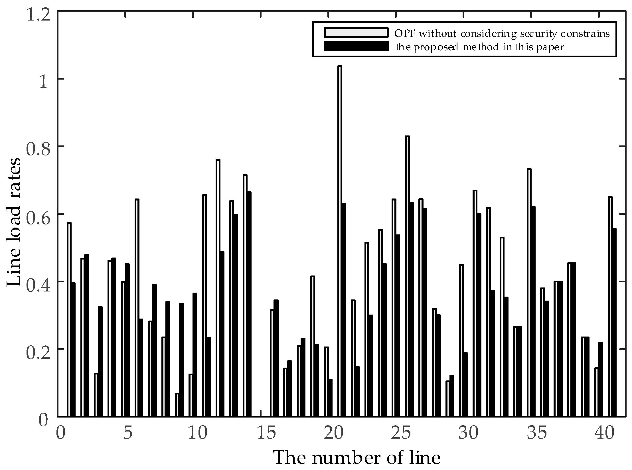
5. Comparison with Two Existing Optimization Methods

To further verify the advantages of the proposed preventive security-constrained power flow optimization method considering UPFC control modes, the proposed method in this paper is compared to two existing optimization methods as follows:

(1)

Optimal power flow without considering security constrains, as in Reference [5]

(2)

Preventive security-constrained optimal power flow only considering a fixed UPFC control mode, as in Reference [20].

5.1. Case A: Optimal Power Flow Without Considering Security Constrains

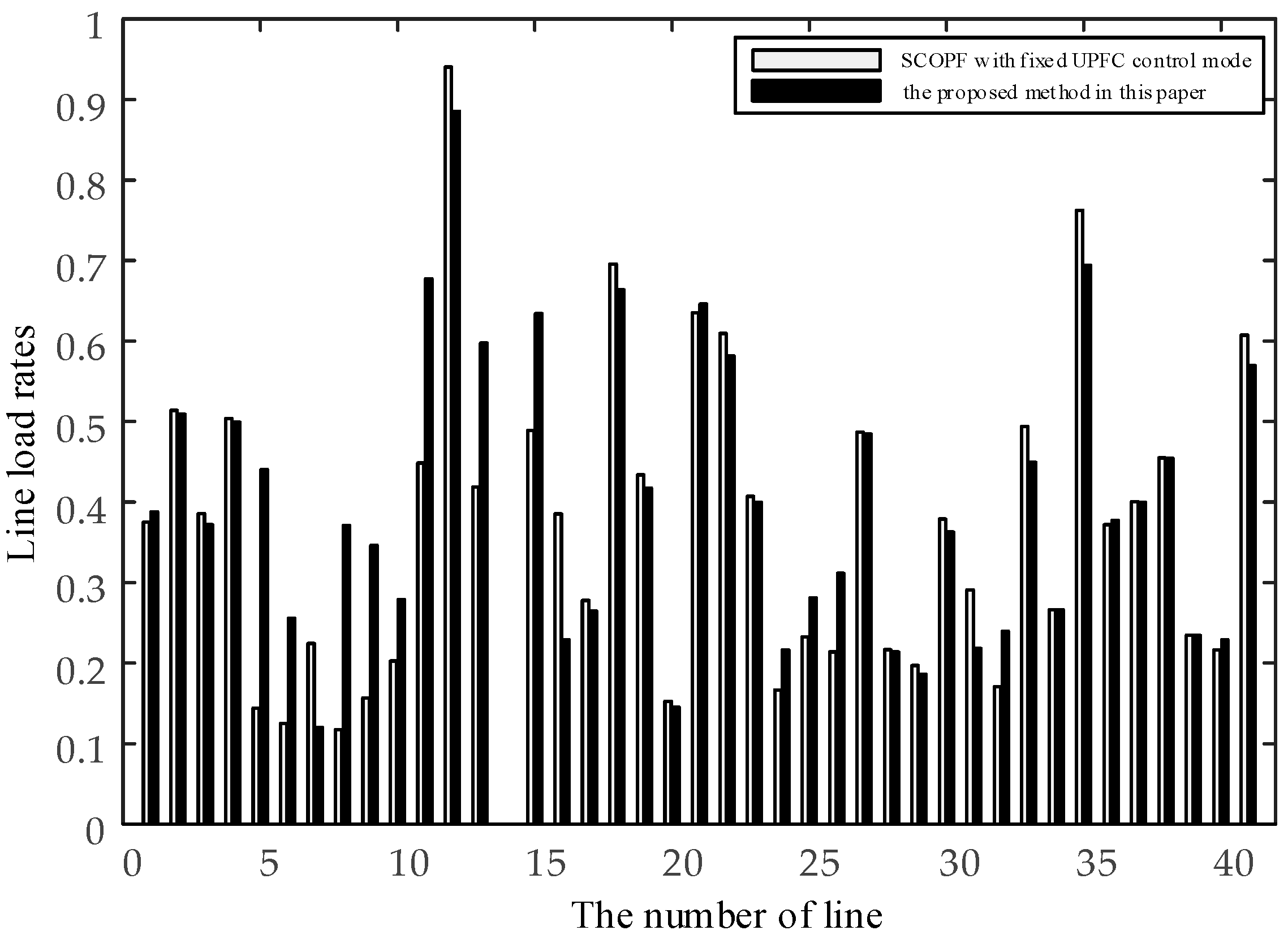
The objective function is:

$$F\left(x\right)={\displaystyle \sum _{i=1}^{N_g}\left(a_i{P}_{Gi}^2+b_i{P}_{Gi}+c_i\right)}+\eta P_{loss}$$

(29)

where $F\left(x\right)$ represents the system operation cost, same as Equation (17).

The initial operating parameters of the system and the parameters of the PSO algorithm are consistent with Section 4. The optimized results without considering security constrains are shown in

Table 5. The optimized system control parameters in Case A.

$V_2$	1.0472	$P_2$	0.059
$V_5$	1.0281	$P_5$	0.782
$V_8$	1.0219	$P_8$	0.365
$V_{11}$	0.9854	$P_{11}$	0.272
$V_{13}$	1.0512	$P_{13}$	0.247
$T_1$	1.020	$T_2$	1
$T_3$	0.98	$T_4$	0.96
$C_1$	0.2	$C_2$	0.08
$V_{se}$	0.008	${\theta }_{se}$	6.099
$V_6$	1.057

and

Table 6. The comparison of system economic efficiency and static security index before and after optimization in Case A.

	System Operation Cost/$	The Number of Overloaded Lines (Normal)	The Number of Overloaded Lines (N-1)	Index of Static Security Margin
Before	10652	1	4	0.37
After	9679	0	1	0.35

.

Comparing the operation cost after optimization in Table 6 and Table 4, the economy is improved in Case A. However, there is still one line overloaded for N-1 contingency after optimization, which is not allowed for practical operation. Under the failure of lines 4–12, the load rates obtained by the OPF with and without considering security constrain are compared in Figure 8. As can be seen in Figure 8, line No. 21 (corresponding to lines 16–17 in Figure 4) is overloaded, which means that the optimized operating condition obtained by the proposed method is better.

5.2. Case B

The preventive security-constrained optimal power flow is obtained only considering the constant power control mode of UPFC. The objective function, the initial operating parameters of the system, and the parameters of the PSO algorithm are the same as in Section 4. The optimized results are shown in

Table 7. The optimized system control parameters in Case B.

$V_2$	1.0338	$P_2$	0.059
$V_5$	1.0264	$P_5$	0.782
$V_8$	1.0279	$P_8$	0.365
$V_{11}$	1.0316	$P_{11}$	0.272
$V_{13}$	1.0295	$P_{13}$	0.247
$T_1$	1	$T_2$	1
$T_3$	0.94	$T_4$	0.94
$C_1$	0.3	$C_2$	0.08

,

Table 8. The optimized parameters, control mode, and control objective value of UPFC in Case B.

${\mathit{V}}_{\mathit{s}\mathit{e}}$	${\mathit{\theta }}_{\mathit{s}\mathit{e}}$	${\mathit{V}}_6$	UPFC Control Mode	Control Objective Value
0.008	5.281	1.030	CPCM	−0.254 + j0.140

and

Table 9. The comparison of system economic efficiency and static security index before and after optimization in Case B.

	System Operation Cost/$	The Number of Overloaded Lines (Normal)	The Number of Overloaded Lines (N-1)	Index of Static Security Margin
Before	10652	1	4	0.37
After	9812	0	0	0.33

.

Comparing the results between Table 4 and Table 9, when the UPFC control mode is fixed in constant power control mode, the operation cost and the static security of the system are also optimized, but the operation cost is higher only considering the constant power control mode of UPFC. In addition, the static security margin index in constant power control mode is higher than that considering all UPFC control modes, which means that the optimization of the UPFC control mode is effective and necessary to improve the static security of the power system.

Under the failure of lines 9–10, the load rates obtained by SCOPF with and without considering the UPFC control mode are compared in Figure 9. As can be seen in Figure 9, the load rate of line No. 12 and line No. 35 (corresponding to lines 6–10 and lines 25–27 in Figure 4) are higher without considering UPFC control modes, indicating that the optimized operating condition obtained by the proposed method is better.

6. Conclusions

Based on the UPFC power injection model and additional node model, an iterative method for power flow calculation considering UPFC control modes is deduced. Moreover, it is proven that the power flow control mode of UPFC affects the static security of the power system.

A preventive security-constrained power flow optimization model considering UPFC control modes is established. The proposed model integrates the economic efficiency and static security of the power system, and constructs the corresponding objective function. Furthermore, the influence of the UPFC control modes on power system static security is incorporated into the power flow optimization, and the UPFC control mode is selected in each iteration. Through solving the proposed model, the system control parameters, UPFC optimal control mode, and control target value can be obtained simultaneously. The calculation results in the testing system show that the proposed method is feasible and effective.

References

1. Albatsh, F.M.; Mekhilef, S.; Ahmad, S.; Mokhlis, H. Fuzzy Logic Based UPFC and Laboratory Prototype Validation for Dynamic Power Flow Control in Transmission Line. IEEE Trans. Ind. Electron. 2017. [Google Scholar] [CrossRef]
2. Chivite-Zabalza, J.; Rodriguez Vidal, M.A.; Izurza-Moreno, P.; Calvo, G.; Madariaga, D. A Large-Power Voltage Source Converter for FACTS Applications Combining Three-Level Neutral-Point-Clamped Power Electronic Building Blocks. IEEE Trans. Ind. Electron. 2013, 60, 4759–4772. [Google Scholar] [CrossRef]
3. Golshannavaz, S.; Aminifar, F.; Nazarpour, D. Application of UPFC to Enhancing Oscillatory Response of Series-Compensated Wind Farm Integrations. IEEE Trans. Smart Grid 2014, 5, 1961–1968. [Google Scholar] [CrossRef]
4. Monteiro, J.; Pinto, S.; Martin, A.D.; Silva, J.F. A New Real Time Lyapunov Based Controller for Power Quality Improvement in Unified Power Flow Controllers Using Direct Matrix Converters. Energies 2017, 10, 779. [Google Scholar] [CrossRef]
5. Venkateswara Rao, B.; Nagesh Kumar, G.V. Optimal power flow by BAT search algorithm for generation reallocation with unified power flow controller. Int. J. Electr. Power Energy Syst. 2015, 68, 81–88. [Google Scholar] [CrossRef]
6. Reddy K, A.K.; Singh, S.P. Congestion mitigation using UPFC. IET Gener. Transm. Distrib. 2016, 10, 2433–2442. [Google Scholar]
7. Rajabi-Ghahnavieh, A.; Fotuhi-Firuzabad, M.; Othman, M. Optimal unified power flow controller application to enhance total transfer capability. IET Gener. Transm. Distrib. 2015, 9, 358–368. [Google Scholar] [CrossRef]
8. Sarker, J.; Goswami, S.K. Solution of multiple UPFC placement problems using Gravitational Search Algorithm. Int. J. Electr. Power Energy Syst. 2014, 2, 531–541. [Google Scholar] [CrossRef]
9. Bhattacharyya, B.; Kumar, S. Approach for the solution of transmission congestion with multi-type FACTS devices. IET Gener. Transm. Distrib. 2016, 10, 2802–2809. [Google Scholar] [CrossRef]
10. Ren, B.X.; Cai, H.; Du, W.J.; Wang, H.F.; Fan, L.L. Analysis of Power Flow Control Capability of a Unified Power Flow Controller to be installed in a Real Chinese Power Network. In Proceedings of the 12th IET International Conference on AC and DC Power Transmission, Beijing, China, 28–29 May 2016. [Google Scholar]
11. Sass, F.; Sennewald, T.; Marten, A.K.; Westermann, D. Mixed AC high-voltage direct current benchmark test system for security constrained optimal power flow calculation. IET Gener. Transm. Distrib. 2017, 2, 447–455. [Google Scholar] [CrossRef]
12. Goldis, E.A.; Ruiz, P.A.; Caramanis, M.C.; Li, X.; Russ Philbrick, C.; Rudkevich, A.M. Shift Factor-Based SCOPF Topology Control MIP Formulations With Substation Configurations. IEEE Trans. Power Syst. 2017, 2, 1179–1190. [Google Scholar] [CrossRef]
13. An, K.; Song, K.B.; Hur, K. Incorporating Charging/Discharging Strategy of Electric Vehicles into Security-Constrained Optimal Power Flow to Support High Renewable Penetration. Energies 2017, 10, 729. [Google Scholar] [CrossRef]
14. Thomas, J.J.; Grijalva, S. Flexible Security-Constrained Optimal Power Flow. IEEE Trans. Power Syst. 2015, 3, 1195–1202. [Google Scholar] [CrossRef]
15. Phan, D.T.; Sun, X.A. Minimal Impact Corrective Actions in Security-Constrained Optimal Power Flow via Sparsity Regularization. IEEE Trans. Power Syst. 2015, 30, 1947–1956. [Google Scholar] [CrossRef]
16. Kaur, M.; Dixit, A. Newton’s Method approach for Security Constrained OPF using TCSC. In Proceedings of the IEEE 1st International Conference on Power Electronics, Intelligent Control and Energy Systems, Delhi, India, 4–6 July 2016. [Google Scholar]
17. Shchetinin, D.; Hug, G. Decomposed algorithm for risk-constrained AC OPF with corrective control by series FACTS devices. Electr. Power Syst. Res. 2016, 141, 344–353. [Google Scholar] [CrossRef]
18. Babu, A.V.N.; Sivanagaraju, S. Optimal power flow with FACTS device using two step initialization based algorithm for security enhancement considering credible contingencies. In Proceedings of the International Conference on Advances in Power Conversion and Energy Technologies, Mylavaram, Andhra Pradesh, India, 2–4 August 2012. [Google Scholar]
19. Ara, A.L.; Aghaei, J.; Alaleh, M.; Barati, H. Contingency-based optimal placement of Optimal Unified Power Flow Controller (OUPFC) in electrical energy transmission systems. Sci. Iran. 2013, 3, 778–785. [Google Scholar]
20. Kumar, G.N.; Kalavathi, M.S. Cat Swarm Optimization for optimal placement of multiple UPFC’s in voltage stability enhancement under contingency. Int. J. Electr. Power Energy Syst. 2014, 57, 97–104. [Google Scholar] [CrossRef]
21. Eremia, M.; Liu, C.C.; Edris, A.A. Advanced Solutions in Power Systems: HVDC, FACTS, and Artificial Intelligence; John Wiley & Sons: New Jersey, NJ, USA, 2016; pp. 579–581. [Google Scholar]
22. Chandana, D.; Marutheswar, G.V. Power Quality Enhancement in a Transmission Line using UPFC based on Fuzzy Logic Controller. Int. J. Recent Technol. Mech. Electr. Eng. 2015, 10, 27–31. [Google Scholar]
23. Pereira, M.; Cera Zanetta, L. A current based model for load flow studies with UPFC. IEEE Trans. Power Syst. 2013, 28, 677–682. [Google Scholar] [CrossRef]
24. Bhowmick, S.; Das, B.; Kumar, N. An indirect upfc model to enhance reusability of newton power-flow codes. IEEE Trans. Power Deliv. 2008, 23, 2079–2088. [Google Scholar] [CrossRef]
Figure 1. Per-phase schematic diagram of unified power flow controller (UPFC).
Energies 10 01199 g001
Figure 2. The power flow calculation model of UPFC: (a) power injection model of UPFC; (b) additional node model of UPFC.
Energies 10 01199 g002
Figure 3. The equivalent circuit of UPFC series side.
Energies 10 01199 g003
Figure 4. Diagram of IEEE 30-bus system.
Energies 10 01199 g004
Figure 5. Load rates of lines 4–31.
Energies 10 01199 g005
Figure 6. The flowchart of power flow optimization with UPFC control modes.
Energies 10 01199 g006
Figure 7. The objective function value vs. iteration times.
Energies 10 01199 g007
Figure 8. The comparison of line load rate under the failure of lines 4–12.
Energies 10 01199 g008
Figure 9. The comparison of line load rate under the failure of lines 9–10.
Energies 10 01199 g009