A Comparative Study of Three Improved Algorithms Based on Particle Filter Algorithms in SOC Estimation of Lithium Ion Batteries

Abstract

The state of charge (SOC) is an important parameter for batteries, especially those for electric vehicles. Since SOC cannot be obtained directly by measurement, SOC estimation methods are required. In this paper, three model-based methods, including the extended particle filter (EPF), cubature particle filter (CPF), and unscented particle filter (UPF), are compared in terms of complexity, accuracy, and robustness. The second-order resistor-capacitor (RC) equivalent circuit model is selected as the circuit model of the lithium-ion battery, and the parameters of the model are obtained by off-line identification. Then, the City test is applied to compare the performance of the methods. The experimental results show that the EPF method exhibits low complexity and fast running speed, but poor accuracy and robustness. Compared with the EPF method, the complexity of the CPF and UPF methods is relatively high, but these models offer improved accuracy and robustness.

1. Introduction

Lithium-ion batteries have advantages of high energy density, low self-discharge rate, and long cycle life, leading to their wide usage in electric vehicles and other electric storage devices. However, lithium-ion batteries also have shortcomings, such as the requirement for a special protection circuit—a battery management system (BMS)—to prevent battery overcharge and over-discharge, and to protect the normal function. State of charge (SOC) indicates the battery power situation, and SOC estimation is an important function of a BMS. An accurate SOC assessment is required to maximize the performance of lithium-ion batteries. For electric vehicles, SOC estimation is used to estimate the remaining mileage of electric vehicles, allowing the driver to reasonably plan their travel. Unlike our daily measurement of the length or weight of an object, for example, SOC cannot be directly measured. Further, the SOC cannot be calculated by a simple calculation, but must be obtained by specific estimation methods based on the voltage and current, temperature, and other conditional information containing noise.

Many SOC estimation methods have been proposed, but these algorithms have certain shortcomings, and no single algorithm provides the best performance for all situations. According to the SOC definition, the Ampere-hour integral method [1,2,3] integrates the battery charge and discharges current and adds it to the initial SOC value to obtain the SOC value. This algorithm does not need to establish a model of the battery, and it is simple and easy to implement. However, in the actual work process, the current measured by the sensor may be inaccurate, and the initial SOC cannot be obtained accurately, so there is a cumulative error as the method is used, and this error of SOC cannot be corrected. The open circuit voltage method [4] also does not require establishment of a battery model; the relationship between the open circuit voltage and SOC is determined experimentally, and then the SOC value is obtained according to the battery open circuit voltage. However, the open-circuit voltage of the battery is difficult to obtain, so this method is not suitable for practical SOC estimation. The artificial neural network method also does not need a battery model, but requires a lot of data to be used for algorithm training, and the estimation accuracy is highly dependent on the quality and quantity of the training data.

The Kalman filter (KF) is a model-based and closed-loop method based on a battery model, and offers higher estimation accuracy than non-model-based methods and can be self-corrected. The KF algorithm requires a linear battery model, although battery models are generally non-linear. In order to allow the KF method to adapt to the nonlinear problem, the EKF method [5,6,7], the CKF method [8,9,10], and the UKF method [11,12] are proposed in succession. The EKF method linearizes the nonlinear system, which introduces a linearization error, resulting in deterioration of the state estimation accuracy. The CKF uses the radial-spherical cubature rule to approximate the states of a non-linear system with additive Gaussian noise. The UKF method reduces the error caused by linearization of the EKF and improves the estimation accuracy through UT transformation. Particle filtering (PF) [13,14] is a Bayesian estimation method based on Monte Carlo simulation using a series of weighted random sampling particles to approximate the probability distribution function (PDF). It is independent of the system model and is not subject to linearization error or Gaussian noise assumption. It can solve the error caused by the linearization of EKF and avoid the error caused by the non-Gaussian PDF. It is suitable for any environment, and any state model and observation model. Due to the deviation between the importance function and the true posterior probability, the general effect of particle filter estimation is not ideal.

The KF method combined with the PF method not only improves the robustness of the KF algorithm, but also solves the difficulty of PDF selection of the PF algorithm. The EKF, CKF, and UKF methods, three classical improved methods for the KF algorithm, which are compared in detail in [9,13,15], are also improved when combined with the PF method. The extended particle filter (EPF) method, based on the EKF method and the PF method, has been applied in other research areas and has not been used in SOC estimation [16,17,18]. The cubature particle filter (CPF) method combined with the CKF and the PF methods has a greater advantage over both methods [19,20]. Similarly, the unscented particle filter (UPF) method is derived from the combination of the UKF and the PF methods [21,22]. In this study, the City condition test was used to test the SOC estimation accuracy of the EPF, CPF, UPF methods and the run time of the process was calculated for each method to compare model complexity. The initial SOC value is set to the real initial SOC value, and the SOC estimation accuracy for the three methods at different times are determined, thus comparing the convergence speed of the methods. Finally, noise was added to the City condition to compare the robustness of the methods.

The remaining parts of this paper are organized as follows: In Section 2, the second-order model of the battery is described and the parameters are identified. Section 3 mainly introduces the flow of the three methods. The detailed description of the various required experimental equipment and the comparison of the performance of the methods are described in Section 4. Section 5 presents the conclusions of the paper.

2. Battery Modeling and Parameters Identification

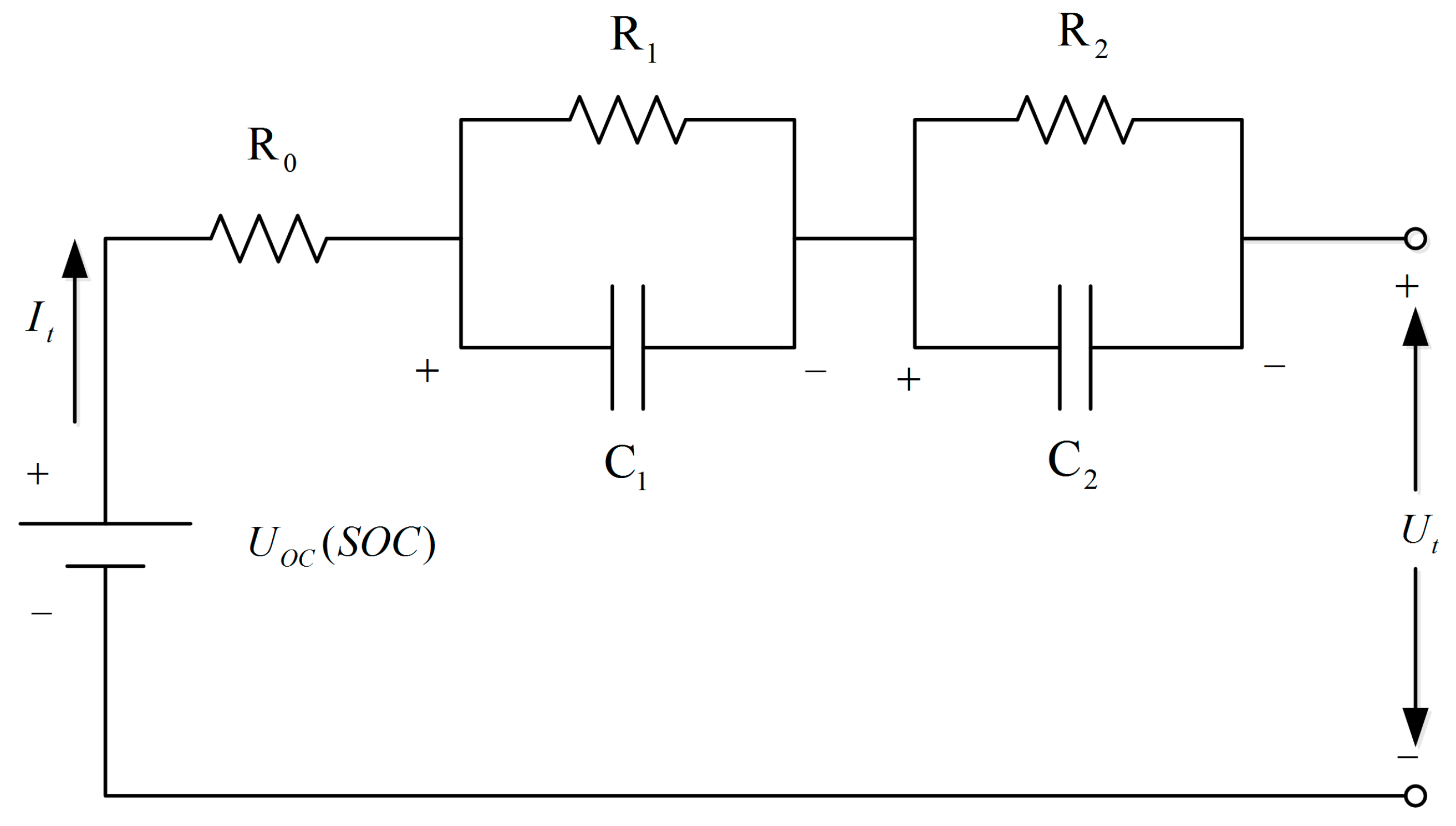
2.1. The SOC Definition and the Battery Model

SOC reflects the capacity remaining state of the battery, which is usually defined as the ratio of the remaining capacity of the battery to the rated capacity. According to the definition of SOC, Equation (1) can be obtained as follows:

$$SOC(t)=SOC(t_0)-\frac{{\displaystyle {\int }_{t_0}^{t}idt}}{Q_N}$$

(1)

Equation (2) is the derivation of Equation (1):

$$\dot{SOC}(t)=-\frac{i(t)}{Q_N}$$

(2)

where $SOC(t_0)$ and $SOC(t)$ denote the SOC values at time $t_0$ and $t$, respectively. $i$ represents the current during charging and discharging, and the current is negative at the time of charging and positive when discharging. $Q_N$ represents the rated capacity of the battery.

The EPF method, the CPF method, and the UPF method are all model-based methods. The battery model reflects the charge and discharge characteristics of the battery, providing a basis for SOC estimation. Previous studies have proposed many models such as the equivalent circuit model [23,24,25], the electrochemical model [26], the electrical thermal model [27], and others. The equivalent circuit model is widely used in the SOC estimation of lithium ion batteries. The second-order equivalent circuit model has higher accuracy than the first-order equivalent circuit model, and smaller computational complexity than other high-order circuit models [28]. Therefore, the second-order equivalent circuit model was applied in this study for SOC estimation. As shown in Figure 1, the second-order equivalent circuit model consists of an open circuit voltage $U_{OC}(SOC)$ that changes with the SOC value, a resistor $R_0$ and two $RC$ networks. The resistor $R_0$ is the ohmic resistance, $R_1$ and $C_1$ are the activation polarization resistance and the polarization capacitance, respectively, and $R_2$ and $C_2$, respectively, are the concentration polarization resistance and the polarization capacitance.

According to the second-order equivalent circuit model shown in Figure 1, the following three equations can be obtained:

$$\dot{U_1}=\frac{1}{C_1}i(t)-\frac{1}{C_1{R}_1}{U}_1$$

(3)

$$\dot{U_2}=\frac{1}{C_2}i(t)-\frac{1}{C_2{R}_2}{U}_2$$

(4)

$$U_t=U_{oc}(SOC)-U_1-U_2-R_{0}i(t)$$

(5)

where $U_1$ and $U_2$ denote the terminal voltages of the $R_1{C}_1$ and $R_2{C}_2$ networks, respectively. $\dot{U_1}$ and $\dot{U_2}$ represent the derivatives of $U_1$ and $U_2$, respectively.

Consider the current $i(t)$ as the model input $u$ and the voltage $U_t$ as the model output $y$. Combine Equations (2)–(4) and select $x={[SOC,U_1,U_2]}^{\mathrm{T}}$ as the state vector, and then the discrete-time state space equations can be deduced as:

$$\left(\begin{array}{c}SOC(k)\\ U_1(k)\\ U_2(k)\end{array}\right)=\left(\begin{array}{ccc}1& 0& 0\\ 0& 1-\frac{T}{C_1{R}_1}& 0\\ 0& 0& 1-\frac{T}{C_2{R}_2}\end{array}\right)\left(\begin{array}{c}SOC(k-1)\\ U_1(k-1)\\ U_2(k-1)\end{array}\right)+\left(\begin{array}{c}-\frac{T}{Q_N}\\ \frac{T}{C_1}\\ \frac{T}{C_2}\end{array}\right)i(k)$$

(6)

$$U_t(k)=U_{oc}(SOC)-R_{0}i(k)-U_1(k)-U_2(k)$$

(7)

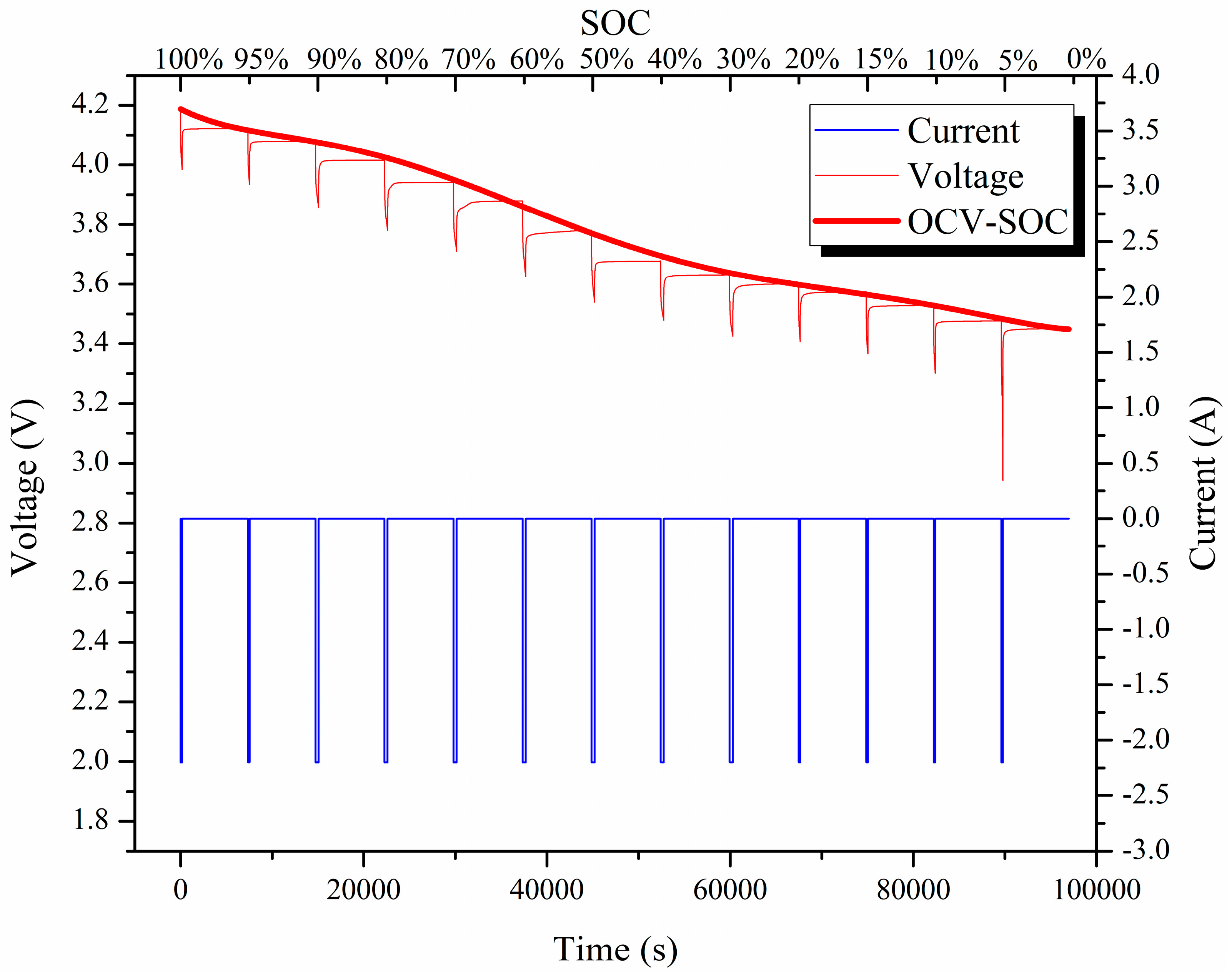
2.2. Parameter Identification

According to the second-order RC equivalent circuit model established in Figure 1, to further estimate the SOC value, we must first determine the parameters $R_0$, $R_1$, $R_2$, $C_1$, and $C_2$, and the corresponding relationship between the open circuit voltage and SOC. The following experiments were carried out using Samsung ICR18650-22P lithium-ion batteries, and the detailed description of the experimental equipment is provided in Section 4. The experiment procedure was performed as follows: (1) The constant current constant voltage (CCCV) method was used to charge the battery to an upper limit cut-off voltage of 4.2 V, and then set aside for 2 h. Next, the battery was discharged to the lower limit cut-off voltage of 2.75 V at 1 C, and then set aside for 2 h; (2) Step (1) was performed three times, using the average of the three discharges (1.98 Ah) as the actual capacity of the battery; (3) Finally, 1 C discharge was done to 90%, 80%, 70%, 60%, 50%, 40%, 30%, 20%, 15%, 10%, 5%, and 0% of the battery capacity, and then stopped for 2 h after each discharge.

The performance of the battery is supposed to change during the charging-discharging process and the aging process. Therefore, when the second-order RC equivalent circuit is used as the battery model, parameters $R_0$, $R_1$, $R_2$, $C_1$, and $C_2$ will also change in the battery charging-discharging process and aging process. There is no doubt that online parameter identification of these parameters is more helpful in improving model veracity and SOC estimation accuracy. However, it is beyond the scope of this paper. The offline identification method is used in this paper. In the above experiment, a discharge and static process was selected for parameter identification and the first section of the discharge and static curve has been selected (in fact, the selection of which section has little effect on the estimation accuracy). The widely-used exponential function fitting method is used to identify the parameters $R_0$, $R_1$, $R_2$, $C_1$, and $C_2$, which are identified as follows:

$$R_0=0.0377,R_1=0.0242,R_2=0.0030,C_1=1673.3,C_2=178230.$$

The experimental results are shown in Figure 2. The abscissa indicates the discharge time of the battery, and each time period corresponds to a different SOC value. The blue solid line and the red solid line indicate the battery discharge current and battery voltage curve with time, respectively. The red thick solid line in Figure 2 represents the correspondence between the open circuit voltage (OCV) and the SOC obtained by the sixth order polynomial fitting.

$$U_{OC}(SOC)=12.26SO{C}^6-28.81SO{C}^5+20.72SO{C}^4-2.60SO{C}^3-1.91SO{C}^2+1.08SO{C}^1+3.44$$

(8)

3. Algorithm Flow

3.1. Extended Particle Filter (EPF)

• Initialize particles:

  $$x_0^i~p(x_0),{\widehat{P}}_0^i=\mathrm{var}(x_0),w_0^i=\frac{1}{N}$$

  (9)

  where $x_0^i$ represents the initial state of the i-th particle and ${\widehat{P}}_0^i$ represents the initial error covariance of the i-th particle. $w_0^i$ is the initial weight of the i-th particle and $N$ indicates the total number of particles. Additionally, the article selects N = 50 as an example.
• Predict the state and the error covariance:

  $$x_{k|k-1}^i=f(x_{k-1}^i)$$

  (10)

  $$P_{k|k-1}^i=F_k^i{P}_{k-1}{(F_k^i)}^{\mathrm{T}}+F_k^i{Q}_k{(F_k^i)}^{\mathrm{T}}$$

  (11)

  where $Q_k$ is the process noise covariance at time k. $F_k^i$ is the process matrix.
• Calculate the Kalman gain:

  $$K=P_{k|k-1}^i{H}_k^i{[U_k^i{R}_k{(U_k^i)}^{\mathrm{T}}+H_k^i{P}_{k|k-1}^i{(H_k^i)}^{\mathrm{T}}]}^{-1}$$

  (12)

  where $R_k$ denotes the measurement noise covariance at time k. $H_k^i$ is the measure matrix.
• Update the predicted state and the error covariance:

  $${\widehat{x}}_k^i={\widehat{x}}_{k|k-1}^i+K(y_k^i-h({\widehat{x}}_{k|k-1}^i))$$

  (13)

  $${\widehat{P}}_k^i=P_{k|k-1}^i-K{H}_k^i{P}_{k|k-1}^i$$

  (14)
• Update particles:

  $$x_k^i~q({\widehat{x}}_k^i|x_{k-1}^i,y_k^i)=N({\widehat{x}}_k^i,{\widehat{P}}_k^i)$$

  (15)
• Calculate the weights of the particles:

  $$w_k^i=w_{k-1}^i\frac{p(y_k|{\widehat{x}}_k^i)p({\widehat{x}}_k^i|x_{k-1}^i)}{q({\widehat{x}}_k^i|x_{k-1}^i,y_{1:k})}$$

  (16)
• Normalize weights:

  $$w_k^i=w_k^i{({\displaystyle \sum _{j=1}^N{w}_k^j})}^{-1}$$

  (17)
• Resampling:

A detailed description of resampling is in [29].

The selection of Q, R requires a certain assessment of working conditions and noise environment. The estimation accuracy will be improved if the selection of Q, R is accurate and suitable enough. It is fairly difficult to exactly assess working conditions and noise environment for practical application. Some research imports adaptive algorithms to constantly revise the values of Q and R. However, this is beyond the research scope of this paper. In this paper, Q and R are selected based on a ballpark assessment of practical working conditions, with the purpose of comparing the performance of different algorithms. During the comparison, the values of Q and R as follows are the same in different algorithms:

$$Q=\left\{\begin{array}{ccc}{10}^{-3}& 0& 0\\ 0& {10}^{-4}& 0\\ 0& 0& {10}^{-4}\end{array}\right\},R=\left\{{10}^{-2}\right\}$$

Moreover, H and P are constantly updated in the computation process of algorithms.

3.2. Cubature Particle Filter (CPF)

• Initialize particles:

  $$x_0^i~p(x_0),{\widehat{P}}_0^i=\mathrm{var}(x_0),w_0^i=\frac{1}{N}$$

  (18)
• Calculate the cubature points for each particle:

  $$P_{k-1|k-1}^i=S_{k-1|k-1}^i{(S_{k-1|k-1}^i)}^{\mathrm{T}}$$

  (19)

  $$C_{j,k}=S_k{\xi }_i+{\widehat{x}}_k\hspace{1em}i=1,2,\cdots ,2n$$

  (20)

  $${\xi }_j=\sqrt{n}{[1]}_j\hspace{1em}j=1,\cdots ,2n$$

  (21)
  ${[1]}_j$ denotes that the point is centered at the j-th point of $[1]$, and the symbol $[1]$ is a complete set of all symmetric points, denoting the set of points generated by the full permutation of the elements of the n-dimensional unit vector $e={[1,0,\cdots ,0]}^{\mathrm{T}}$ and the change of the element symbol.
• Propagate the cubature points and calculate the predicted state:

  $$x_{k|k-1}^{i,(c)}=f(C_{j,k},u_k)$$

  (22)

  $${\widehat{x}}_{k|k-1}^i=\frac{1}{2n}{\displaystyle \sum _{c=1}^{2n}{x}_{k|k-1}^{i,(c)}}$$

  (23)

  $$P_{k|k-1}=\frac{1}{2n}{\displaystyle \sum _{c=1}^{2n}{(x_{k|k-1}^{i,(c)})}^{\mathrm{T}}(x_{k|k-1}^{i,(c)})-{\widehat{x}}_{k|k-1}^i{({\widehat{x}}_{k|k-1}^i)}^{\mathrm{T}}+Q_k}$$

  (24)
• Calculate the cubature points for each particle:

  $$P_{k|k-1}^i=S_{k-1|k-1}^i{(S_{k-1|k-1}^i)}^{\mathrm{T}}$$

  (25)

  $$C_{j,k}=S_k{\xi }_i+{\widehat{x}}_k\hspace{1em}i=1,2,\cdots ,2n$$

  (26)

  $${\xi }_j=\sqrt{n}{[1]}_j\hspace{1em}j=1,\cdots ,2n$$

  (27)
• Propagate the cubature points and calculate the predicted measurement:

  $$y_{k|k-1}^{i,(c)}=h(C_{i,k|k-1},u_k)$$

  (28)

  $${\widehat{y}}_{k|k-1}^i=\frac{1}{2n}{\displaystyle \sum _{c=1}^{2n}{y}_{k|k-1}^{i,(c)}}$$

  (29)
• Calculate the innovation covariance and the cross-covariance:

  $$P_{yy,k|k-1}=\frac{1}{2n}{\displaystyle \sum _{c=1}^{2n}{y}_{k|k-1}^{i,(c)}{(y_{k|k-1}^{i,(c)})}^{\mathrm{T}}-{\widehat{y}}_{k|k-1}{({\widehat{y}}_{k|k-1})}^{\mathrm{T}}+R_k}$$

  (30)

  $$P_{xy,k|k-1}=\frac{1}{2n}{\displaystyle \sum _{c=1}^{2n}{x}_{k|k-1}^{i,(c)}{(y_{k|k-1}^{i,(c)})}^{\mathrm{T}}-{\widehat{x}}_{k|k-1}^i{({\widehat{y}}_{k|k-1})}^{\mathrm{T}}}$$

  (31)
• Calculate the Kalman gain:

  $$K=P_{xy,k|k-1}{(P_{yy,k|k-1})}^{-1}$$

  (32)
• Update the state and the error covariance:

  $${\widehat{x}}_{k|k}^i={\widehat{x}}_{k|k-1}^i+K(y_k^i-{\widehat{y}}_{k|k-1}^i)$$

  (33)

  $${\widehat{P}}_{k|k}^i=P_{k|k-1}^i-K{P}_{yy,k|k-1}{(K)}^{\mathrm{T}}$$

  (34)
• The latter part of the CPF method is the same as that of the EPF method from Equation (14) to the end of the method.

3.3. Unscented Particle Filter (UPF)

• Initialize particles:

  $$x_0^i~p(x_0),{\widehat{P}}_0^i=\mathrm{var}(x_0),w_0^i=\frac{1}{N}$$

  (35)
• Generate sigma points for each particle:

  $$\{\begin{array}{l}{x}_{k|k-1}^{i,(0)}=x_{k|k-1}^i\\ x_{k|k-1}^{i,(s)}=x_{k|k-1}^i+{\tilde{x}}_{k|k-1}^{i,(s)}\\ {\tilde{x}}_{k|k-1}^{i,(s)}={(\sqrt{(n+k)P})}_i^{\mathrm{T}},s=1,2,\cdots ,n\\ {\tilde{x}}_{k|k-1}^{i,(s)}=-{(\sqrt{(n+k)P})}_i^{\mathrm{T}},s=1,2,\cdots ,n\end{array}$$

  (36)
• Propagate the sigma points and estimate the predicted state and the error covariance:

  $${\widehat{x}}_{k|k-1}^{i,(s)}=f({\widehat{x}}_{k|k-1}^{i,(s)})$$

  (37)

  $${\widehat{x}}_{k|k-1}^i=\frac{1}{2n+1}{\displaystyle \sum _{s=0}^{2n}{\widehat{x}}_{k|k-1}^{i,(s)}}$$

  (38)

  $$P_{k|k-1}=\frac{1}{2n+1}{\displaystyle \sum _{s=0}^{2n}[{\widehat{x}}_{k|k-1}^{i,(s)}-{\widehat{x}}_{k|k-1}^i]{[{\widehat{x}}_{k|k-1}^{i,(s)}-{\widehat{x}}_{k|k-1}^i]}^{\mathrm{T}}+Q_{k-1}}$$

  (39)
• Calculate the predicted measurement:

  $${\widehat{y}}_{k|k-1}^{i,(s)}=h[{\widehat{x}}_{k|k-1}^{i,(s)}]$$

  (40)

  $${\widehat{y}}_{k|k-1}^i=\frac{1}{2n+1}{\displaystyle \sum _{s=0}^{2n}{\widehat{y}}_{k|k-1}^{i,(s)}}$$

  (41)
• Calculate the innovation covariance and the cross covariance matrices:

  $$P_y^i=\frac{1}{2n+1}{\displaystyle \sum _{s=0}^{2n}[{\widehat{y}}_{k|k-1}^{i,(s)}-{\widehat{y}}_{k|k-1}^i]{[{\widehat{y}}_{k|k-1}^{i,(s)}-{\widehat{y}}_{k|k-1}^i]}^{\mathrm{T}}+R_k}$$

  (42)

  $$P_{xy}^i=\frac{1}{2n+1}{\displaystyle \sum _{s=0}^{2n}[{\widehat{x}}_{k|k-1}^{i,(s)}-{\widehat{y}}_{k|k-1}^i]{[{\widehat{y}}_{k|k-1}^{i,(s)}-{\widehat{y}}_{k|k-1}^i]}^{\mathrm{T}}}$$

  (43)
• Calculate the Kalman gain:

  $$K=P_{xy}^i{(P_y^i)}^{-1}$$

  (44)
• Update the state and the error covariance:

  $${\widehat{x}}_{k|k}^i={\widehat{x}}_{k|k-1}^i+K[y_k^i-{\widehat{y}}_{k|k-1}^i]$$

  (45)

  $${\widehat{P}}_{k|k}^i=P_{k|k-1}^i-K{P}_y^i{K}^{\mathrm{T}}$$

  (46)
• The latter part of the UPF method is the same as that of the EPF method from Equation (14) to the end of the method.

4. Test Bench and Discussion

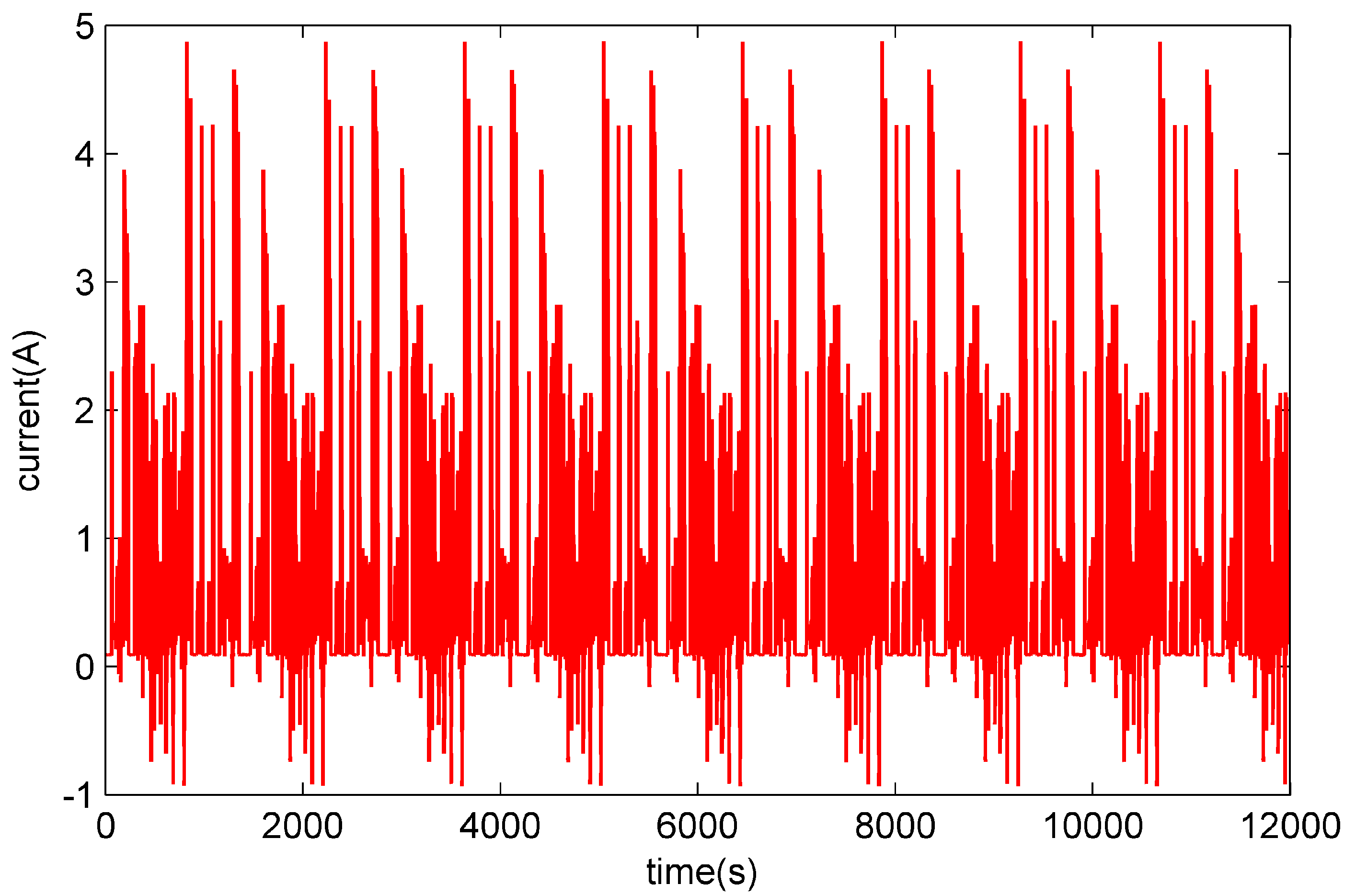
4.1. Battery Test Bench

The structure of the battery test workbench is shown in Figure 3. A Samsung ICR- section P lithium-ion battery (Samsung, Seoul, Korea) was used as the experimental test object. The battery was placed in the battery constant temperature and humidity box (Sanwood, Dongguan, Guangdong, China), and connected with the Arbin battery test equipment (Arbin, College Station, TX, USA). The battery constant temperature and humidity box is used to provide the required battery temperature and humidity conditions, and the PC is connected with the battery test equipment and is used to control the battery test equipment to perform the battery charge and discharge test. The generated data was stored in an SQL database. Matlab R2014a (MathWorks, Natick, MA, USA) was used to analyze the experimental results, and compare the advantages and disadvantages of the algorithms.

4.2. Performance Comparison

In order to compare the performance of the algorithm for the actual work process, the City test was used to simulate the current changes of the battery during the driving of an electric car. A portion of the City operating current is shown in Figure 4. The sampling time is 1 s. The current is positive for discharge, and negative during charging.

4.2.1. Comparison of the Complexity of Methods

The estimation time of the algorithm is greatly influenced by the performance of the hardware, and the estimation time of the algorithm is relatively short if high performance hardware is used. The estimated time of the algorithm is also affected by the details of the program. To control the influence of the above two factors on the algorithm estimation time, three experiments were carried out in the same program running environment, as presented in

Table 1. Time consumption.

Methods	EPF	CPF	UPF
First test	76.655	142.451	161.919
Second test	75.494	139.794	154.117
Third test	67.888	129.757	142.855

. According to the results of the three experiments, we can conclude that the computational cost of the EPF method is much smaller than that of the CPF method and the UPF method, and the computational complexity of the UPF method is slightly larger than that of the CPF method.

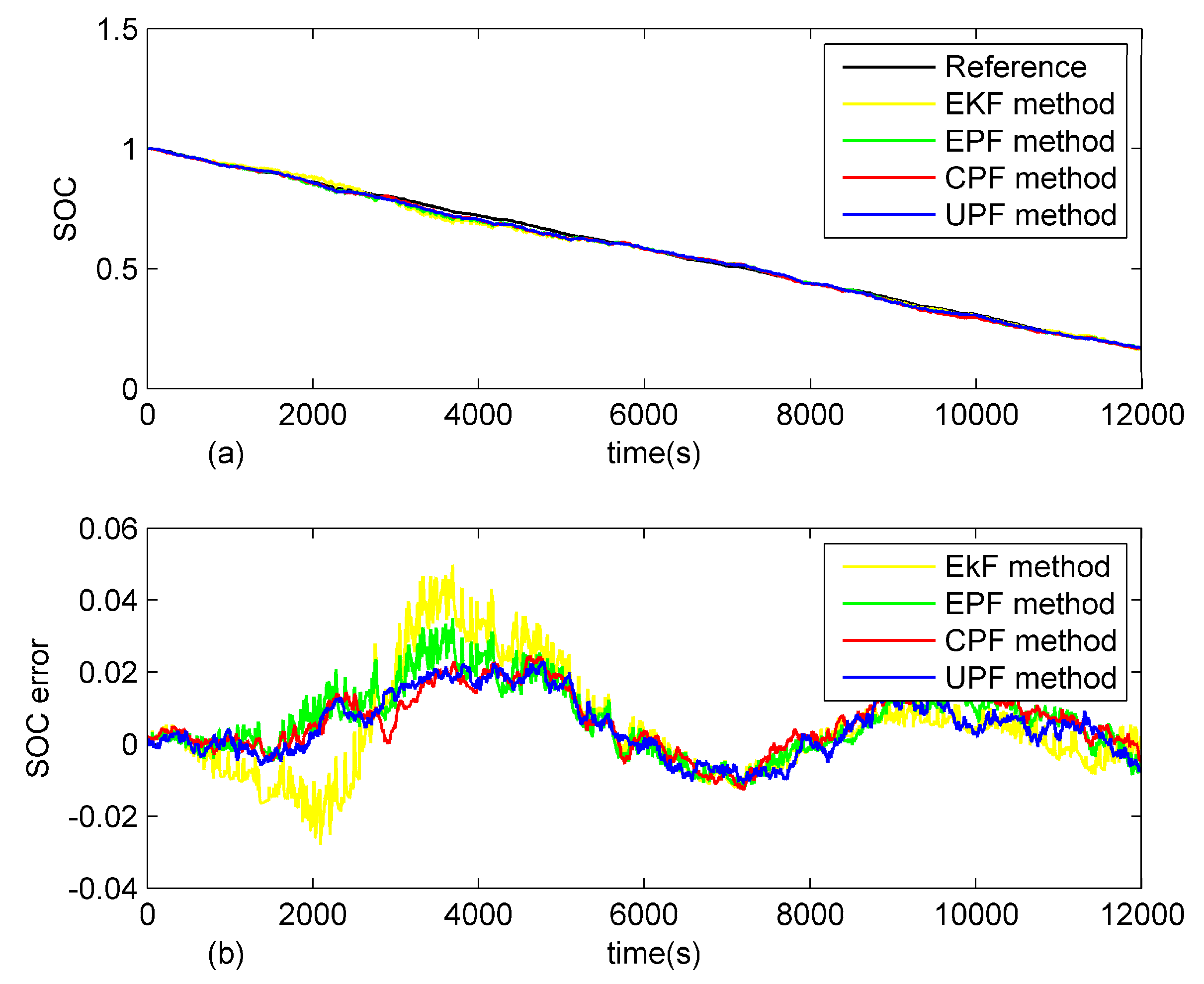
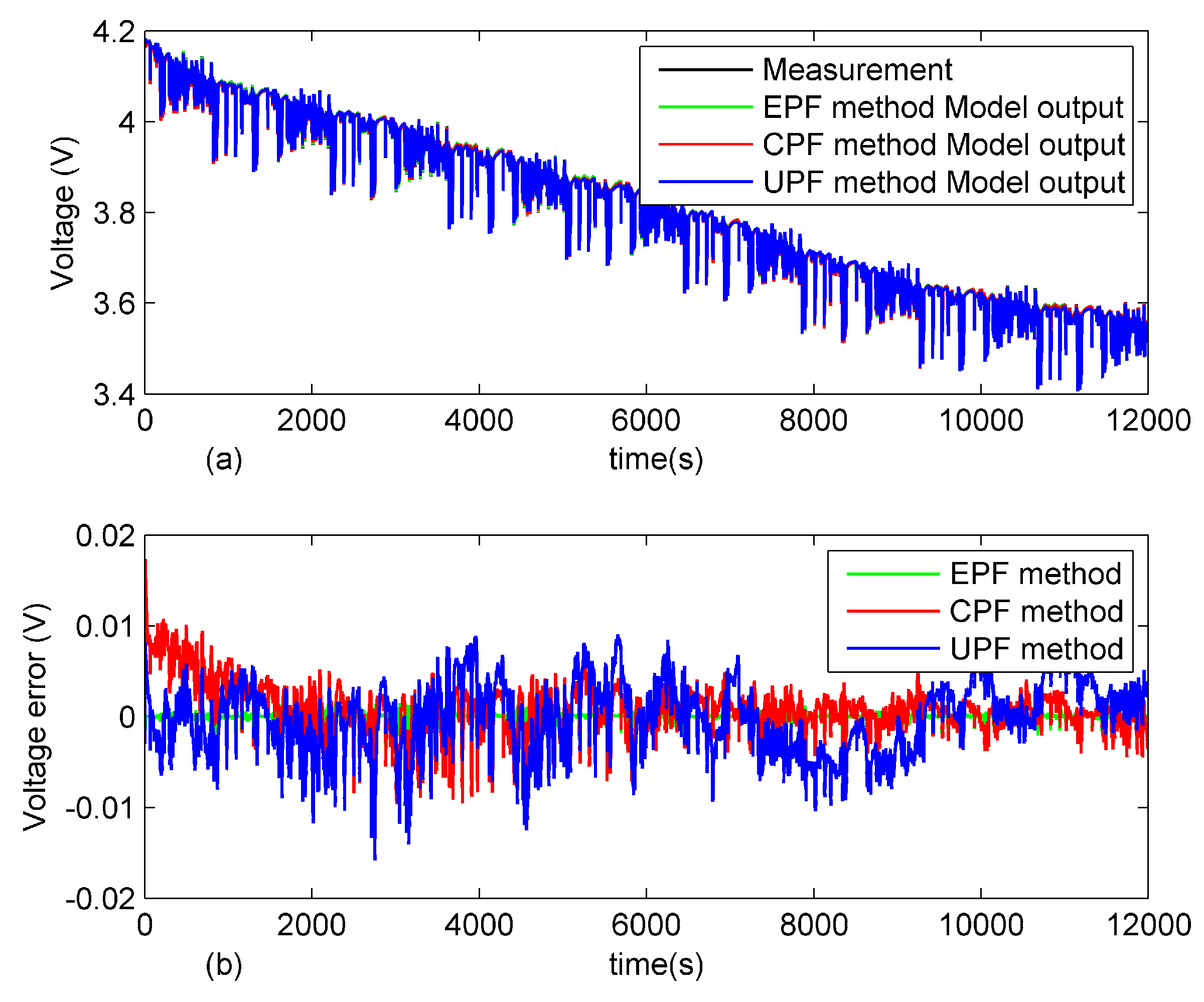
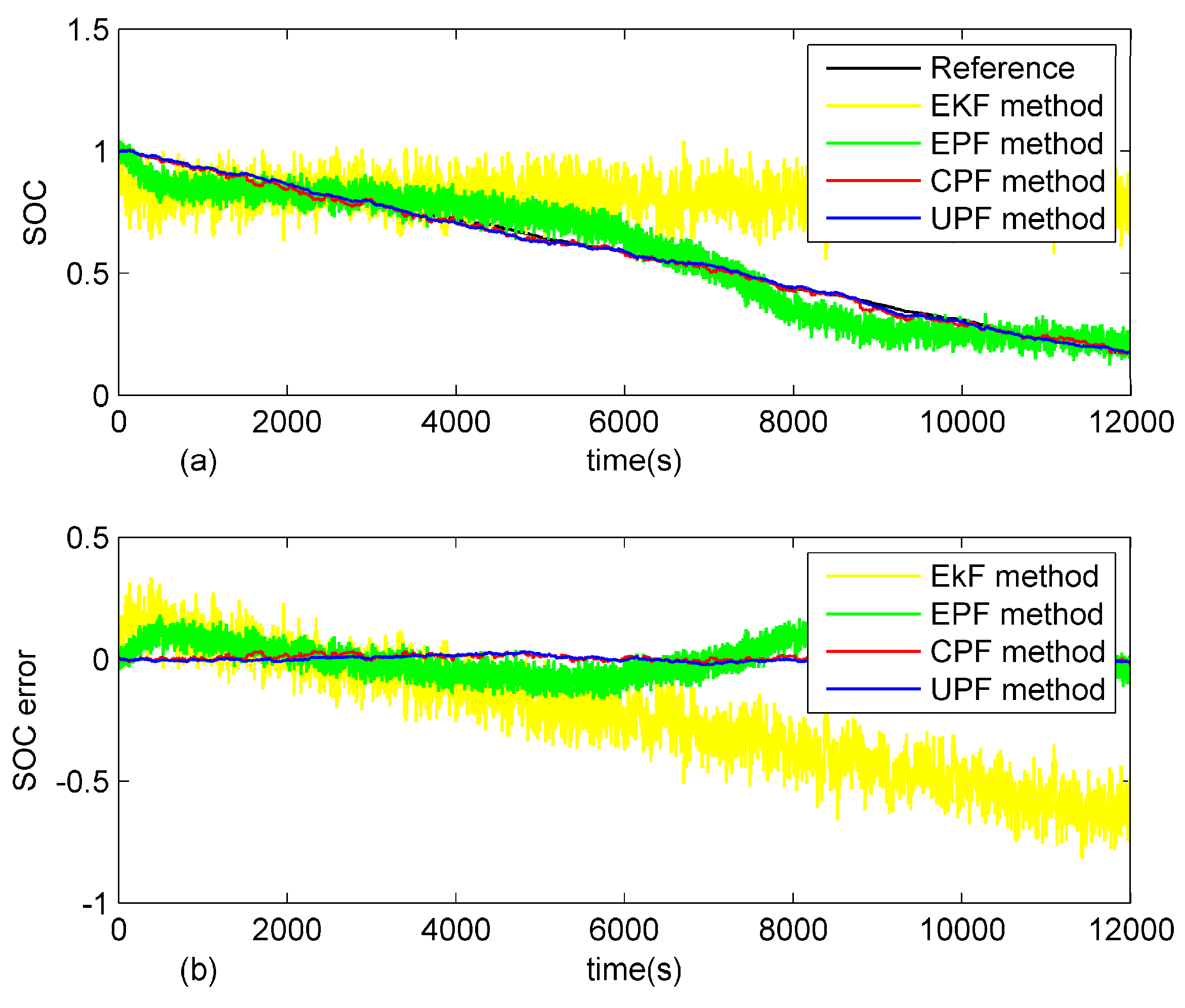
4.2.2. Comparison of the Accuracy and the Model Error of the Methods

The SOC estimation accuracy of the three methods and the estimated battery voltage accuracy were tested under the City test, as shown in Figure 5 and Figure 6. According to the data presented in Figure 5a, the EKF, EPF, CPF, and UPF methods can effectively estimate the SOC value. Figure 5b and

Table 2. Estimated accuracy.

Methods	EKF	EPF	CPF	UPF
Mean absolute error	0.011	0.010	0.009	0.008
Maximum error	0.051	0.034	0.028	0.026

shows the SOC estimation error of the three methods. The SOC estimation error of the EKF method with yellow line and the EPF method represented by the green solid line is larger than that of the other two methods. The SOC estimation error of the UPF method represented by the purple solid line is the smallest, with the best estimation result. Additionally, Figure 6a shows that the three methods can well predict the terminal voltage of the battery using the established second-order RC equivalent circuit model. As shown in Figure 6b, the voltage estimation error of the EPF method is the smallest, and the voltage error of the UPF method is the largest. However, the maximum error is less than 0.02 V for the three algorithms.

4.2.3. Comparison of Robustness

During actual battery operating conditions, the values measured by the current sensor and the voltage sensor tend to contain noise. To maximize actual working conditions, the equations of non-Gaussian noises which have been added into the current and voltage of City test, are respectively:

$$wI=0.2\times \left(r_1-0.5\right)+0.3\times r_2\times wI,wV=0.2\times \left(r_3-0.5\right)+0.3\times r_4\times wV$$

(47)

where $r_1$, $r_2$, $r_3$, $r_4$ represents uncorrelated random numbers between 0 and 1. Figure 7 shows estimation results of the four methods.

Table 3. Performance comparison of four methods in noise environment.

Methods	EKF	EPF	CPF	UPF
Mean absolute error	0.279	0.060	0.011	0.009
Maximum error	0.813	0.199	0.041	0.029

shows the average absolute error and the maximum absolute error in the estimation process of the data shown in Figure 7. According to Figure 7, the EKF method has been ineffective under the condition of adding non-Gaussian noise, and because the PF method has no resistance to non-Gaussian noise, the other three algorithms are better than EKF method. Since the EPF method approximates the nonlinear function of the system by first order linearity, a large error is introduced, which results in the accuracy of the EPF method are lower than those of the CPF method and the UPF method.

5. Conclusions

In this paper, the SOC of a lithium-ion battery was estimated based on EKF, EPF, CPF, and UPF models. The state-space equations were established based on the second-order equivalent circuit model, which is widely used as the lithium-ion battery model. The individual methods were used to identify the parameters in the state-space equations. Compared with the EKF method, EPF, CPF, and UPF methods have great advantages in SOC estimation, especially in the case of a poor environment. The complexity, accuracy, and robustness of the EPF, CPF, and UPF methods were then compared experimentally with the test of the City driving cycle. According to the experimental results, The EPF method is less dependent on hardware than the CPF and UPF methods, therefore, the EPF method should be used if the hardware is insufficient. Although the reliability of the three algorithms is similar with or without noise, the SOC estimation accuracy of the EPF method was lower than that of the CPF method and the UPF method. Therefore, the CPF method and the UPF method should be applied if the hardware condition can be satisfied.

References

1. Yang, N.; Zhang, X.; Li, G. State of charge estimation for pulse discharge of a LiFePO4 battery by a revised Ah counting. Electrochim. Acta 2015, 151, 63–71. [Google Scholar] [CrossRef]
2. Ng, K.S.; Moo, C.-S.; Chen, Y.-P.; Hsieh, Y.-C. Enhanced coulomb counting method for estimating state-of-charge and state-of-health of lithium-ion batteries. Appl. Energy 2009, 86, 1506–1511. [Google Scholar] [CrossRef]
3. Aylor, J.H.; Thieme, A.; Johnson, B.W. A battery state-of-charge indicator for electric wheelchairs. IEEE Trans. Ind. Electron. 1992, 39, 398–409. [Google Scholar] [CrossRef]
4. Lee, S.; Kim, J.; Lee, J.; Cho, B.H. State-of-charge and capacity estimation of lithium-ion battery using a new open-circuit voltage versus state-of-charge. J. Power Sources 2008, 185, 1367–1373. [Google Scholar] [CrossRef]
5. Barbarisi, O.; Vasca, F.; Glielmo, L. State of charge Kalman filter estimator for automotive batteries. Control Eng. Pract. 2006, 14, 267–275. [Google Scholar] [CrossRef]
6. Kim, J.; Cho, B.H. Screening process-based modeling of the multi-cell battery string in series and parallel connections for high accuracy state-of-charge estimation. Energy 2013, 57, 581–599. [Google Scholar] [CrossRef]
7. Vasebi, A.; Bathaee, S.M.T.; Partovibakhsh, M. Predicting state of charge of lead-acid batteries for hybrid electric vehicles by extended Kalman filter. Energy Convers. Manag. 2008, 49, 75–82. [Google Scholar] [CrossRef]
8. Xia, B.Z.; Wang, H.Q.; Tian, Y.; Wang, M.W.; Sun, W.; Xu, Z.H. State of Charge Estimation of Lithium-Ion Batteries Using an Adaptive Cubature Kalman Filter. Energies 2015, 8, 5916–5936. [Google Scholar] [CrossRef]
9. Xia, B.Z.; Wang, H.Q.; Wang, M.W.; Sun, W.; Xu, Z.H.; Lai, Y.Z. A New Method for State of Charge Estimation of Lithium-Ion Battery Based on Strong Tracking Cubature Kalman Filter. Energies 2015, 8, 13458–13472. [Google Scholar] [CrossRef]
10. Sun, T.; Xin, M. Hypersonic entry vehicle state estimation using nonlinearity-based adaptive cubature Kalman filters. Acta Astronaut. 2017, 134, 221–230. [Google Scholar] [CrossRef]
11. Zhigang, H.; Dong, C.; Chaofeng, P.; Long, C.; Shaohua, W. State of charge estimation of power Li-ion batteries using a hybrid estimation algorithm based on UKF. Electrochim. Acta 2016, 211, 101–109. [Google Scholar] [CrossRef]
12. Sun, F.; Hu, X.; Zou, Y.; Li, S. Adaptive unscented Kalman filtering for state of charge estimation of a lithium-ion battery for electric vehicles. Energy 2011, 36, 3531–3540. [Google Scholar] [CrossRef]
13. Pathuri Bhuvana, V.; Unterrieder, C.; Huemer, M. Battery Internal State Estimation: A Comparative Study of Non-Linear State Estimation Algorithms. In Proceedings of the 2013 IEEE Vehicle Power and Propulsion Conference (VPPC), Beijing, China, 15–18 October 2013; pp. 1–6. [Google Scholar]
14. Ye, M.; Guo, H.; Cao, B. A model-based adaptive state of charge estimator for a lithium-ion battery using an improved adaptive particle filter. Appl. Energy 2017, 190, 740–748. [Google Scholar] [CrossRef]
15. Li, J.; Barillas, J.K.; Guenther, C.; Danzer, M.A. A comparative study of state of charge estimation algorithms for LiFePO4 batteries used in electric vehicles. J. Power Sources 2013, 230, 244–250. [Google Scholar] [CrossRef]
16. Aslan, S. Comparison of the hemodynamic filtering methods and particle filter with extended Kalman filter approximated proposal function as an efficient hemodynamic state estimation method. Biomed. Signal Process. Control 2016, 25, 99–107. [Google Scholar] [CrossRef]
17. Yang, Z.; Gui, J.; Shag, S.; Zhao, X.; Zheng, C. EKPF-Based Dynamic State Estimation of Electromechanical Transient Process. Electr. Power 2015, 48, 94–98. [Google Scholar]
18. Sheng-Yun, H.; Hsien-Sen, H.; Tsai-Sheng, K. Extended Kalman Particle Filter Angle Tracking (EKPF-AT) Algorithm for Tracking Multiple Targets. In Proceedings of the 2010 International Conference on System Science and Engineering, Taipei, Taiwan, 1–3 July 2010; pp. 216–220. [Google Scholar]
19. Xia, B.; Sun, Z.; Zhang, R.; Lao, Z. A Cubature Particle Filter Algorithm to Estimate the State of the Charge of Lithium-Ion Batteries Based on a Second-Order Equivalent Circuit Model. Energies 2017, 10, 457. [Google Scholar] [CrossRef]
20. Guo, R.; Gan, Q.; Zhang, J.; Guo, K.; Dong, J. Huber cubature particle filter and online state estimation. Proc. Inst. Mech. Eng. Part I J. Syst. Control Eng. 2017, 231, 158–167. [Google Scholar] [CrossRef]
21. Shen, Y.Q. Hybrid unscented particle filter based state-of-charge determination for lead-acid batteries. Energy 2014, 74, 795–803. [Google Scholar] [CrossRef]
22. He, Y.; Liu, X.; Zhang, C.; Chen, Z. A new model for State-of-Charge (SOC) estimation for high-power Li-ion batteries. Appl. Energy 2013, 101, 808–814. [Google Scholar] [CrossRef]
23. Li, Z.; Huang, J.; Liaw, B.Y.; Zhang, J. On state-of-charge determination for lithium-ion batteries. J. Power Sources 2017, 348, 281–301. [Google Scholar] [CrossRef]
24. Sepasi, S.; Ghorbani, R.; Liaw, B.Y. Inline state of health estimation of lithium-ion batteries using state of charge calculation. J. Power Sources 2015, 299, 246–254. [Google Scholar] [CrossRef]
25. Andre, D.; Meiler, M.; Steiner, K.; Walz, H.; Soczka-Guth, T.; Sauer, D.U. Characterization of high-power lithium-ion batteries by electrochemical impedance spectroscopy. II: Modelling. J. Power Sources 2011, 196, 5349–5356. [Google Scholar] [CrossRef]
26. Zou, C.; Manzie, C.; Nešić, D.; Kallapur, A.G. Multi-time-scale observer design for state-of-charge and state-of-health of a lithium-ion battery. J. Power Sources 2016, 335, 121–130. [Google Scholar] [CrossRef]
27. Xiong, B.; Zhao, J.; Wei, Z.; Skyllas-Kazacos, M. Extended Kalman filter method for state of charge estimation of vanadium redox flow battery using thermal-dependent electrical model. J. Power Sources 2014, 262, 50–61. [Google Scholar] [CrossRef]
28. Tian, Y.; Li, D.; Tian, J.D.; Xia, B.Z. A Comparative Study of State-of-Charge Estimation Algorithms for Lithium-ion Batteries in Wireless Charging Electric Vehicles. In Proceedings of the 2016 IEEE PELS Workshop on Emerging Technologies: Wireless Power Transfer (WoW), Knoxville, TN, USA, 4–6 October 2016; pp. 186–190. [Google Scholar]
29. Doucet, A.; Godsill, S.; Andrieu, C. On sequential Monte Carlo sampling methods for Bayesian filtering. Stat. Comput. 2000, 10, 197–208. [Google Scholar] [CrossRef]
Figure 1. Second-order RC equivalent circuit model.
Energies 10 01149 g001
Figure 2. Experimental results.
Energies 10 01149 g002
Figure 3. The structure of the battery test workbench.
Energies 10 01149 g003
Figure 4. The current profile under the City test.
Energies 10 01149 g004
Figure 5. Comparison of SOC estimation accuracy under the City test: (a) SOC estimation; and (b) SOC estimation error.
Energies 10 01149 g005
Figure 6. Battery model outputs under City test: (a) model output; and (b) model error.
Energies 10 01149 g006
Figure 7. Comparison of estimation results of the four methods in a noisy environment: (a) SOC estimation; and (b) SOC estimation error.
Energies 10 01149 g007