Design of a Control System for a Maglev Planar Motor Based on Two-Dimension Linear Interpolation


School of Electrical Engineering and Automation, Harbin Institute of Technology, Harbin 150001, China
*
Author to whom correspondence should be addressed.
Energies 2017, 10(8), 1132; https://doi.org/10.3390/en10081132
Submission received: 6 June 2017
/
Revised: 23 July 2017
/
Accepted: 27 July 2017
/
Published: 2 August 2017
(This article belongs to the Section I: Energy Fundamentals and Conversion)
Abstract
:In order to realize the high speed and high-precision control of a maglev planar motor, a high-precision electromagnetic model is needed in the first place, which can also contribute to meeting the real-time running requirements. Traditionally, the electromagnetic model is based on analytical calculations. However, this neglects the model simplification and the manufacturing errors, which may bring certain errors to the model. Aiming to handle this inaccuracy, this paper proposes a novel design method for a maglev planar motor control system based on two-dimensional linear interpolation. First, the magnetic field is divided into several regions according to the symmetry of the Halbach magnetic array, and the uniform grid method is adopted to partition one of these regions. Second, targeting this region, it is possible to sample the electromagnetic forces and torques on each node of the grid and obtain the complete electromagnetic model in this region through the two-dimensional linear interpolation method. Third, the whole electromagnetic model of the maglev planar motor can be derived according to the symmetry of the magnetic field. Finally, the decoupling method and controller are designed according to this electromagnetic model, and thereafter, the control model can be established. The designed control system is demonstrated through simulations and experiments to feature better accuracy and meet the requirements of real-time control.
1. Introduction
Planar motion is required for various applications in the high-precision industry, such as pick and place machines, semiconductor lithography, and transport devices [1,2]. Planar movement can be realized through super-accurate 2-D positioning stages. Traditionally, these stages are often constructed by stacking several one-degree-of-freedom linear drives supported by mechanical bearings [3]. However, this type of positioning stage has a high moving mass and low stiffness, which restricts its dynamic performance. In recent years, the 2-D positioning stage has been driven directly by the maglev planar motor [4,5,6,7], which makes it an integrated structure featuring many advantages, such as direct driving, fast response, high sensitivity, good dynamic nature and simple structure [8,9].
A maglev planar motor is a multi-input and multi-output, non-linear and strongly coupled system. The inputs of a maglev planar motor are the currents imposed on each winding, and the outputs are the moving forces on the six degrees of freedom. Solving the corresponding current according to the required forces on the different degrees of freedom is a critical step for achieving six degrees movement of this motor. To realize the position control on the six degrees of freedom of this motor, decoupling the currents of multiple sets of windings and the forces and torques on six degrees of freedom is essential. To obtain this decoupling relation, an accurate electromagnetic model of a maglev planar motor is needed. Meanwhile, this electromagnetic model is supposed to have fast running speed to meet the requirements of high dynamic response of the control system. Therefore, on the basis of meeting the requirements of real-time running speed, a more precise electromagnetic model is indispensable for a high speed and high precision maglev planar motor control system.
It has been concluded in [10] that the surface charge model and harmonic model have high model accuracy, but they are not suitable for practical implementation because the computation time needed is too long, often within the scale of seconds. On the other hand, analytical models have relatively lower model accuracy (still deemed high enough for industrial applications) but the computation time needed (normally less than 2 μs) on a typical DSP control system is very small. Therefore, the analytical method has been widely used in the planar motor control implementation.
Hamers points out three analytical ways to solve magnetic force in his research report, namely the virtual work method, Maxwell stress method, and the Lorentz force equation method [11]. Normally, the Lorentz force equation method can compute the electromagnetic force and torque of the coils in a maglev planar motor, which is the most convenient method and widely adopted in establishing electromagnetic models of the maglev planar motor [12,13,14]. However, this method can not be directly used to calculate the electromagnetic force on the corner segment of the coil, therefore, the shape of the real coil needs to be simplified. In [15], the coils are simplified into four rectangles, but there are overlapping parts during the calculation process. In [16], the winding is regarded as four trapezoids, which reduces the overlapping parts. However, this simplified model still takes a right angle as a real circle corner. Reference [17] proposes a method that converts the electromagnetic force and torque modeling of the corner coils to the polar coordination system. This method can improve the accuracy of the electromagnetic force and torque of the corner coils. However, in all the methods above, in order to achieve the real-time computation, the Lorentz force equation method only takes the fundamental component of magnetic flux density into account. As a result, the ignored harmonic components will cause relatively significant errors in the electromagnetic model.
An improved semi-analytical method based on a single-point magnetostatic field simulation is proposed in [18] to get a more accurate electromagnetic model. This method does not assume the relative permeability to be 1 as done in many traditional models. Moreover, it does not neglect the difference between the attractive force and the repulsive force. However, the needed computation time is too long to make it suitable for real-time implications. In [19], numerical calculations and a measurement setup are used to model the force and torque generated by each coil. A novel single-deck six degree of freedom magnetic levitation stage has been introduced in [20] which also analyzes semi-empirical equations of the motor and furthermore builds a model based on the ratio of the measured force to the current. The forces in the direction of x/y/z are generated by different coil arrays, thus only one-dimensional fitting has been adopted due to the lack of electromagnetic coupling.
Interpolation is a mathematical method to get a continuous function based on discrete data points, and makes all the original data points located on the new continuous curve. The interpolation is an important method for the approximation of discrete functions, and it can estimate the approximate value of other points based on the original data points. Interpolation can get the complete model based on limited measured data points; moreover, the dimensions can be easily extended if needed. Therefore, it has been widely used in numerous application fields [21,22,23,24].
In order to minimize the errors arising from the model simplification and manufacturing process and to meet the requirements of real-time control simultaneously, this paper proposes a new method to obtain accurate electromagnetic force and torque based on the two-dimensional interpolation method. Based on the above method, the decoupling computation of the maglev planar motor can be realized and a high performance real-time control model can be designed.
2. Analysis Model of Maglev Planar Motor
2.1. Structure and Working Principle
Figure 1 shows the moving-coil ironless maglev permanent magnet planar motor. It consists of a mover, a stator, and the gap between them. The mover consists of the base plate and the 4×4 coil array, and the stator consists of the yoke plate and the permanent magnet array. The stator permanent magnet is arranged in a Halbach structure, which can increase the flux density near the coils. The coils on the mover are connected to the outer power supply. More specifically, each coil is supplied by one independent current amplifier, thus the decoupled current can be realized through the connected independent power supply.
The working principle of the proposed planar motor is described as follows. The permanent magnet generates a magnetic field, in which the coils with current in them will generate electromagnetic force and electromagnetic torque. Since the magnets array remains still, the electromagnetic force and torque on the whole coils drive the mover move. As long as the proper current according to the relative position between the coils and the magnetic field are given, the control of electromagnetic force and torque on six degrees of freedom can be realized and the position control of the mover on six degrees of freedom can be achieved.
2.2. Coordinate Definition and Transformation
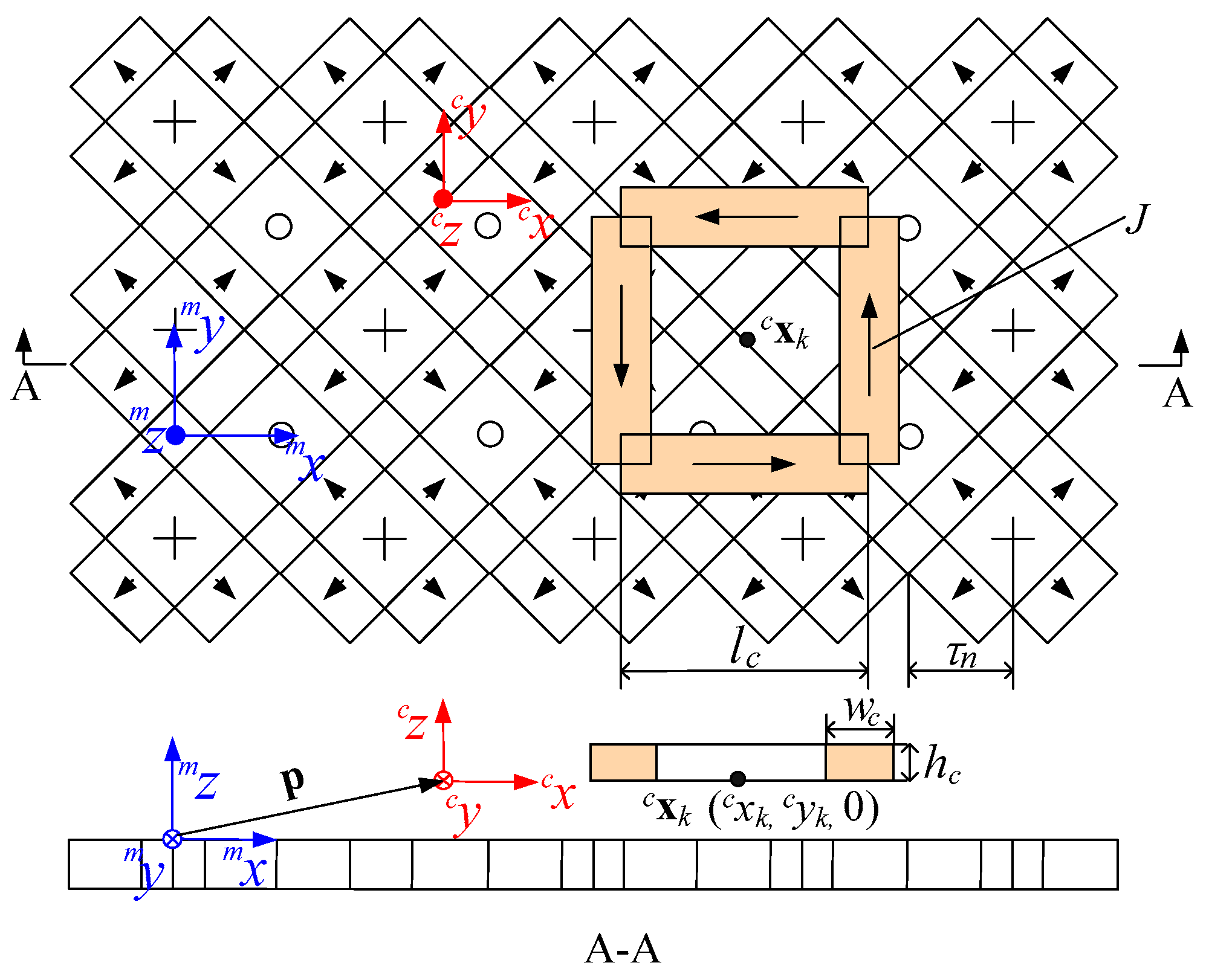
In Figure 2, the coil is divided into four straight segments. τn denotes the pole pitch, lc denotes the coil length of the straight coil segment, hc is the thickness of the coil, wc is the width of the coil, J is current density. Two different coordinate systems are defined in Figure 2.
The first one is the stator global coordinate system denoted with the superscript m, which is fixed on the top face of the stator permanent magnet. It can be expressed as:
The second one is the mover local coordinate system denoted with the superscript c, which is fixed on the mover bottom surface center. It can be expressed as:
The coordinate position of the k-th coil center in the mover local coordinate system can be expressed as:
The position vector transformation between the mover local coordinate system and the stator global coordinate system is expressed as:
The vector in the mover local coordinate system and that in the stator global coordinate system can be transformed into each other through the following [25,26]:
The orientation transformation matrix is defined as:
where, ϕ, θ and φ are the rotation angles about the cx-, cy-, and cz-axes, respectively.
2.3. Electromagnetic Force and Torque
According to the Lorenz’s law, the electromagnetic force and torque on the coil can be derived as:
where, B is the flux density distribution of the magnet array; J is the current density in the coil; V is the volume of the coil; r is the vector from the point about which the torque is calculated.
In the mover local coordinate system, the electromagnetic force and torque on the straight segment of the coil can be derived as:
where, cBxy is the flux density distribution component on x-y plane. Cz can be expressed as:
Based on Equations (14) and (15), the electromagnetic force and torque on the k-th coil can be derived as:
where, C1 and C2 are the coefficients related to the motor structure; C is harmonic compensation factor; crz is the equivalent force arm in the cz-direction from the coil to the mover mass center.
Once the coil is put on the mover, the position deviation on the x-y plane can be seen as constant, therefore, the whole electromagnetic force and torque on the mover is the sum result of that on each winding, taking the position deviation into account.
3. Design of the Control System
3.1. Electromagnetic Model Based on Two-Dimensional Linear Interpolation
Analytical modeling seeks mathematical functions and equations that are obtained from the closed-form (exact or approximate) solution to the original physics-governing equations. The outcome of analytical modeling is behavioral models [27]. For instance, Equations (17)–(22) provide the analytical modeling for the electromagnetic force/torque of the maglev planar motor. The interpolation method, on the other hand, processes the discrete data with the numerical approach based on the known data, thus a complete mathematical model of the control target object can be derived. Normally, interpolation includes linear interpolation, polynomial interpolation, cubic spline interpolation, which extend from single dimension to multiple dimensions [28]. To meet the real-time computation needs, both the accuracy and speed should be taken into account to choose a proper interpolation method; therefore, the two-dimension interpolation method has been chosen.
3.1.1. Interpolation Region Partition
Since the magnetic field of a Halbach array is strictly periodic symmetrical, it can be simplified to take points in a small range to perform the interpolation. The whole planar model can be derived from this symmetric characteristic. After taking these sampling points, the precious relation between position, current, electromagnetic force and torque can be obtained from two-dimension interpolation method, thus a precious real-time control model can established.
The interval 0–2τn is partitioned into four regions according to the symmetry of the magnetic field, as shown in Figure 3. Thus, the corresponding relation between the current and electromagnetic force and torque in other regions can be deducted from the interpolation results in region I as shown in Figure 3.
3.1.2. Interpolation Calculation
Bilinear interpolation method is adopted to interpolate in region I of Figure 3 with. After the partition in region I, the interpolation points (xg, yh) are located within:
Then the value of interpolation point s(xg, yh) can be determined by the value on (xi, yj), (xi+1, yj), (xi, yj+1), (xi+1, yj+1).
The value on the interpolation point can be calculated:
where:
When interpolating with Equation (27), the feedback position of maglev planar motor’s mover under global coordination system is s(xg, yh), thus, the corresponding electromagnetic model can be obtained.
3.2. Current Decoupling
The input of the maglev planar motor is the current in each coil and the output is the force and torque on the mover. It is a multi-input and multi-output coupling system. Thus, the decoupling current control of each coil is extra critical to realize the overall performance of the control system. In the proposed maglev planar motor, there are 16 sets of independent coils. Each coil can generate the forces and torques in multiple degrees of freedom. The total force and torque on the mover mass center can be seen as the sum of those on the 16 coils. The force and torque on the mover can be expressed as:
The current in each coil of the mover and the electromagnetic force and torque of the mover can be expressed as:
where, p is the position vector; K(p) is a coefficient matrix about the electromagnetic force and torque relevant to the position.
Each element in K(p) is the relation of the corresponding current and force, this relation can be obtained from analytical method or sampling and interpolation. The Moore-Penrose generalized inverse matrix of K(p) is shown as:
The current in each coil can be obtained as:
3.3. Dynamic Model
The coil and the back plate of the moving-coil maglev planar motor are deemed as one object, which forms the mover of this motor, and this can be regarded as rigid motion. Based on the above analysis, the rigid body dynamic of the mover can be described as:
where, m is the mover mass; g is the gravitational acceleration; Ix, Iy and Iz are rotary inertia.
3.4. Control System Structure
After the decoupling of the six degree of freedom maglev permanent magnetic synchronous planar motor, six independent single degree of freedom control system can be derived. Thus, an independent controller applied on each single degree of freedom can achieve the corresponding closed loop control. Thereafter, the multi-degree of freedom control of the six degrees maglev motor can be achieved.
In order to achieve the six dimension control of the maglev planar motor, a closed loop control is needed for each dimension. The current can be calculated according to the required electromagnetic force and torque and the relative position of the magnetic field. In Figure 4, pref is the given position vector; Wref is the needed force and torque on each degree of freedom; iref is the needed current in each coils; W is the generated forces and torques on the six degrees of freedom; and p is the displacement vector of the planar motor.
3.5. Controller Design
A PID controller has the advantages of simple structure and being easy to control, and it can get the desired control results under certain external conditions, therefore, it is widely used in the industrial control field [29,30,31,32,33]. Through the PID controller, the system can process the proportional, integral and differential calculation, and output the sum of the three calculations as the control signal for the controlled object. According to the characteristics of the controlled object and the required performance, the controller can be conducted as P control, PI control and PID control.
3.5.1. Control Law Analysis
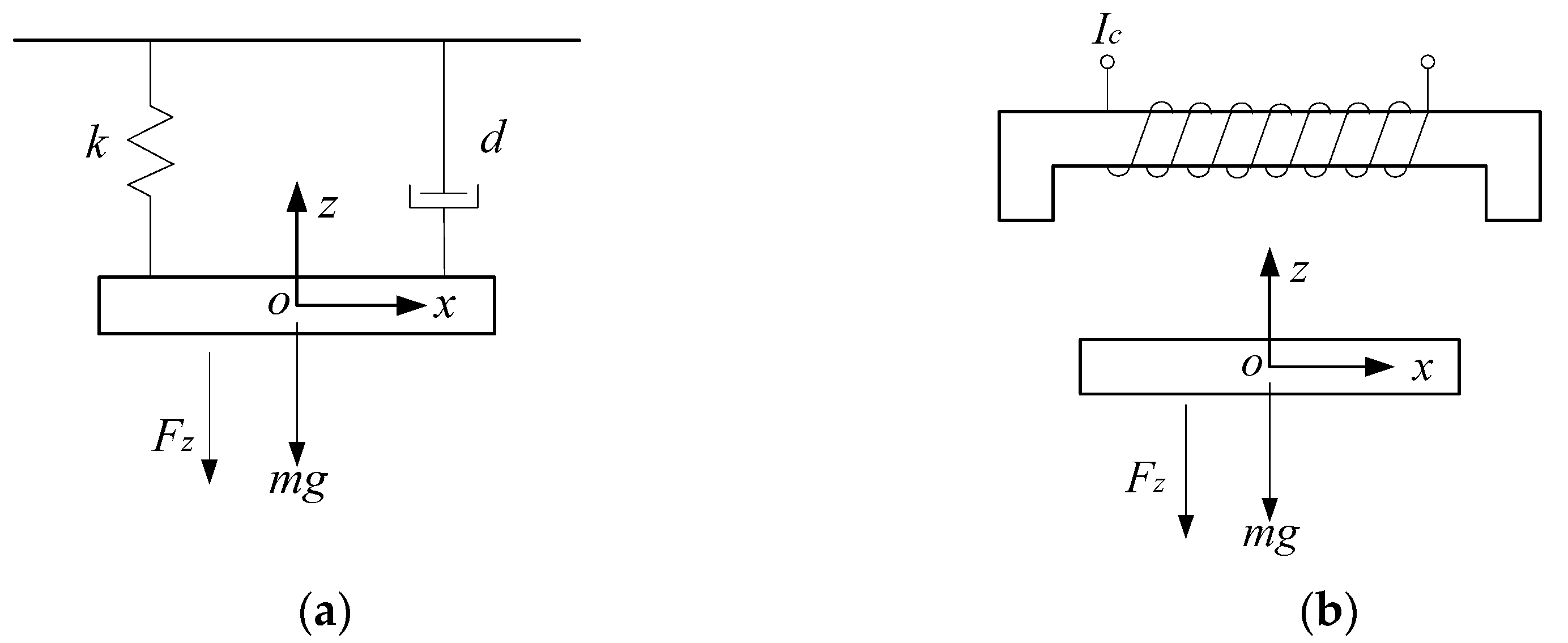
A maglev system is a non-linear and open loop unstable system, the linearized model consists of displacement stiffness coefficient and current stiffness coefficient, but what differs from the general spring damp system is that the displacement stiffness coefficient of this system is negative without feedback control. The controlled object can only be suspended and remain stable with certain disturbance when imposing enough current on the coil. The adjustment and choose of the maglev system can be explained through Figure 5.
In Figure 5b, the kinematics equation of the maglev system is:
Make the two systems equivalent:
Therefore, the control law of the current is chosen as:
where:
Equation (43) demonstrates that in order to make the two systems to be equivilent, the current of the controlled maglev system is supposed to consist of at least a proportional control part and differntial control part. From the perspective of mechanical engineering, the proportional part of the current is used to offset the restoring force caused by the negative stiffness and change the system into positive stiffness. The differential part of the current is used to make the system of positive damping, and thus of sufficient stability.
3.5.2. Controller Struture
From the analysis of the previous section, in order to realize the stable suspension of the controlled object, there must be proportional and differential law in this closed loop controller. Meanwhile, to neglect and minimize the stable error of this system, integral control law can be added into this control system.
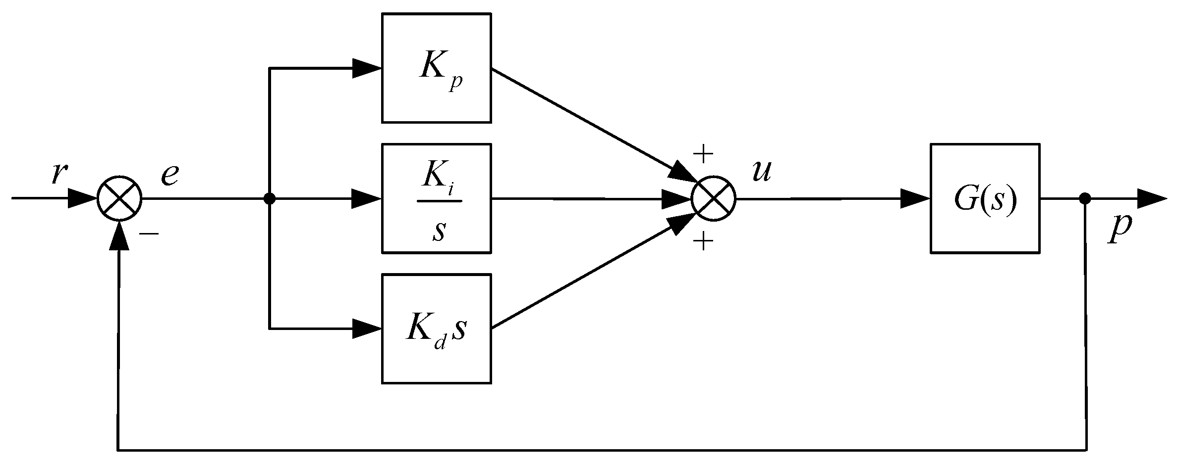
The time domain expression of this PID controller is:
The general transfer function of the PID controller is:
where, Kp is the proportional gain; Ki is the integral gain; Kd is the differential gain.
The structure of this PID controller is shown in Figure 6, where r is the system reference value, u is the control value, G(s) is the controlled object, p is the system output. The proportional component provides the overall control of the different error e, the integral component minimizes the stable error through low frequency integral compensation, and differential component improves the dynamic response through high frequency differential compensation.
4. Validation and Analysis
The validation and analysis consists of three parts. First, the precision of the model is analyzed through 3-D finite element method (FEM) simulation. Then the precision of the control system is analyzed through MATLAB/Simulink simulation. Finally, the real time ability of this system has been validated and analyzed. The parameters of the planar motor for the validation and analysis are shown in Table 1.
4.1. Model Accuracy Analysis
The 3-D simulation is applied to validate the accuracy of the analytical model and the interpolation model respectively.
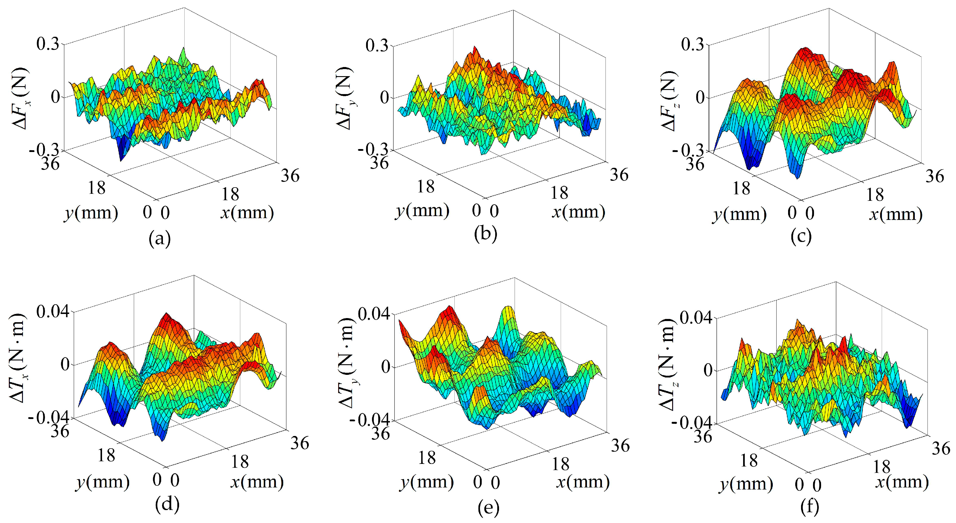
In Figure 7 and Figure 8, the displacement in the direction of x is from 0 mm to 36 mm, the same displacement length and the same sampling method are applied to the direction of y. The parameters for the simulation are shown in Table 1, and a current of 3 A is imposed on the coil. The amplitude of Fx, Fy, Fz, Tx, Ty, and Tz calculated by FEM are 12.39 N, 12.39 N, 25.67 N, 1.68 N·m, 1.69 N·m, and 1.83 N·m, respectively. It can be seen from Figure 7 that the maximum absolute value errors are 0.83 N for Fx, 0.91 N for Fy, 2.38 N for Fz, 0.154 N·m for Tx, 0.166 N·m for Ty, and 0.148 N·m for Tz. Figure 8 shows the error between the interpolation model and 3-D simulation. It can be seen from Figure 8 that the maximum absolute value errors are 0.18 N for Fx, 0.16 N for Fy, 0.23 N for Fz, 0.033 N·m for Tx, 0.038 N·m for Ty, and 0.032 N·m for Tz. It has been found from the comparison above that interpolation method has a better model accuracy than the analytical method.
After the decoupling, the originally strongly decoupled system becomes a weakly decoupled system. However, the decoupling performance depends on the modeling accuracy. The model decoupling and its control parts together determine the position loop accuracy of the whole control system. Under a given position loop accuracy, a high modeling accuracy can make the other parts in the control system, like the decoupling and noise filtering, relatively easier and thus more efficient. Therefore, it is easier to realize the desired position loop accuracy goal.
4.2. System Precision Analysis
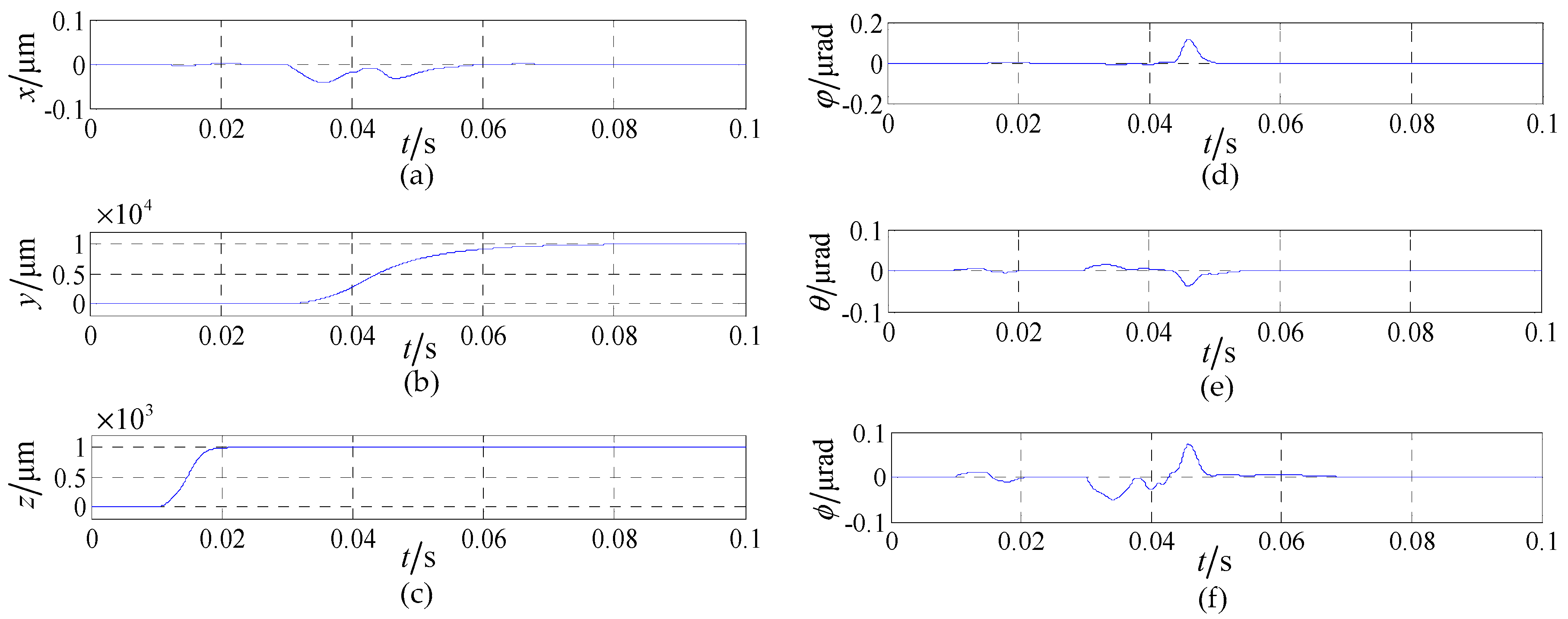
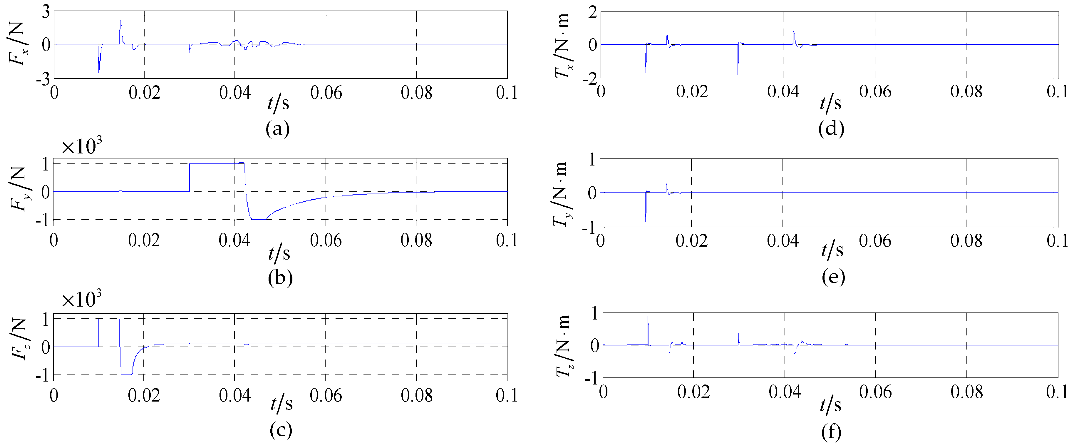
Through MATLAB/Simulink software, the control system is established as shown in Figure 4, and it consists of six PID controllers to realize the control on the six degrees of freedom. The parameters of motor are as shown in Table 1. The simulation time is set as 0.1 s, and 1 mm displacement reference order on z-direction is given at 0.01 s, which is the working suspension height of the maglev planar mover. 10 mm position step signal on y-direction is given at 0.03 s, and the reference order remains to be 0 on the rest directions to observe the decoupling performance. Upon the simulation above, the displacement curve and the force/toque curve from the control system based on the traditional analytical method is shown in Figure 9 and Figure 11. The displacement curve and the force/torque curve from the control system based on the two-dimension linear interpolation method are shown in Figure 10 and Figure 12.
In Figure 9, the position disturbance on x-axis caused by y-axis and z-axis position variation is from −0.081 μm to 0.076 μm, the position disturbance on ϕ-axis is from −0.51 μrad to 0.73 μrad, the position disturbance on θ-axis is from −0.23 μrad to 0.21 μrad, the position disturbance on φ-axis is from −0.38 μrad to 0.35 μrad. In Figure 10, because of the position variation of y-axis and z-axis, the position disturbance of x-axis is from −0.038 μm to 0.004 μm, the position disturbance of ϕ-axis is from −0.003 μrad to 0.12 μrad, the position disturbance of θ-axis is from -0.035 μrad to 0.013 μrad, the position disturbance of φ-axis is from −0.058 μrad to 0.078 μrad.
Figure 11 shows the force and torque disturbance caused by y-axis and z-axis position variation: for Fx, it varies from −2.65 N to 2.48 N; For Tx, it varies from −1.86 N·m to 0.79 N·m; For Ty, it varies from −0.91 N·m to 0.16 N·m; For Tz, it varies from −0.27 N·m to 0.95 N·m. Due to the saturation restriction of the controller, the forces on y-axis and z-axis are limited within ±1000 N. In Figure 12, it shows the force and torque disturbance caused by y-axis and z-axis position variation: for Fx, it varies from −0.57 N to 0.13 N; For Tx, it varies from −0.13 N·m to 0.07 N·m; For Ty, it varies from −0.005 N·m to 0.086 N·m; For Tz, it varies from −0.089 N·m to 0.052 N·m.
Figure 13 shows the difference of the forces and torques in FEM, analytical method and interpolation method. It has been found that the interpolation method is more close to the FEM than the analytical method. Through the comparison of the simulation results, it can be seen that the control system based on the interpolation method takes into account not only the model simplification, but also the error of materials manufacturing, processing and installation, which makes the established electromagnetic model reflect the real physical model better. Therefore, the established model is of higher position precision.
4.3. Model Real-Time Verification
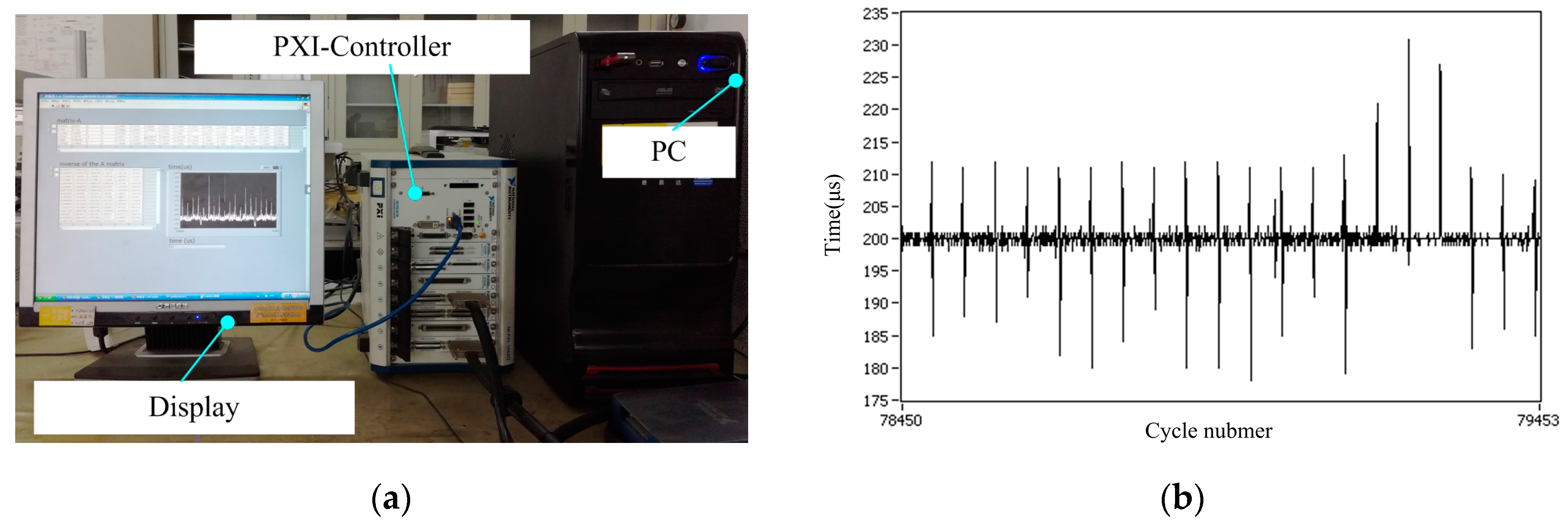
We programmed the proposed interpolation model and ran it on a NI PXI 1042Q real time platform to verify the real time ability. Figure 14a shows the real time control platform, including an industrial PC, embedded controller, plug-in I/O module, a PC and a display. PC connects the real time controller via a cable, and the PC is used to write LabVIEW program and download it to the controller. Controller needs to complete the real time computation of the program, read data from I/O board and upload data to the PC.
Figure 14a shows the measured results of the running time for each loop. From Figure 14b, it can be seen that the average running time of the proposed model based on two-dimensional interpolation is 200 μs and the maximum value is 232 μs.
Table 2 shows the computation time of each modeling method. The model size of FEM is 0.2 m × 0.2 m × 0.1 m, which has been further divided into about 3 mm2 units. The simulation time is about 1 h. Numerous points need to be simulated to get the force on a certain plane. FEM takes a large amount of time and thus it is suitable for theoretical validation. The computation times for the analytical method and interpolation method are quite similar. On the NI control platform it is about 200 μs. For real-time control, it is normally required that the computation time be less than 1 ms. Thus, both of the two above methods are suitable for the real-time control system in industrial applications. However, the interpolation method is more accurate than the analytical method.
5. Conclusions
This paper proposes an electromagnetic model establishing method based on two-dimensional linear interpolation, and designs a maglev planar motor control system accordingly. The proposed model can reduce the model simplification and the manufacturing error, and thus better represents the real physical model. The 3-D FEM simulation approach is used to validate the proposed model error and the analytical model error, respectively. The validation result shows that the proposed model is found to have smaller model error. Adopting MATLAB/Simulink to build the control system, comparing the control system position precision based on the two models, it shows the control system based on the two-dimensional linear interpolation method is of higher position precision. Meanwhile, NI-PXI platform is used to validate the real-time ability of the control model, the average running time is 200 μs. Thus, it can be concluded that the proposed control model is more suitable to be applied in the high speed and high precision maglev planar control system.
Acknowledgments
This work was supported in part by the National Science and Technology Major Project (2009ZX02207-001), in part by the China Postdoctoral Science Foundation Funded Project (2015M80262), in part by the State Key Program of National Natural Science of China under Grant (51537002), in part by the Natural Science Foundation of Heilongjiang Province (E2016035), in part by the National Natural Science Foundation of China (51607044), and in part by “the Fundamental Research Funds for the Central Universities” (Grant No. HIT. NSRIF. 2017010).
Author Contributions
Design of the research scheme and research supervision: Feng Xing, Baoquan Kou, and Lu Zhang. Performing of the research and writing of the manuscript: Xiangrui Yin and Yiheng Zhou.
Conflicts of Interest
The authors declare no conflict of interest.
References
- Rovers, J.M.M.; Jansen, J.W.; Compter, J.C.; Lomonova, E.A. Analysis method of the dynamic force and torque distribution in the magnet array of a commutated magnetically levitated planar actuator. IEEE Trans. Ind. Electron. 2012, 59, 2157–2166. [Google Scholar] [CrossRef]
- Nguyen, V.H.; Kim, W.J. Design and control of a compact lightweight planar position moving over a concentrated-field magnet matrix. IEEE Trans. Mechatron. 2013, 18, 1090–1099. [Google Scholar] [CrossRef]
- Jansen, J.W.; Lomonova, E.A.; Vandenput, A.J.A.; Van Lierop, C.M.M. Analytical model of a magnetically levitated linear actuator. In Proceedings of the Fourtieth IAS Annual Meeting, IEEE Industry Applications Conference, Hong Kong, China, 2–6 October 2005; pp. 2107–2113. [Google Scholar]
- Jansen, J.W.; Smeets, J.P.C.; Overboom, T.T. Overview of analytical models for the design of linear and planar motors. IEEE Trans. Magn. 2014, 50, 39–52. [Google Scholar] [CrossRef]
- Zhang, L.; Kou, B.Q.; Li, L.Y. Modeling and design of an integrated winding synchronous permanent magnet planar motor. IEEE Trans. Plasma Sci. 2013, 41, 1214–1219. [Google Scholar] [CrossRef]
- Ueda, Y.; Ohsaki, H. A Planar actuator with a small mover traveling over large yaw and translational displacements. IEEE Trans. Magn. 2008, 44, 609–616. [Google Scholar] [CrossRef]
- Christian, S.R.J.; Kim, W.J. Multivariable control and optimization of a compact 6-DOF precision positioner with hybrid H2/H∞ and digital filtering. IEEE Trans. Control Syst. Technol. 2013, 21, 1641–1651. [Google Scholar]
- Jansen, J.W.; van Lierop, C.M.M.; Lomonova, E.A. Magnetically levitated planar actuator with moving magnets. IEEE Trans. Ind. Appl. 2008, 44, 1108–1115. [Google Scholar] [CrossRef]
- Zhang, L.; Kou, B.Q.; Zhang, H.; Guo, S.L. Characteristic analysis of a long-stroke synchronous permanent magnet planar motor. IEEE Trans. Magn. 2012, 48, 4658–4661. [Google Scholar] [CrossRef]
- Jansen, J.W. Magnetically Levitated Planar Actuator with Moving Magnets: Electromechanical Analysis and Design. Ph.D. Thesis, Eindhoven University of Technology, Eindhoven, The Netherlands, 2007. [Google Scholar]
- Hamers, H.R. Actuation Principles of Permanent Magnet Synchronous Planar Motors: A Literature Survey; Working Paper; Eindhoven University of Technology: Eindhoven, The Netherlands, 2005. [Google Scholar]
- Van Lierop, C.M.M.; Jansen, J.W.; Damen, A.A.H.; Lomonova, E.A.; van den Bosch, P.P.J.; Vandenput, A.J.A. Model-based commutation of a long-stroke magnetically levitated linear actuator. IEEE Trans. Ind. Appl. 2009, 45, 1982–1990. [Google Scholar] [CrossRef]
- Peng, J.R.; Zhou, Y.F.; Liu, G.D. Calculation of a new real-time control model for the magnetically levitated ironless planar motor. IEEE Trans. Magn. 2013, 49, 1416–1422. [Google Scholar] [CrossRef]
- Xu, F.Q.; Dinavahi, V.; Xu, X.Z. Parallel computation of wrench model for commutated magnetically levitated planar actuator. IEEE Trans. Ind. Electron. 2016, 63, 7621–7631. [Google Scholar] [CrossRef]
- Jansen, J.W.; van Lierop, C.M.M.; Lomonova, E.A.; Vandenput, A.J.A. Modeling of magnetically levitated planar actuators with moving magnets. IEEE Trans. Magn. 2007, 43, 15–25. [Google Scholar] [CrossRef]
- Verma, S.; Shakir, H.; Kim, W.J. Novel electromagnetic actuation scheme for multiaxis nanopositioning. IEEE Trans. Magn. 2006, 42, 2052–2062. [Google Scholar] [CrossRef]
- Zhu, H.Y.; Teo, T.J.; Pang, C.K. Design and modeling of a six degrees-of-freedom magnetically levitated positioner using square coils and 1D halbach arrays. IEEE Trans. Ind. Electron. 2016, 64, 440–450. [Google Scholar] [CrossRef]
- Zhang, H.; Kou, Q.B.; Jin, Y.X.; Zhang, H.L. Modeling and analysis of a new cylindrical magnetic levitation gravity compensator with low stiffness for the 6-DOF fine stage. IEEE Trans. Ind. Electron. 2015, 62, 3629–3639. [Google Scholar] [CrossRef]
- Berkelman, P.; Dzadovsky, M. Magnetic levitation over large translation and rotation ranges in all directions. IEEE/ASME Trans. Mechatron. 2013, 18, 44–52. [Google Scholar] [CrossRef]
- Lai, Y.C.; Lee, Y.L.; Yen, J.Y. Design and servo control of a single-deck planar maglev stage. IEEE Trans. Magn. 2007, 43, 2600–2602. [Google Scholar] [CrossRef]
- Zeng, Z.P.; Triozon, F.; Barraud, S.; Niquet, Y.M. A Simple interpolation model for the carrier mobility in trigate and gate-all-around silicon NWFETs. IEEE Trans. Electron. Devices 2017, 64, 2485–2491. [Google Scholar] [CrossRef]
- Chen, Y.D.; Li, L. Smooth geodesic interpolation for five-axis machine tools. IEEE/ASME Trans. Mechatron. 2016, 21, 1592–1603. [Google Scholar] [CrossRef]
- Tang, J.J.; Ni, F.; Ponci, F.; Monti, A. Dimension-adaptive sparse grid interpolation for uncertainty quantification in modern power systems: Probabilistic power flow. IEEE Trans. Power Syst. 2016, 31, 907–919. [Google Scholar] [CrossRef]
- Huang, X.D.; Jing, S.X.; Wang, Z.H.; Xu, Y.; Zheng, Y.Q. Closed-form FIR filter design based on convolution window spectrum interpolation. IEEE Trans. Signal Process. 2016, 64, 1173–1186. [Google Scholar]
- Craig, J.J. Introduction to Robotics: Mechanics and Control, 3rd ed.; Pearson Prentice Hall: Upper Saddle River, NJ, USA, 2005; pp. 19–48. [Google Scholar]
- Jansen, J.W.; van Essen, J.M.; van Lierop, C.M.M.; Lomonova, E.A.; Vandenput, A.J.A. Design and test of an ironless, three degree-of-freedom, magnetically levitated linear actuator with moving magnets. In Proceedings of the IEEE International Conference on Electric Machines and Drives, San Antonio, TX, USA, 15 May 2005; pp. 858–865. [Google Scholar]
- Li, D.Q. Encyclopedia of Microfluidics and Nanofluidics; Springer Science & Business Media: New York, NY, USA, 2008; p. 47. [Google Scholar]
- Press, W.H. Numerical Recipes: The Art of Scientific Computing, 3rd ed.; Cambridge University Press: Cambridge, UK, 2007; pp. 110–196. [Google Scholar]
- Wang, J.S.; Yang, G.H. Data-driven output-feedback fault-tolerant compensation control for digital PID control systems with unknown dynamics. IEEE Trans. Ind. Electron. 2016, 63, 7029–7039. [Google Scholar] [CrossRef]
- Song, Y.D.; Huang, X.; Wen, C.Y. Robust adaptive fault-tolerant PID control of MIMO nonlinear systems with unknown control direction. IEEE Trans. Ind. Electron. 2017, 64, 4876–4884. [Google Scholar] [CrossRef]
- Pounds, P.E.I.; Dollar, A.M. Stability of helicopters in compliant contact under PD-PID control. IEEE Trans. Robot. 2014, 30, 1472–1486. [Google Scholar] [CrossRef]
- Ang, K.H.; Chong, G.; Li, Y. PID control system analysis, design, and technology. IEEE Trans. Control Syst. Technol. 2005, 13, 559–576. [Google Scholar]
- Singhal, R.; Padhee, S.; Kaur, G. Design of fractional order PID controller for speed control of DC motor. Int. J. Sci. Res. Publ. 2012, 2, 1–8. [Google Scholar]
Figure 1.
Maglev planar motor structure.
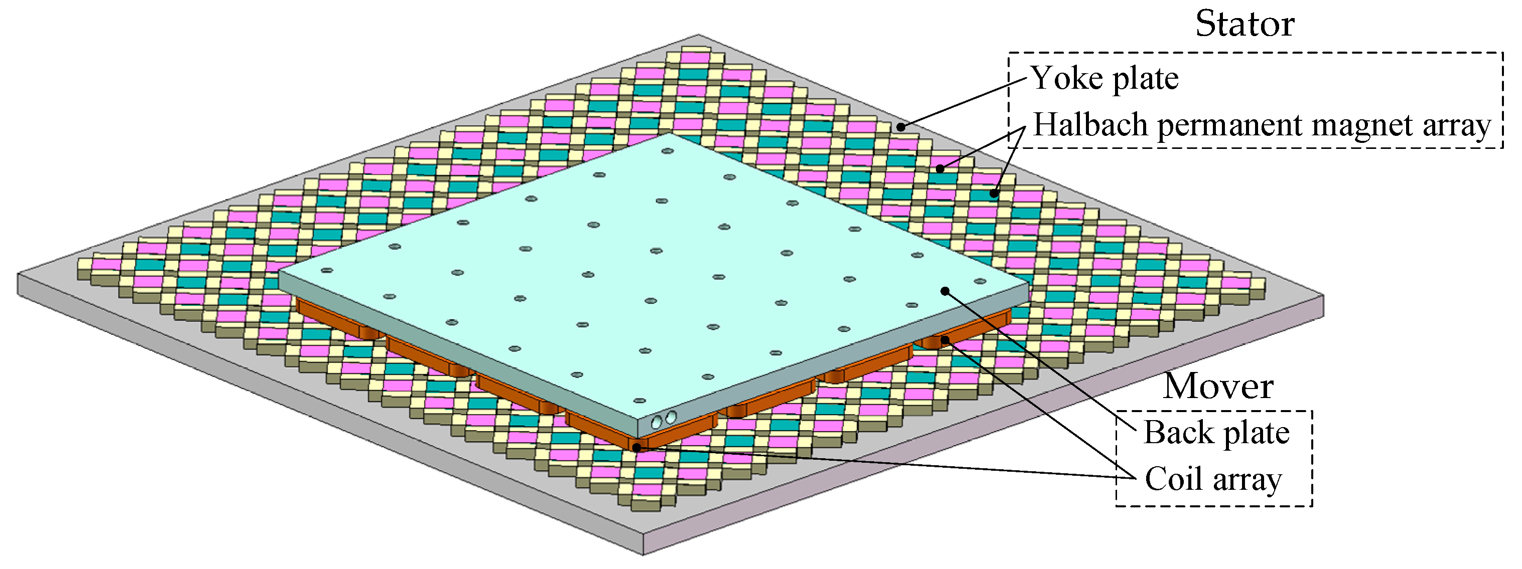
Figure 2.
Top views and A-A view of the components of a maglev planar motor: a Halbach array and a coil.
Figure 2.
Top views and A-A view of the components of a maglev planar motor: a Halbach array and a coil.

Figure 3.
Region partition.
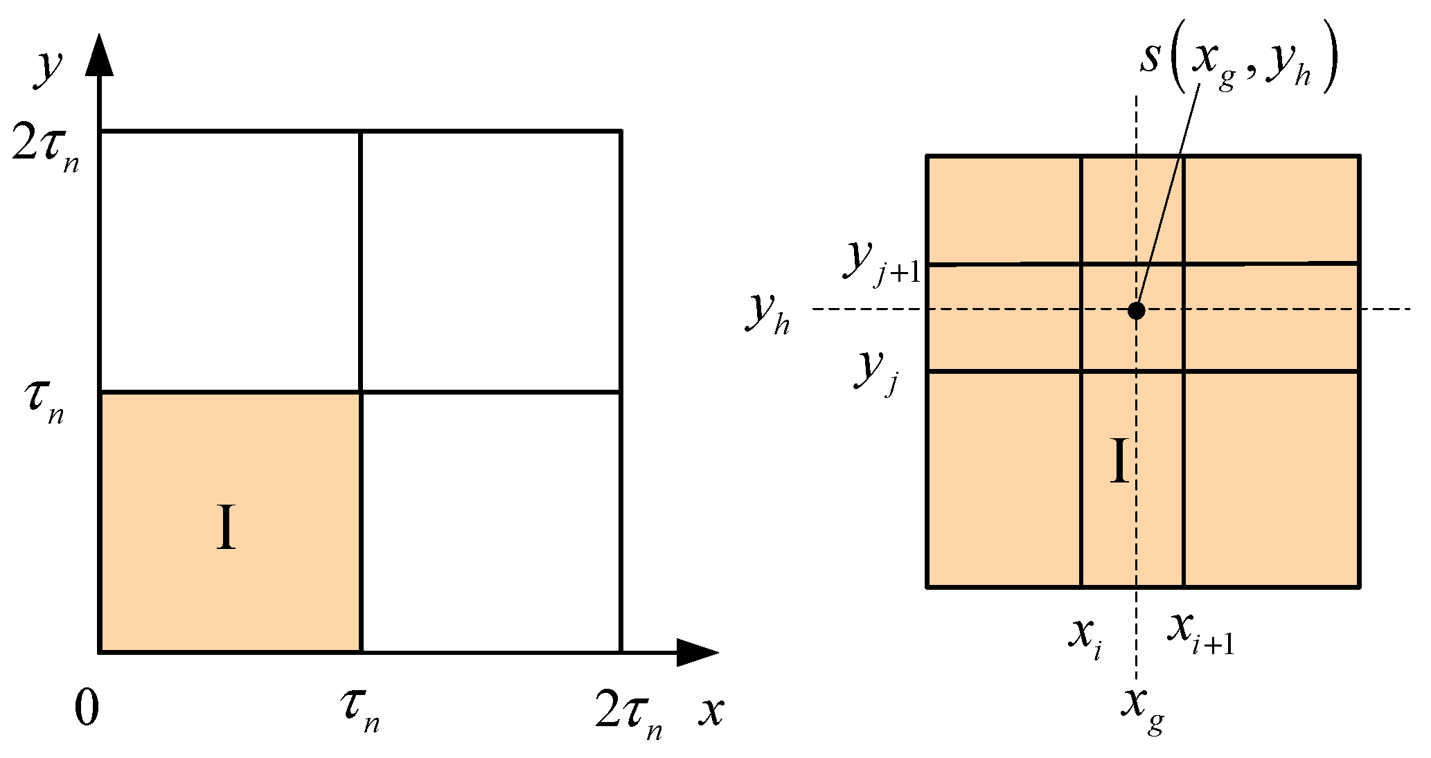
Figure 4.
Control system structure.
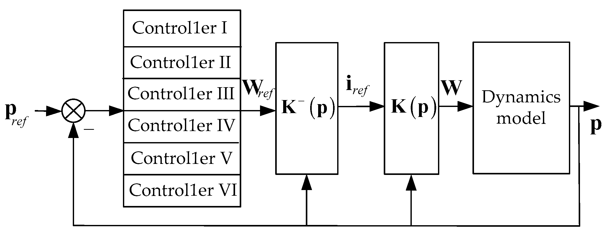
Figure 5.
Comparison of the mechanical system and the maglev system. (a) Mechanical system; (b) Maglev system.
Figure 5.
Comparison of the mechanical system and the maglev system. (a) Mechanical system; (b) Maglev system.

Figure 6.
Structure diagram of PID controller.

Figure 7.
Force and torque errors between analytical method and FEM.
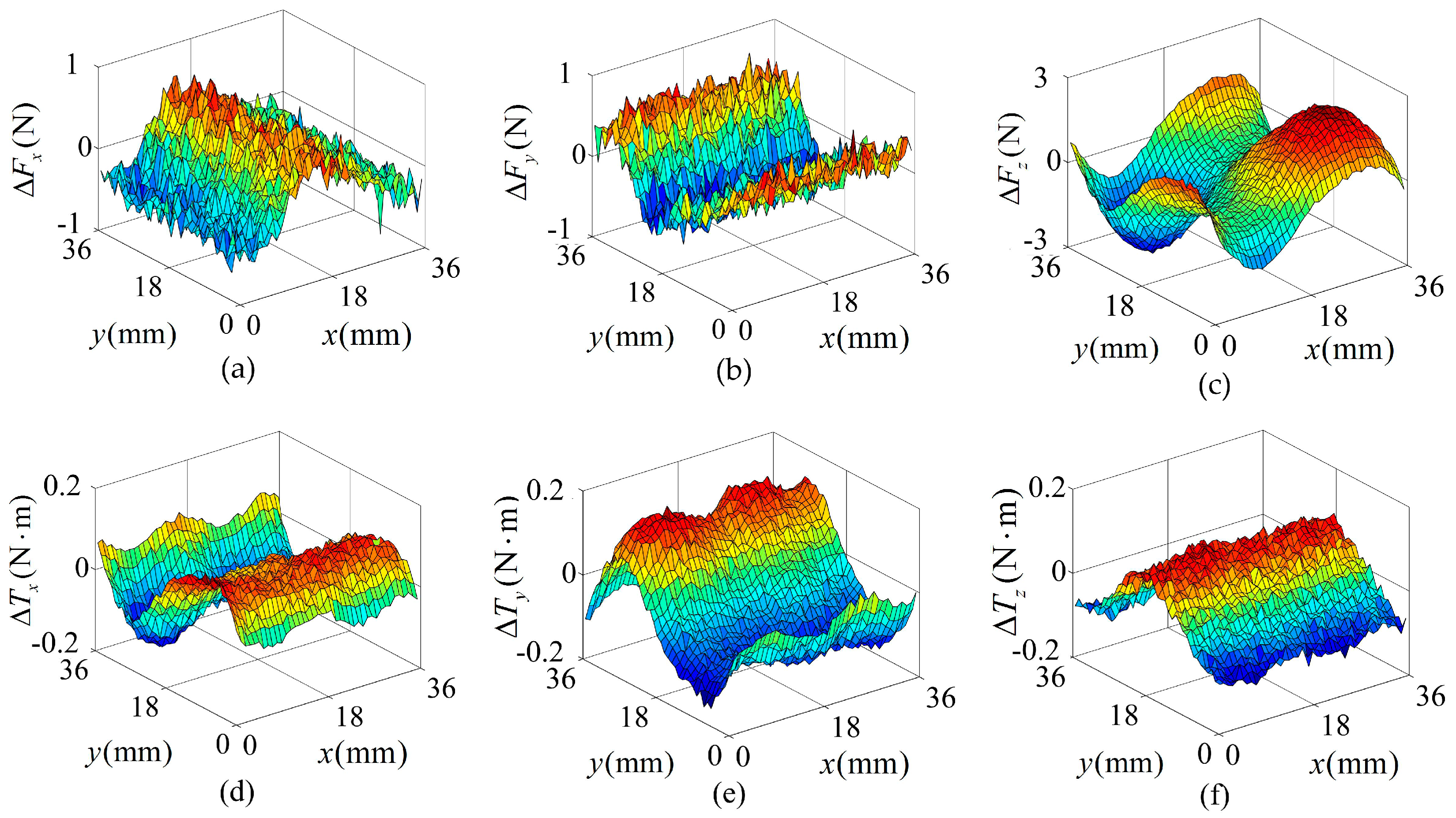
Figure 8.
Force and torque errors between interpolation method and FEM.

Figure 9.
Displacement curve of the control system based on the analytical method.
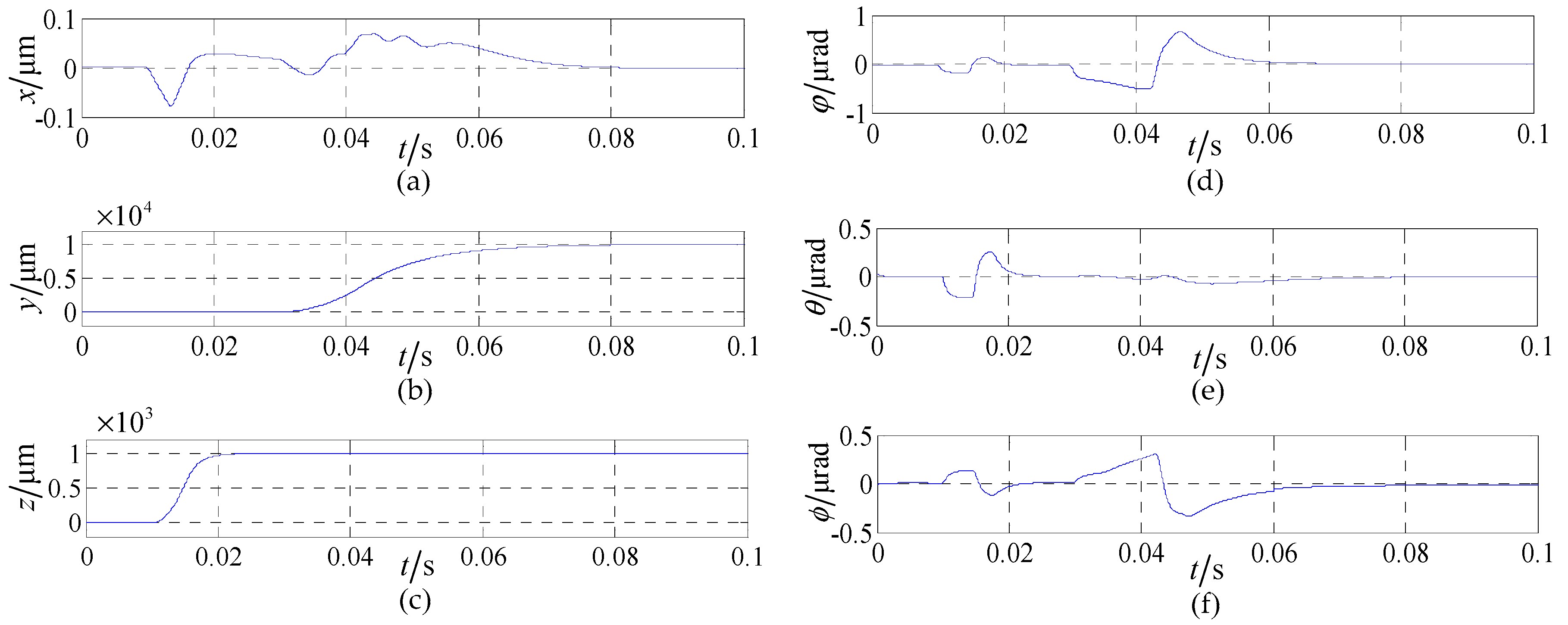
Figure 10.
Displacement curve of the control system based on the interpolation method.

Figure 11.
Force and torque curve of the control system based on the analytical method.

Figure 12.
Force and torque curve of the control system based on the interpolation method.
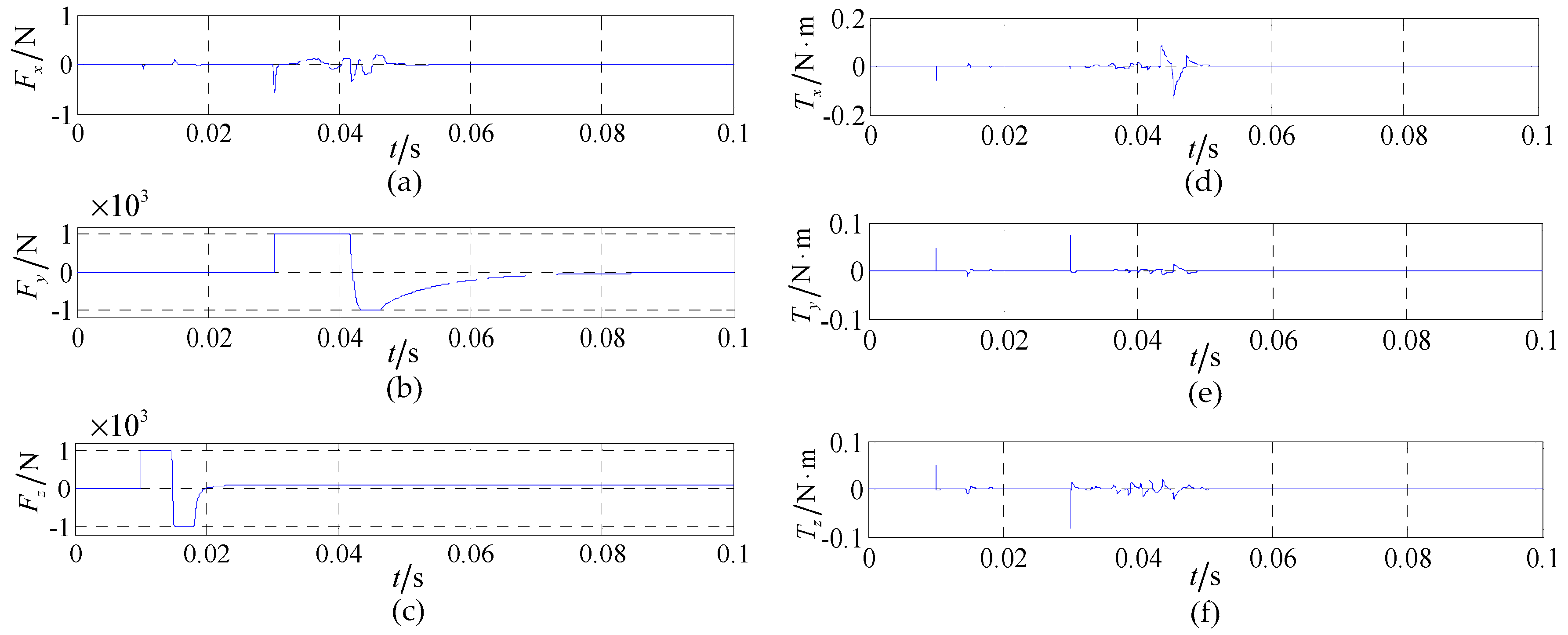
Figure 13.
Forces /torques of a coil in FEM, analytical method and interpolation method.
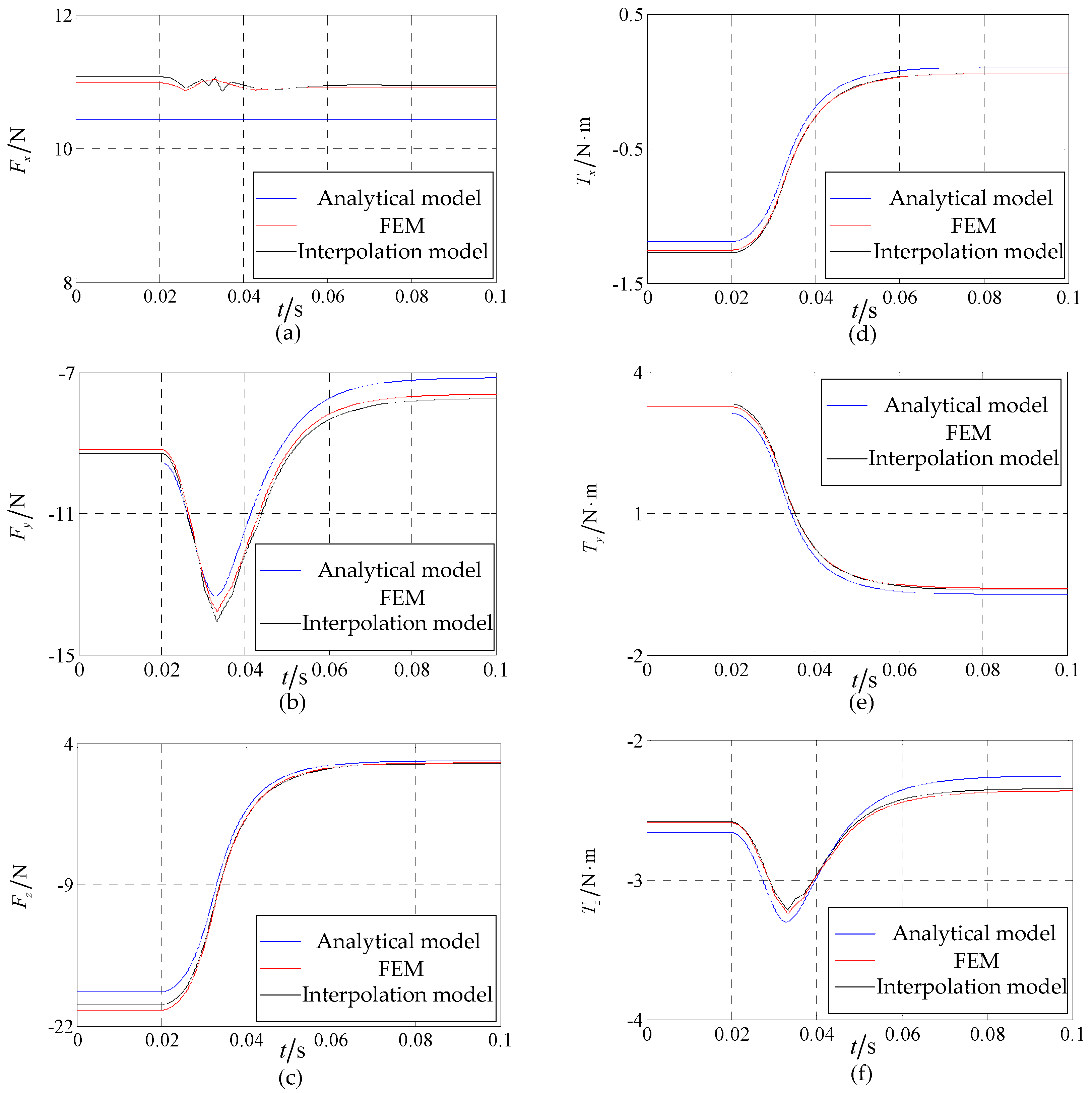
Figure 14.
Program running time analysis. (a) Real-time control platform based on NI PXI-1042Q; (b) Results of the program running time.
Figure 14.
Program running time analysis. (a) Real-time control platform based on NI PXI-1042Q; (b) Results of the program running time.


Table 1.
Main parameters of the planar motor.
| Symbol | Quantity | Value |
|---|---|---|
| τn | pole pitch | 17.7 mm |
| wc | coil width | 11.8 mm |
| hc | coil height | 10 mm |
| hm | permanent magnet thickness | 20 mm |
| h | air gap | 1 mm |
| lc | coil length of the straight coil segment | 53.1 mm |
| Bz | magnetic flux density vertical component | 0.81 T |
| Nc | number of turns | 218 |
| m | mover mass | 20 kg |
| Ix | x-axis moment of inertia | 0.268 kg·m2 |
| Iy | y-axis moment of inertia | 0.268 kg·m2 |
| Iz | z-axis moment of inertia | 0.533 kg·m2 |
| g | acceleration of gravity | 9.8 m/s2 |
Table 2.
Computation time of FEM, interpolation method and analytical method.
| Method | Time |
|---|---|
| FEM | 1 h |
| analytical method | 200 μs |
| interpolation method | 200 μs |
© 2017 by the authors. Licensee MDPI, Basel, Switzerland. This article is an open access article distributed under the terms and conditions of the Creative Commons Attribution (CC BY) license (http://creativecommons.org/licenses/by/4.0/).
Share and Cite
MDPI and ACS Style
Xing, F.; Kou, B.; Zhang, L.; Yin, X.; Zhou, Y. Design of a Control System for a Maglev Planar Motor Based on Two-Dimension Linear Interpolation. Energies 2017, 10, 1132. https://doi.org/10.3390/en10081132
AMA Style
Xing F, Kou B, Zhang L, Yin X, Zhou Y. Design of a Control System for a Maglev Planar Motor Based on Two-Dimension Linear Interpolation. Energies. 2017; 10(8):1132. https://doi.org/10.3390/en10081132
Chicago/Turabian StyleXing, Feng, Baoquan Kou, Lu Zhang, Xiangrui Yin, and Yiheng Zhou. 2017. "Design of a Control System for a Maglev Planar Motor Based on Two-Dimension Linear Interpolation" Energies 10, no. 8: 1132. https://doi.org/10.3390/en10081132
Note that from the first issue of 2016, this journal uses article numbers instead of page numbers. See further details here.