A Quantification Index for Power Systems Transient Stability

Abstract

In order to assess the reliability of power systems, transient stability simulations must be conducted in addition to steady state study. The transient stability component of reliability studies usually involves extensive simulations generating large amounts of data to be analyzed. Conventional stability analysis relies on a visual examination of selected simulation data plots to classify the severity of disturbances. This conventional examination, which aims to compare the simulations results to established performance criteria, is not comprehensive, is time consuming and prone to subjective interpretation. This paper presents a quantification method for power system performance evaluation. It applies a range of criteria such as rotor angle separation, loss of source, damping, and voltage sag directly to the simulation data files to achieve a more efficient and objective stability assessment. By using stability modules, the proposed method evaluates the performance of every fault location, numerically, by providing a local stability index, as well as an overall global stability index. The method also provides an evaluation of dispatches and their impacts on system stability. The IEEE 39-bus test system and the Northeast Interconnection Power System were used to show the results of this method. This method will free engineers from tedious, time-consuming and error-susceptible offline visual analysis and yield significantly quantified results.

1. Introduction

Power system stability simulation plays an extremely important role in reliability assessment and performance analysis. Transmission planning studies often require stability simulations to verify a power system’s compliance to electric power industry reliability standards and propose upgrade or mitigation options if reliability violations are identified. Examples of transmission planning studies include interface transfer limit studies, renewable interconnections and Bulk Power System (BPS) classification testing [1]. For example, in North America, the studies are conducted in compliance with the rules and guidelines of the local regional transmission organizations (RTO) or Independent System Operator (ISO), regional coordination councils such as Northeast Power Coordinating Council (NPCC), and the North American Reliability Corporation (NERC). Usually, a stability study requires many simulations to achieve credible results. For example, a recent study to conduct BPS testing for an RTO required more than a thousand simulations. The traditional screening evaluation of simulation results, using time-consuming visual examination, which is widely applied in the power industry. However, it is not the most efficient and consistent way to deal with large number of simulation results. This reduced efficiency is somewhat increased by overlooking simulation results (using engineering judgment, not all buses or locations are monitored and examined). Therefore, screening evaluations using visual examinations are not comprehensive.

The current NERC reliability standards [2] require the utilities to perform stability assessments for topology changes and upgrades in their territories. Since system upgrades are occurring more frequently, the NERC requirement significantly increases the number of transmission studies and associated stability data analysis. Reference [3] discussed the transient stability simulation requirements in the NERC reliability standard [2] and proposed automatically identifying transient stability violations based on the established criteria. It is obvious that the visual examination of the simulation data, presented in graphic format, could only cover a limited portion of the data received from simulations. This is because only a reduced number of parameters, selected through engineering judgment, are typically plotted and can be processed by human operators. Given that stability assessments are required in both the planning and operating phases of an electric power system, it is helpful to develop a comprehensive, quicker, and more efficient way to assess system performance. Realizing that the total number of simulations increases as the number of dispatches and contingencies are increased, the improved review method will reduce the engineering workload. Furthermore, the use of performance indices advocated in the proposed method will assist the analysis team in selecting mitigation options.

Over the last few decades, transient energy analysis using the conventional time domain simulation has been studied by several researchers. Generator stress indices were developed based on individual transient energy functions [4]. A stability index that can be used for fast determination of transient stability limits has also been derived in a hybrid method [5]. The first swing stability index was produced by incorporation of energy analysis into conventional time domain transient simulation [6]. From a practical point of view, the first swing behavior will not be sufficient to tell the whole story, stability issues might occur after few oscillations or more, because the interaction with control devices takes time to play out. Therefore, RTOs prefer to use time domain simulation to observe the system behavior from a few seconds up to 1 min after the transient stability event occurred; this is commonly applied in power system stability studies. Since the computational capacity for time domain simulation has greatly increased through the use of cloud computing [7], high performance computing [8], and parallel and distributed computing [9], the burden of performing comprehensive system simulation has largely gone unnoticed. Reference [10] has briefly introduced the methodology of quantification of transient stability assessment, however, the details of the assessment procedure was not discussed.

In this paper, a systematic power system transient stability performance quantification (TSPQ) method is proposed, which applies the existing NERC assessment criteria objectively. The procedure presented in this paper differs from our earlier work [10] by: (1) presenting a detailed performance quantification procedure; (2) redefining the stability modules included in the stability index; (3) the addition of new dispatches for the IEEE 39-bus test system case study and detailed verification of the TSPQ method; and (4) the inclusion of actual Northeast Interconnection Power System (NIPS) base cases. In summary, the system transient stability performance is characterized by a local stability index r and a global stability index R in this paper. These stability indices are developed by assessing the most common stability criteria [11], which include system angular separation [12,13], loss of source (LOS) [14], damping [15,16], and voltage sag [17]. The number of stability modules could certainly be expanded or modified to include other criteria that might be of interest for any given study. The focus of this paper is the presentation of the improved analytical methodology to a large volume of transient simulation data rather than the discussion of the detailed criteria or base case selection. The local stability index r, which quantifies the violations severity of a given contingency and system condition, can be used as a guide in the identification of system upgrade options since it offers a ranking of the offending contingencies and system conditions. The r values attribute to different fault locations (buses) and provides a useful way to visualize the effect of system configuration changes on the transient stability performance. The global stability index R is an indicator of the system strength or weakness under the given set of contingencies and dispatches. R consists of a practical mathematical implementation of the stability assessment module. It provides a rank to the selected system configuration(s) and facilitates the mitigation investigation if specific contingencies or system configurations are unacceptable.

This paper is organized into six sections. The second section reviews the stability simulation procedure, and explains the TSPQ method. The third section covers the details of each stability module in Section 2, and the proposed local and global stability index calculation. Subsequently, the fourth section discusses the IEEE-39 bus test system case study. To show the result of the TSPQ method on a real power system, Section 5 implements the TSPQ method in the Northeast Interconnection Power System (NIPS), and the results are discussed. The last section provides the conclusion of the paper.

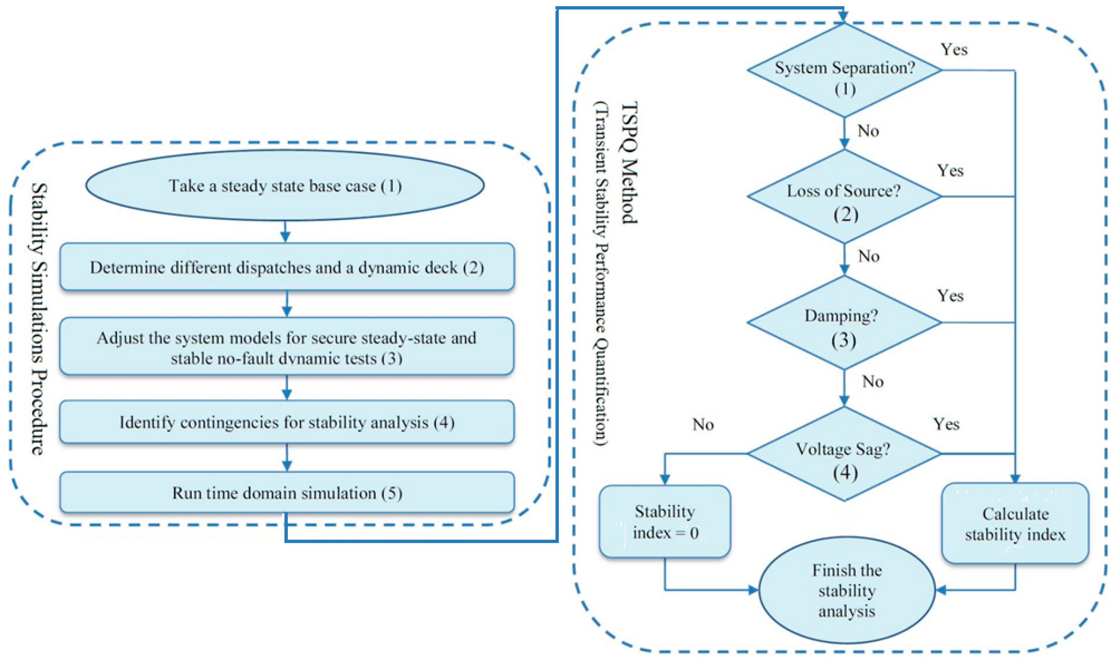
2. Overview of the Proposed Performance Quantification Procedure

Power systems are constantly undergoing changes including modifications to existing systems, the integration of renewable energy, the retirement and replacement of power plants, and upgrades to existing facilities. RTOs conduct the study for these proposed modifications, and make sure the changes do not have any adverse impact on the stability of the system. As a result, there is a sustained need for stability analysis in transmission planning and operation. Each RTO has its own procedures [18] for conducting such assessments. The diagram shown in Figure 1 includes two blocks: (1) Stability Simulation Procedure (SSP), which is used by RTOs and it illustrates the steps taken to run stability simulations; and (2) Transient Stability Performance Quantification (TSPQ) Method, which is proposed in this paper. The first block shows how a stability simulation is normally performed, and the second block shows the proposed methodology improving the existing stability criteria to form a more comprehensive stability method.

SSP is a common procedure used in the industry for stability analysis studies. The procedure is summarized in the following steps. The first step in SSP, as shown in Figure 1, the base case usually should originate from the RTO’s library of cases, with future load and enhancement predictions included. Second, a variety of generation dispatches, reflecting perceived potential stressed transfer conditions are prepared. The dynamic models of devices and facilities should be up-to-date and correct. Third, various dispatches based on the selected base case are adjusted to ensure that their steady-state is secure (no voltage or thermal violations). This can be performed by a no-fault (no-disturbance) stability test. Note that the no-disturbance [18] simulation is required to assure that the dynamic model parameters are valid. Fourth, prepare a comprehensive set of contingencies to be tested. The selection and number of base cases and contingencies are major factors in determining the length and credibility of a study. Finally, commercial transmission planning software such as Power System Simulator for Engineers (PSS/E), Positive Sequence Load Flow (PSLF), and Power World could be used for time domain simulation.

The proposed TSPQ method in this paper will provide conclusive and detailed stability study results. The method includes four stability criteria modules and a computing module that calculates the stability result index R, as shown in the right block of Figure 1. As the simulation data pass from the SSP. These modules work in the following order. First, the system separation (SS) module examines the angular stability and generation coherency; if there is a system separation (“Yes”), then the stability index is calculated, as described in Section 3.5, and the analysis process is finished. Second, if there is no system separation (“No”), the loss of source (LOS) module kicks in. LOS verifies whether there is a loss of source and if the amount of loss of source is over a pre-defined limit (“Yes”), then the stability index is calculated, and the analysis process is finished; otherwise (“No”), continue to the damping module assessment. Third, the damping module measures the oscillation of system swings during a system disturbance. If the damping result is unacceptable (“Yes”), then the stability index is calculated, and the analysis process is finished. Finally, voltage sag (Vsag) is the last assessment performed. The module is run if all of SS, LOS, and damping results for the particular contingency-dispatch combination are acceptable. If there is an unacceptable Vsag (“Yes”), then the stability index is calculated, and the analysis process is finished; otherwise, the stability index is set to 0, which means there are no stability issues. This particular logic is chosen to reduce the analysis computation time. Other processing orders for index calculations could be considered to meet specific preferences.

3. Detailed Description of TSPQ Method

The following sub-sections describe different TSPQ steps as given in the previous section.

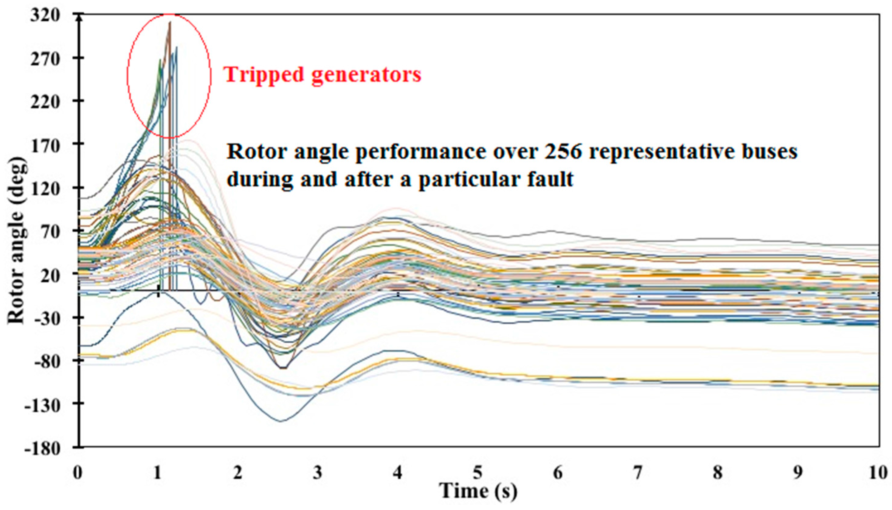
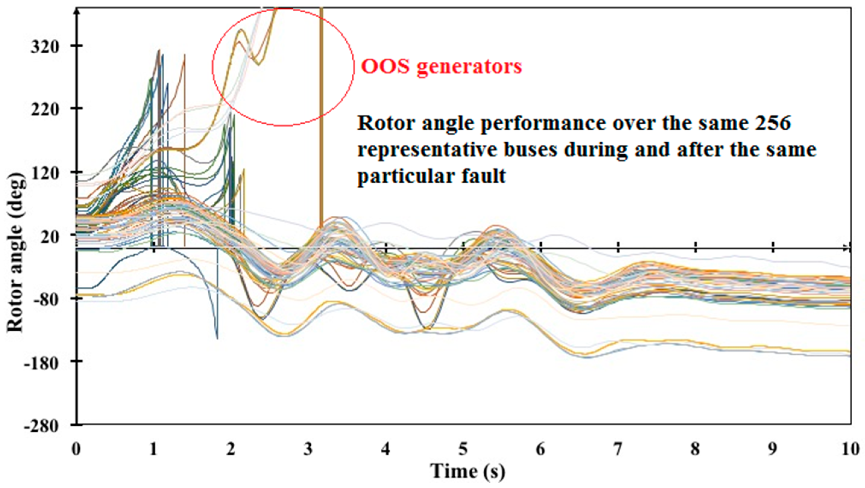
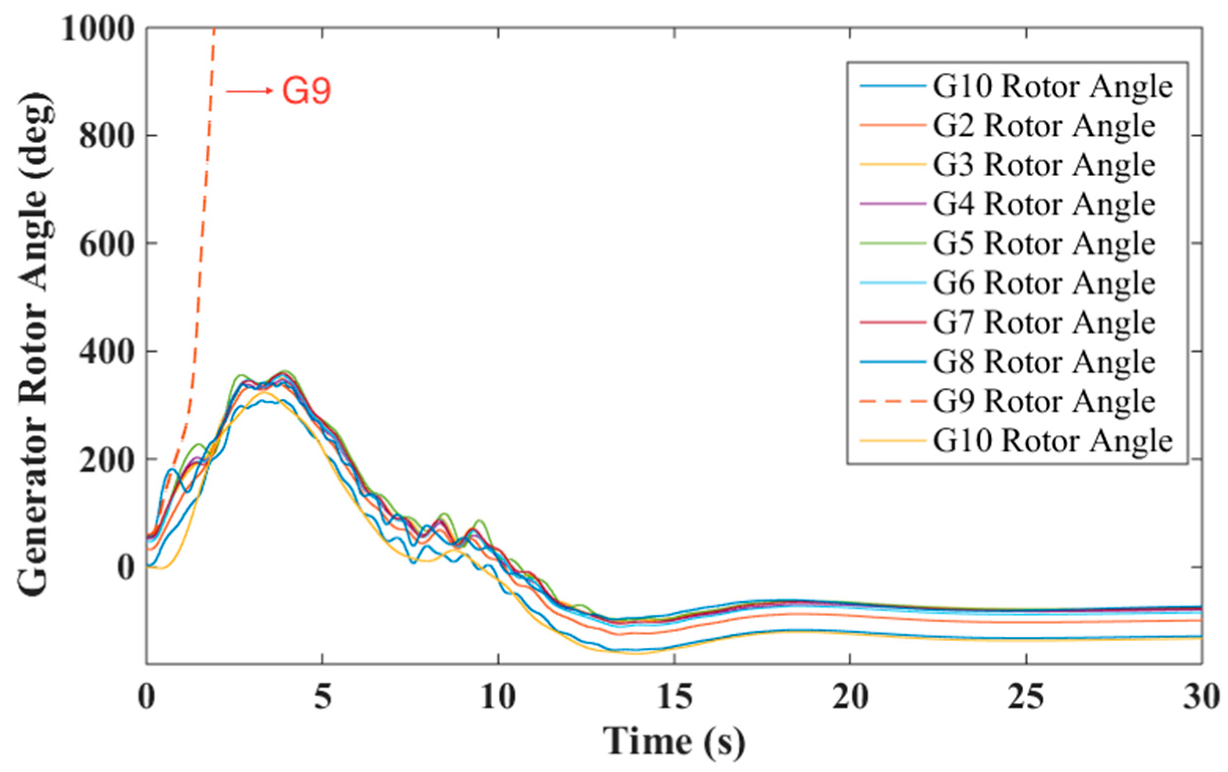
3.1. System Separation Module

Uncontrolled system separation (SS) occurs when groups of generators in a system lose synchronism. Typically, a group of generators experiences acceleration (or deceleration) which can be observed in their angular excursions relative to other generators or groups of generators. For severe contingencies, these angular excursions can lead to uncontrolled creation of islands in the system. Generators in each of these geographical pockets tend to be coherent with one another (swing together) during significant system disturbances. In general, the coherency behavior of generators can be defined using the following equations [13]:

$$\begin{array}{c}f\left(t\right)=\left|{\delta }_{ij}\left(t+\Delta t\right)-{\delta }_{ij}\left(t\right)\right|<\epsilon \\ {\delta }_{ij}\left(t\right)={\delta }_i\left(t\right)-{\delta }_j\left(t\right)\end{array}$$

(1)

where δ is the rotor angle of a generator and ε is defined as the coherency tolerance for any pair of generators (i, j).

This function uses the generator rotor angle characteristics data to identify groups of generators moving in the same direction and hence determine if the system is separating at any location. A system separation occurs if at least two groups of generators are moving in opposite directions (one group is accelerating relative to the other). This typically means that the generators in one of the groups are going out of step (OOS). OOS generators are characterized by the large angular excursions and steep slopes of their angular characteristics.

The SS module is a binary function defined as:

$$f_1=\{\begin{array}{ll}0,& \hspace{1em}\mathrm{if} \mathrm{Equation} \left(1\right) \mathrm{is} \mathrm{true}\\ 1,& \hspace{1em}\mathrm{otherwise}\end{array}$$

(2)

If all generators are coherent, then the SS module assigns a binary number 0 to represent no separation; otherwise, 1 is assigned to f₁ for separation.

3.2. Loss of Source Module

Loss of source (LOS) is defined as the loss of generating units as the result of “falling out of step (OOS)” with the rest of the system, loss of synchronism, or being tripped by an overspeed relay. This function evaluates the amount of generation (MW) loss due to two reasons: generators tripping and generators going OOS. Tripped generators are further classified into two categories: generators tripped as part of the fault-clearing process, and generators tripped due to system performance. OOS generators are identified by large angular excursions and steep slopes of their rotor angle data. Tripped generators are identified by a discontinuity in their rotor angle data (a property of the generator model). Some generator models (non-rotating generators) report the last measured angle as a constant value, while other models (rotating generators) report a zero value, for the remainder of the simulation. The allowable magnitude of such losses, $P_{Limi{t}_C}$, for a reliable generation dispatch depends on the contingency considered. Thus, the total loss, $P_{loss}$, for a reliable generation dispatch under the varying system conditions could be defined as:

$$P_{loss}={\displaystyle \sum }_{i=1}^n{P}_{i_{loss}}<P_{Limi{t}_C}$$

(3)

$P_{Limi{t}_C}$ is specified in the reliability requirements and varies with different categories of contingencies. Normal contingencies must not trigger any generation loss, except the tripping of generators as a necessary part of the contingencies. Units tripped in this way are not included in the loss of source tally since they do not constitute a significant adverse impact condition [19]. The infrequent extreme contingencies, very expensive to mitigate, allow a maximum loss of generation inside a specific region. Similar rules apply in other RTO territories. This maximum is determined from operating experience and the availability of replacement power from adjacent regions.

Finally, LOS module, similar to SS module, assigns a binary number to module, as:

$$f_2=\{\begin{array}{ll}0,& \hspace{1em}\mathrm{if} \mathrm{Equation} \left(3\right) \mathrm{is} \mathrm{true}\\ 1,& \hspace{1em}\mathrm{otherwise}\end{array}$$

(4)

If the amount of loss of source is within the given limit, then the LOS module assigns a binary number 0 to represent no violation situation; otherwise, 1 is assigned to f₂ for violation situation.

3.3. Damping Module

Damping is a measurement of the oscillation decay of the parameters associated with swings of synchronous machines subjected to a system disturbance. The oscillation often happens in a group of generators in a region. Reducing the power transfer or adding/tuning the Power System Stabilizers (PSS) appropriately could often help to attenuate the oscillation. The damping assessment can be performed by analyzing angle, voltage, frequency, interface power flow, apparent impedance and individual generator electrical and mechanical power data, from generator and transmission buses. However, angles and voltages are typically used to examine the health of the system, because all other factors are related to them.

An example for the determination of acceptable damping criteria is described in the ISO New England document [15]. The following exponential decay equation demonstrates the acceptable relationship:

$$f\left(t\right)=1-e^{-\zeta {\omega }_{n}t}\ge 53\%$$

(5)

where ζ = 0.03, and ω_n is the natural frequency of oscillation in Hz. Time domain analysis is used for a sufficient time (up to 30 s) of transient stability simulation. To pass the damping test, a 53% reduction in the magnitude of the oscillation must be observed over four periods of the oscillation, from the point where only a single mode of oscillation remains. Simulation data of all system state quantities (rotor angle, voltage, interface transfers, etc.) should be analyzed to ensure that adequate system damping is observed. The normalized damping severity is defined in Equation (6).

$$f_3=\{\begin{array}{cc}\hfill 0,& \hspace{1em}\mathrm{if} \mathrm{Equation} \left(5\right) \mathrm{is} \mathrm{true}\hfill \\ \hfill \frac{\left|f\left(t\right)-53\%\right|}{53\%},& \hspace{1em}\mathrm{otherwise}\hfill \end{array}$$

(6)

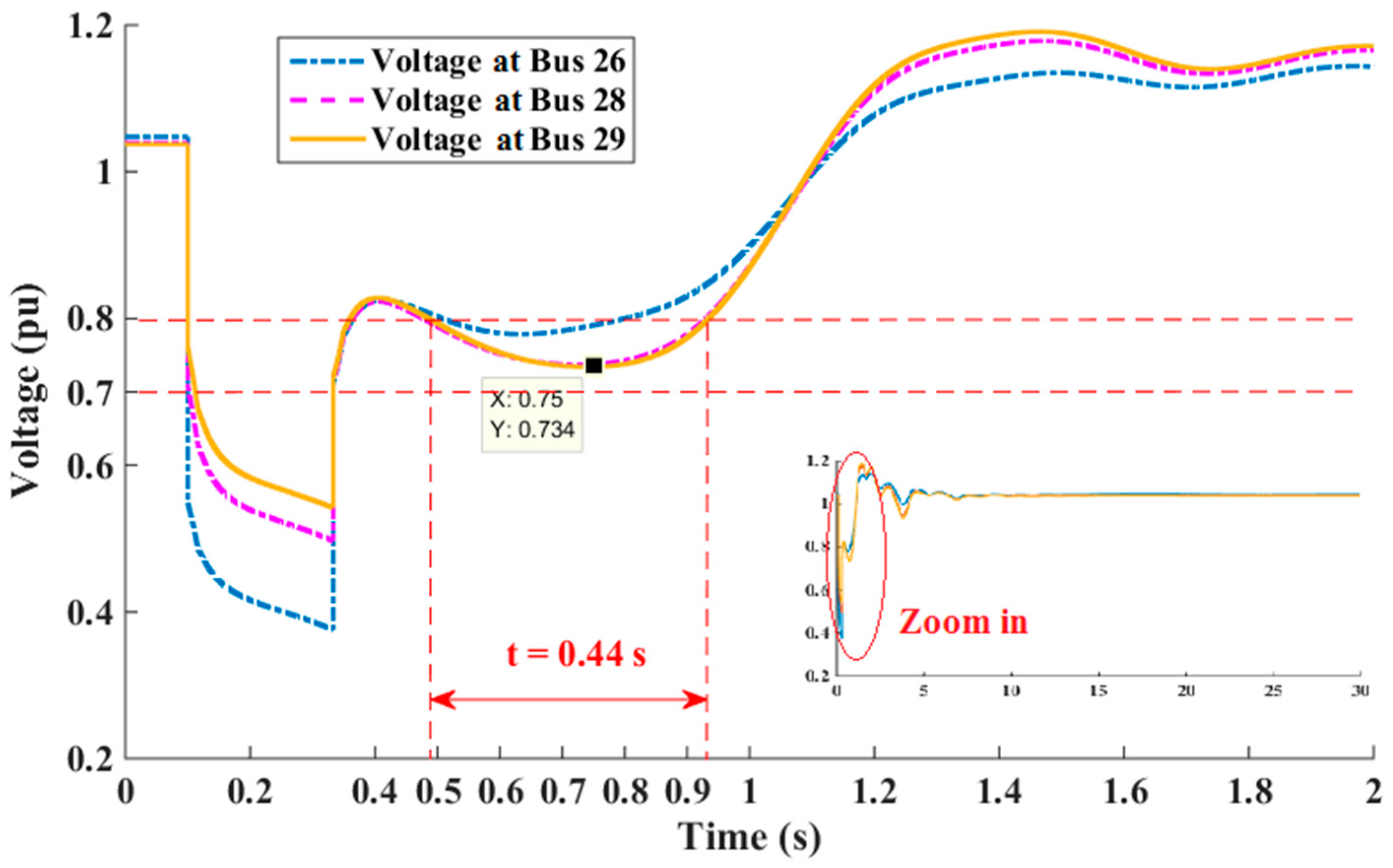
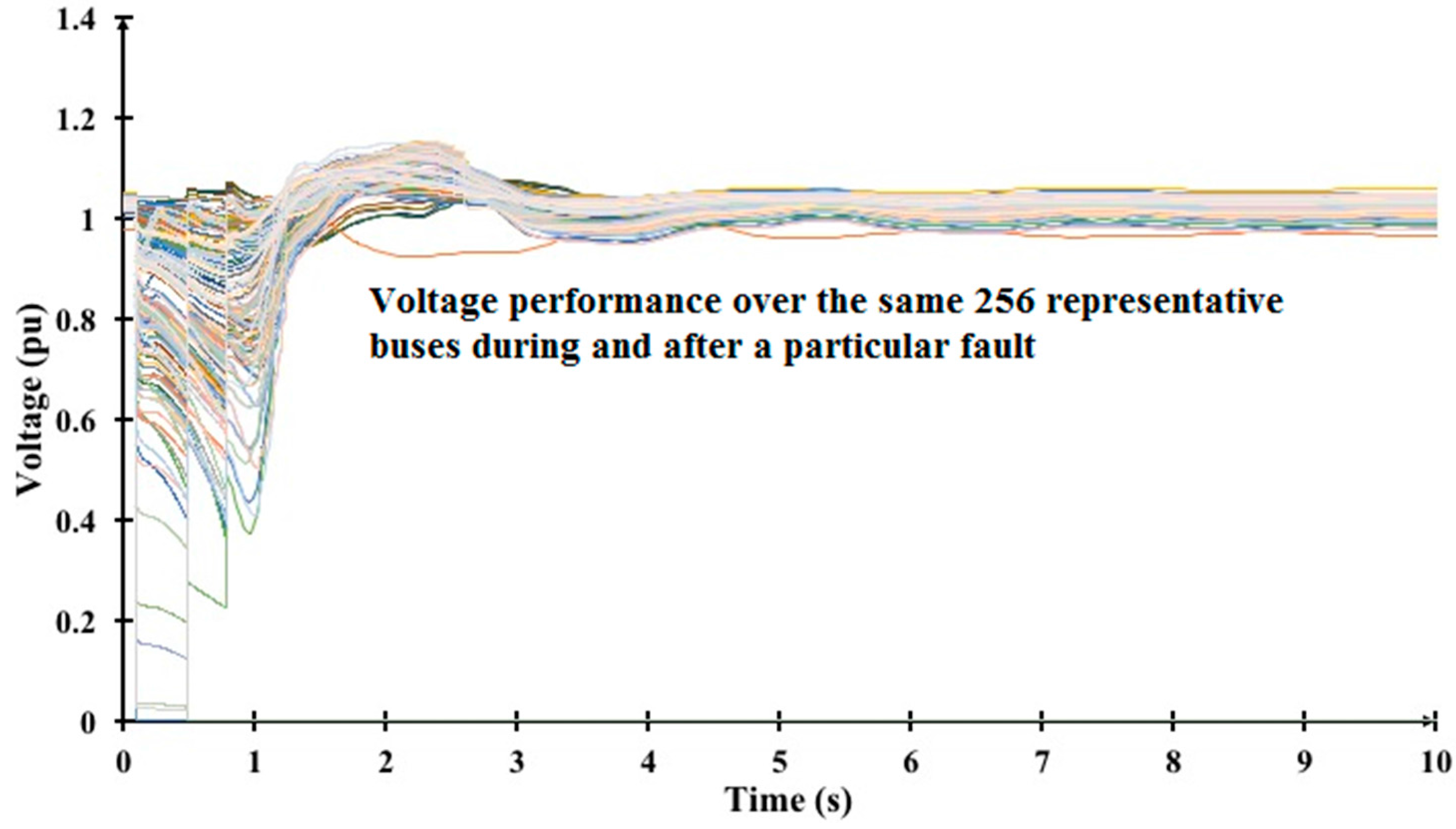
3.4. Voltage Sag Module

A system fault causes voltages at nearby buses to be temporarily depressed to low levels until the fault is cleared. Voltage sags are unavoidable and under certain conditions, they are acceptable. After a stable fault is cleared, the system oscillates on its way to the post-fault state and the voltages tend toward the post-fault steady-state level. Following the fault clearing, the “back-swing”, a significant transient voltage sag caused by the call for post-fault accelerating power, is superposed on transient oscillation. The limits set for this post-fault voltage sag characteristic, described in [17], are the basis of the Voltage Sag Module: the minimum post-fault voltage sag must remain above 70% of nominal voltage and must not exceed 250 milliseconds below 80% of nominal voltage within 10 s following a fault. The following Equations (7)–(9) demonstrate the relationships for voltage sag time delay failure, voltage sag low limit failure and voltage not above failure, respectively.

$$0.7 \mathrm{pu}<f\left(t\right)\le 0.8 \mathrm{pu} \& t_{0.8}>0.25\mathrm{s}$$

(7)

$$f\left(t\right)\le 0.7 \mathrm{pu}$$

(8)

$$0.75 \mathrm{pu}\le f\left(t\right)\le 0.8\mathrm{pu}$$

(9)

where t_0.8 is the time delay of the voltage sag below 0.8 pu. Equations (7)–(9) check if the voltage sag function f(t) violates the magnitude and time limitation. If Equation (7) or Equation (8) or Equation (9) is true, then the voltage sag severity is defined as:

$$f_4=\{\begin{array}{cc}\hfill 0,& \hspace{1em}\mathrm{if} \mathrm{neither} \mathrm{Equations} \left(7\right),\left(8\right) \mathrm{or} \left(9\right) \mathrm{is} \mathrm{true}\hfill \\ \hfill 1-f_{worst}\left(t\right),& \hspace{1em}\mathrm{otherwise}\hfill \end{array}$$

(10)

where f_worst(t) is the worst voltage sag value found by comparing all voltage sag values.

3.5. Stability Index R Calculation

The stability index R is the sum of the stability assessment module values, computed from the simulation results of specific design contingencies, system topology, and generation dispatch of the power system. The performance of a system could thus be quantified through this index, which is expressed as:

$$\mathit{R}={\displaystyle \sum }_{i=1}^n{r}_{Bu{s}_i}$$

(11)

where n is the bus number where contingencies occur. $r_{Bu{s}_i}$, defined by Equation (12), is the cumulative value of all the test modules for all the contingencies applied to a given bus. It is considered the local stability performance index for the particular system configuration. $r_{Bu{s}_j}$ is calculated by using the below Equation:

$$r_{Bu{s}_i}={\displaystyle \sum }_{j=1}^m\left(\begin{array}{c}\left[c_{j1} c_{j2} c_{j3} c_{j4}\right]\left[\begin{array}{c}{f}_1\\ \begin{array}{c}{f}_2\\ f_3\end{array}\\ f_4\end{array}\right]\\ C_{j}F\end{array}\right)={\displaystyle \sum }_{j=1}^m\left(c_{j1}{f}_1+c_{j2}{f}_2+c_{j3}{f}_3+c_{j4}{f}_4\right)$$

(12)

where m is number of contingencies at Bus_i being analyzed in the assessment. c_j1f₁, c_j2f₂, c_j3f₃, c_j4f₄ are the values assigned by the modules algorithms for contingency C_j. For example, if contingency C_j fails the f₁ assessment, then c_j1f₁ equals 1, otherwise it equals 0.

For this proposed procedure, a specific practical priority was assigned to the testing modules Although another testing sequence could have been adopted for ranking the performance of the various system configurations under the selected contingencies, this approach increases the efficiency and speed of the analysis by halting the test of a contingency when its effect on the system is clearly unacceptable. The logical analysis vector for the functions follows the higher to lower priority order for modules f₁, f₂, f₃, f₄, and can be expressed in condensed form as:

$$F_L=\left[\begin{array}{c}{f}_1\\ \begin{array}{c}0\\ 0\end{array}\\ 0\end{array}\right]$$

(13a)

$$F_L=\left[\begin{array}{c}0\\ \begin{array}{c}{f}_2\\ 0\end{array}\\ 0\end{array}\right]$$

(13b)

$$F_L=\left[\begin{array}{c}0\\ \begin{array}{c}0\\ f_3\end{array}\\ 0\end{array}\right]$$

(13c)

$$F_L=\left[\begin{array}{c}0\\ \begin{array}{c}0\\ 0\end{array}\\ f_4\end{array}\right]$$

(13d)

where Equation (13) includes four sub-Equations (13a)–(13d). Equation (13a) represents the case when f₁ is analyzed first, and if f₁ fails, then f₂, f₃, and f₄ are not considered for analysis; Equation (13b) represents a case when f₁ and f₂ are analyzed, only f₂ fails, and therefore there is no need to analyze f₃ and f₄; Equation (13c) represents a case when f₁, f₂ and f₃ are analyzed, only f₃ fails, and then f₄ is skipped; and Equation (13d) represents a case when f₁, f₂, f₃, and f₄ are analyzed and only f₄ fails.

Usually, the SS and LOS modules are considered as go-no-go events so they are assigned binary values, as shown in Equations (2) and (4). The damping and Vsag events, however, occur in a range of severity, from acceptable to highly unacceptable. Therefore, they are more appropriately assessed on an analog scale and are assigned numerical analog merit values, as shown in the detailed expressions of Equations (6) and (10). The goal of power system study using the proposed analysis methodology is to rank the selected system configurations and to facilitate the mitigation investigation if specific contingencies or system configurations are unacceptable.

Various stability assessment categories require different criteria functions. For instance, for a normal contingency assessment, all four modules are considered, but for a Bulk Power System (BPS) assessment, Vsag module is not considered.

The above illustration is for a single dispatch. Equation (11) expresses the global stability index assessment result for a given system configuration. Multiple system configuration simulations can be executed through parallel computing, using the same process. The inclusion or exclusion of certain modules can be determined using the RTO’s reliability standards. This would necessitate a corresponding number of additional contingencies C matrix and modules matrix F in Equation (12).

4. IEEE 39-Bus Test System Case Study and Verification

The purpose of this case study is to demonstrate the proposed TSPQ method, to verify the performance of each module, and to interpret the r and R stability index values.

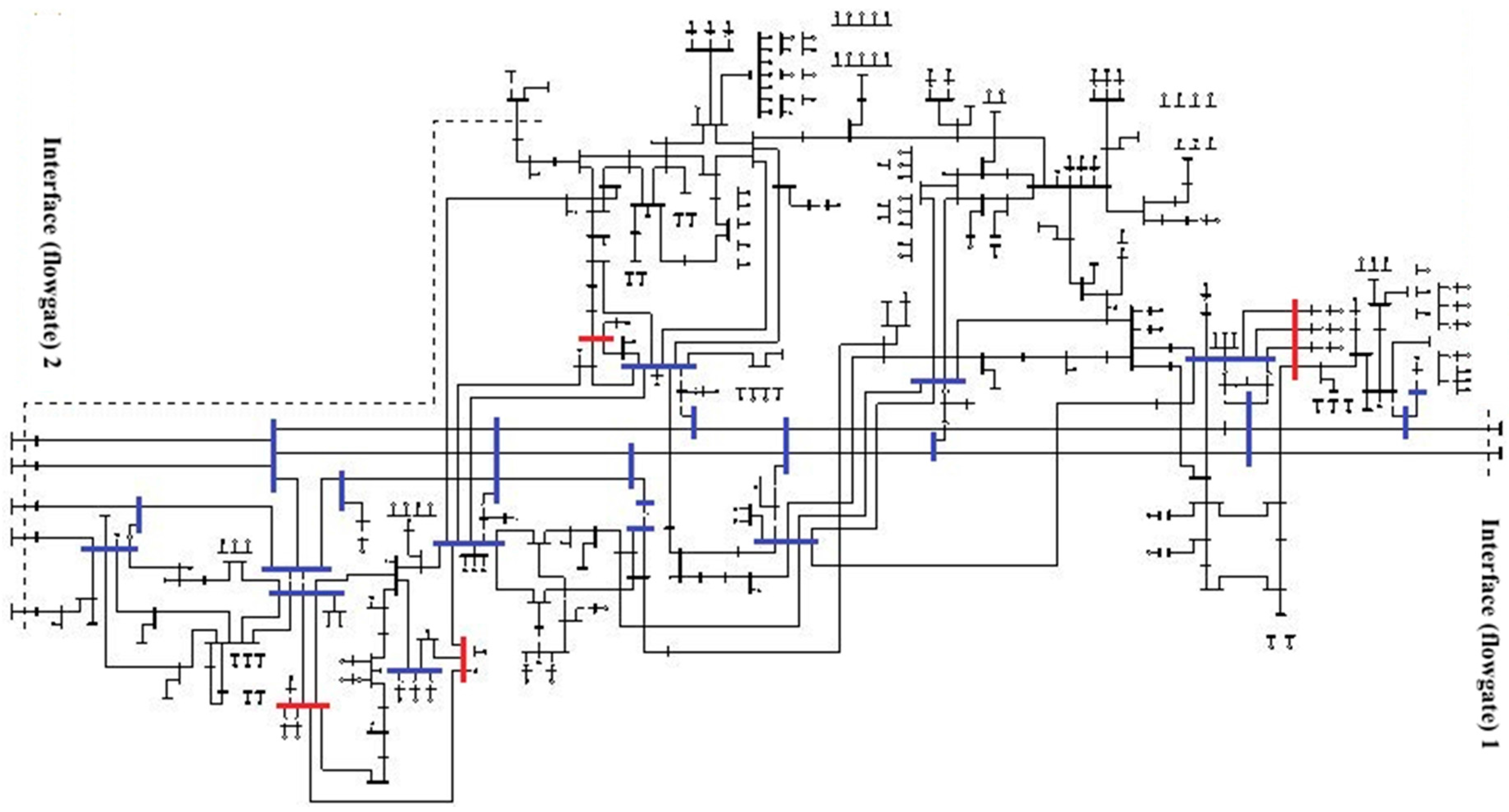
4.1. IEEE 39-Bus Test System

This case study uses the IEEE 39-bus test system to demonstrate the above methodology, and the detailed analysis strategy. The IEEE 39-bus test system is well known as the 10-machine New England Power System, with each depicted generator (Figure 5) representing a set of generators. All power flow data and generator model data are obtained from [20] and [21]. In addition to the above data, dynamic models including exciters and governors are added for each generator, and they are tuned for this transient stability study. PSS/E is utilized for the simulation to generate the data set for TSPQ method. Initialization of the dynamic models is carried out to make sure they are capable of successful “flat starts” [18] for each dispatch, which was mentioned in Section 2 in the description of the stability simulation procedure. The simulations are run for a duration of 30 s in this paper.

4.2. Contingencies and Dispatches

The main objective of the case study is to test the proposed TSPQ method. Data from three phase faults is generated for the test. The faults have clearing times ranging from 1 to 20 cycles, applied at each bus in the system (including generator terminal buses and load buses). A total of 780 simulations were thus performed for each base case. Six base cases with different generators dispatches, summarized in

Table 1. IEEE 39-bus system dispatches.

	D0 (MW)	D1 (MW)	D2 (MW)	D3 (MW)	D4 (MW)	D5 (MW)
G1	998	999.5	994	994.3	996.8	997.2
G2	573	573	573	573	673	673
G3	650	550	450	350	750	812.5
G4	632	632	632	632	732	790
G5	508	508	508	508	608	600
G6	650	650	650	650	750	812.5
G7	560	560	560	560	660	845
G8	540	540	640	640	640	1000
G9	830	933	933	933	930	1000
G10	250	250	250	350	350	500
Total MW in each dispatch
	6191	6195.5	6190	6190.3	7089.8	8030.2

, were tested to generate a variety of performance violations. In order to verify the TSPQ algorithms, each dispatch gives the power generation of system generators. D₀ is the original dispatch (base case) with all ten generators’ real power values shown in Table 1 below; D₁, D₂ and D₃ are dispatches based on D₀ by adjusting the generated power of G3, G8, G9, and G10, while keeping the whole system’s real power at the same level (6190 MW). Dispatches D₄ and D₅ have total system real power and load increased by 14.5% and 29.7% respectively relative to D₀. D₅ is obtained by pushing all generators to their real power limits. In Table 1, the shaded areas indicate dispatches with significant changes compared to dispatch D₀.

4.3. TSPQ Method Results

The stability simulations performed for the different contingencies and dispatches provided a diversified data set for testing the TSPQ method. The f₁, f₂, f₃, and f₄ output values of the SS, LOS, damping and Vsag modules were computed using expression (13), and then aggregated to yield the stability indices.

4.3.1. Results for Dispatch D₀

To demonstrate the TSPQ method for dispatch D₀, a three-phase fault was applied to Bus 2. The SS, LOS, damping, and Vsag module results are listed in

Table 2. Simulation results at bus 2 for dispatch D₀.

Fault Location	Clearing Time (Cycles)	SS (f1)	LOS (f2)	Damping (f3)	Vsag (f4)
Bus2	1	0	0	0	0
Bus2	2	0	0	0	0
Bus2	3	0	0	0	0
Bus2	4	0	0	0	0
Bus2	5	0	0	0	0
Bus2	6	0	0	0	0
Bus2	7	0	0	0	0
Bus2	8	0	0	0	0
Bus2	9	0	0	0	0
Bus2	10	0	0	0	0
Bus2	11	0	0	0	0
Bus2	12	0	0	0	0
Bus2	13	0	0	0	0
Bus2	14	0	0	0	0.266
Bus2	15	0	0	0	0.344
Bus2	16	1	N/A	N/A	N/A
Bus2	17	1	N/A	N/A	N/A
Bus2	18	1	N/A	N/A	N/A
Bus2	19	1	N/A	N/A	N/A
Bus2	20	1	N/A	N/A	N/A
rBus2 = 5.61

. For example, Table 2 shows that for the simulations with a fault clearing time (FCT) less than 14 cycles (1st–13th rows), none of the modules (f₁, f₂, f₃, and f₄) fails, as indicated by a “0”. Increasing FCT to 14 and 15 cycles will result in voltage sags, as indicated in Table 2, but not system separation or loss of source. An analysis of the voltage performance for the 14-cycle fault shows that only buses 26, 28 and 29 experience voltage sags, as shown in Figure 2. Among the three buses, bus 29 had the worst sag of 0.734 pu (black square data-tip shown in Figure 2) among all voltage sags. According to Equations (7) and (10), f₄ is evaluated to be 0.266 pu, shown in row 14th and column Vsag of Table 2. For the 15-cycle FCT, f₄ can be calculated in the same manner resulting in 0.344 pu.

Increasing the FCT further to 16 cycles, generator G9 at bus 38 will go out-of-step (detected by the System Separation module), hence, f₁ = 1. Figure 3 shows the graphical representation of the angle excursion of G9 and its separation from the other nine generators. Note that Figure 3 has been introduced here to clarify the TSPQ analytical process. It provides a validity check of the module performance but is not needed or used in the TSPQ analysis methodology. All other generator rotor angles, except G9’s, are coherent in the same oscillation pattern, and settle down in a 30 s simulation. Since system separation has higher priority, as indicated in Section 3, the LOS module (f₂) and others do not need to be considered, indicated by N/A in Table 2. Given that the 16-, 17-, 18-, 19- and 20-cycle FCT three phase faults caused the system to experience system separation, N/As are presented in the rest of LOS, damping, and Vsag columns in Table 2.

The local stability index (r_Bus2) for bus 2 is 5.61, as shown in Table 2, which is the summation of f₁, f₂, f₃, and f₄ values in Equation (12). Note that for cycles 1 to 20, the fault clearing time range, with a 1 cycle step, was selected to provide a wide variety of stability performance simulation results for the TSPQ methodology test. Although reasonable, these clearing times are not meant to reflect actual protection practices. Local stability indices for all other buses were calculated in the same manner for D₀. The global stability index R for dispatch D₀ was calculated using Equation (11). A similar procedure was followed to calculate the local and global stability indices for other dispatches.

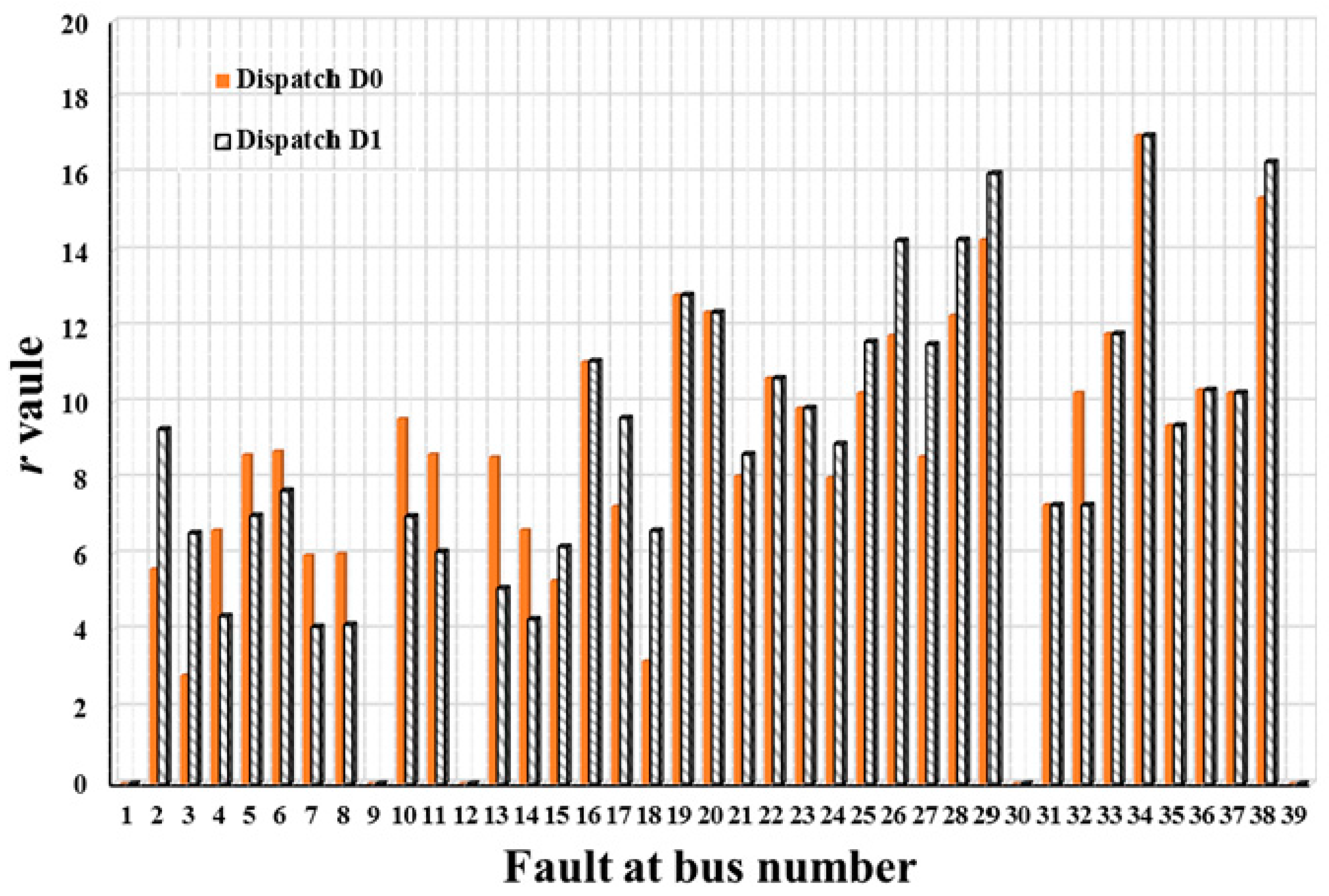
4.3.2. Comparison between Dispatch D₀ and D₁

The details of implementations and calculations of the stability index modules for the fault at bus 2 in dispatch D₀ were explained in the previous section. In this section, a comparison of the stability indices for dispatches D₀ and D₁ as an example is provided. Local stability index r values for other fault locations (buses) for dispatch D₀ are presented in Figure 4, along with similar values for dispatch D₁. Considering the overall performance of a system for a given dispatch, the proposed composite global index R, which is the summation of r values for all tested buses, provides an overview of transient stability performance. The composite R value, summation of all r values shown in Figure 4, yields R = 315.404 for D₀, and R = 319.937 for D₁. A larger R value indicates a worse transient stability performance. Thus, in the given example, D₁ is worse than D₀ in terms of transient stability performance. This does not necessary mean that all the local stability for D₁ is worse than D₀, and that a comparison of the local stability r values should also be conducted.

In Figure 4, the solid filled bars represent r values for dispatch D₀ and the pattern-filled bars represent r values for dispatch D₁. The r values for both dispatches at every bus of the system are compared side by side. The r values for D₀ and D₁ can be categorized into three groups, as given below. Each group corresponds to certain number of buses shown by red, green, and black colors in Figure 5. To clarify, these buses are:

Group 1

black buses: 1, 9, 12, 19, 20, 22, 30, 31, 33, 34, 35, 36, 37 and 39.

Group 2

green buses: 4, 5, 6, 7, 8, 10, 11, 13, 14 and 32.

Group 3

red buses: 2, 3, 15, 16, 17, 18, 21, 23, 24, 25, 26, 27, 28, 29 and 38.

Group 1 represents those buses that have r values with no changes or very small changes (less than a tolerance of 0.01) between D₀ and D₁. For some buses, such as 1, 9, 12, 30 and 39, the values were 0. At other buses, such as 19, 20, 22, 31, 33, 34, 35, 36 and 37, the values remained essentially the same. Group 2 represents those buses for which the r values for D₁ dispatch are lower than those in D₀. Group 3 represents those buses for which the r values for D₁ dispatch are higher than those in D₀. For example, in Group 3, bus 16 represents a very small increase in local stability r value, as shown in Figure 5. This small increase is from the changes in Vsag module between D₀ (dash curves) and D₁ (solid curves), as shown in Figure 6. The worst voltage sags occur at 0.774, 0.719 and 0.625 pu (marked as black square data-tip on dash lines) at FCTs 8-, 9-, and 10- cycle, respectively, for dispatch D₀. Thus, the Vsag module f₄ results are 0.226, 0.281, 0.375, respectively, as shown in

Table 3. Comparison of r_Bus16 value between dispatch D₀ and D₁.

Fault Location	Clearing Time (Cycles)	Dispatch D0				Dispatch D1
		SS (f1)	LOS (f2)	Damping (f3)	Vsag (f4)	SS (f1)	LOS (f2)	Damping (f3)	Vsag (f4)
Bus2	1	0	0	0	0	0	0	0	0
Bus2	2	0	0	0	0	0	0	0	0
Bus2	3	0	0	0	0	0	0	0	0
Bus2	4	0	0	0	0	0	0	0	0
Bus2	5	0	0	0	0	0	0	0	0
Bus2	6	0	0	0	0	0	0	0	0
Bus2	7	0	0	0	0	0	0	0	0
Bus2	8	0	0	0	0.226	0	0	0	0.231
Bus2	9	0	0	0	0.281	0	0	0	0.290
Bus2	10	0	0	0	0.375	0	0	0	0.402
Bus2	11	1	N/A	N/A	N/A	1	N/A	N/A	N/A
Bus2	12	1	N/A	N/A	N/A	1	N/A	N/A	N/A
Bus2	13	1	N/A	N/A	N/A	1	N/A	N/A	N/A
Bus2	14	1	N/A	N/A	N/A	1	N/A	N/A	N/A
Bus2	15	1	N/A	N/A	N/A	1	N/A	N/A	N/A
Bus2	16	1	N/A	N/A	N/A	1	N/A	N/A	N/A
Bus2	17	1	N/A	N/A	N/A	1	N/A	N/A	N/A
Bus2	18	1	N/A	N/A	N/A	1	N/A	N/A	N/A
Bus2	19	1	N/A	N/A	N/A	1	N/A	N/A	N/A
Bus2	20	1	N/A	N/A	N/A	1	N/A	N/A	N/A
		rBus16 = 10.882				rBus16 = 10.923

. Similarly, the Vsag module f₄ results are 0.231, 0.290, 0.402, respectively, for dispatch D₁. FCTs from 11 cycles to 20 cycles at bus 16 cause system separation for Dispatch D₀ and D₁. Therefore, the r_Bus16 values, the summation of f₁, f₂, f₃, and f₄ values, are found to be 10.882 for D₀ and 10.923 for D₁. The increase is 0.041.

As another example, Group 3 is discussed. Group 3 undergoes a bigger r value increase. The r values at bus 2 (r_Bus2) for the D₀ and D₁ are 5.61 and 9.3, respectively, as shown in Figure 4. This is mainly because the system separation occurs earlier for D₁ than D₀. In summary, the r values for the buses in Group 3 are higher for D₁, compared to D₀, because G9’s real power increases by 100 MW, thus moving G9 closer to its angular stability limit. Conversely, the r values for the buses in Group 2 are smaller for D₁ compared to D₀, because G3’s real power decreases by 100 MW, moving G3 further away from its stability limit. The local stability index r values are certainly affected by the dispatch changes. The r value is thus considered the local stability performance index at a specific location, for a particular system configuration. Using the r values for grouping buses can provide a useful way to quantify and visualize the effect of system configuration changes on the transient stability performance.

4.3.3. Normalized Index Presentation

The analysis results can be presented using an alternate, normalized performance index, which reflects the violation occurrence frequency for each system configuration. The normalized R_n index (instability likelihood) is defined as:

$${\mathit{R}}_{\mathit{n}}=\frac{\mathit{R}}{N}$$

(14)

where R_n is normalized value of stability index R over the number of simulations N for one dispatch. In this case, N equals 780 (20 simulations for 39 buses in the system).

Table 4. Stability index over 780 simulations for each dispatch,

Index	D0	D1	D2	D3	D4	D5
R	315.404	319.937	308.417	295.182	477.585	780
Rn	40.44%	41.02%	39.54%	37.84%	61.23%	100%

summarizes the stability index R and R_n for all tested dispatches with TSPQ method.

Table 4 shows that D₅ has the highest R and R_n value. Therefore, this dispatch is the least reliable and system operators should avoid it. In the planning stage, this dispatch requires the most attention. The next least reliable dispatch is D₄. D₃ is the most reliable dispatch compared to others, because D₃ has the lowest R value. R gives power system planners a very good sense of the severity of each contingency and of the system strength. It should be noted that dispatch D₅, where all the generators operate at maximum power, exhibits system separation for all the applied contingencies. This clearly unreasonable configuration is included to illustrate the module-ranking logic adopted in this study: the SS (f₁) module value is 1 for all contingencies in this case. While the R value provides an overall stability performance measure, the differences in R values need to be scrutinized in terms of local stability index in each module, as discussed in the above sections. The proposed analysis method could certainly be expanded to include modules corresponding to additional assessment criteria.

5. Implementation on a Real Power System

To illustrate the result of the TSPQ methodology on a real system, the Northeast Interconnection Power System (NIPS) model was used. The system has a total of 65844 buses, 8703 generators (6968 plants), 35425 loads, 84694 branches, and 40 DC lines. The focus is on a region of NIPS, the ISO New England transmission system, which has 737 generators (553 plants), 1459 loads, 2984 branches, and 3 DC lines.

Contingencies and Dispatches: Although the TSPQ analysis method will always offer outstanding post-processing time gains, the simulations volume—i.e., base case, dispatches and contingencies selection—is normally determined through engineers’ collective judgment of the project’s objectives. Three summer light load (SLL) dispatches SLL₁, SLL₂, and SLL₃, and one summer peak (SP) case SP₁ were chosen for this study. The SLL₁, SLL₂, and SLL₃ dispatches represent a New England load of 12,500 MW, and SP₁ represents a New England load of 31,500 MW. All four cases used the same steady state and dynamic models. While SLL₁, SLL₂, and SLL₃ have the same load, the difference between them is in their power transfer levels at different flowgates (power transfer corridors) to stress major regions of the transmission system. SLL₁ and SLL₂’s transfer levels were stressed at different flowgates in Maine, and SLL₃’s transfer levels were stressed at flowgates outside of Maine.

The contingencies selection was limited to Maine locations since the objective was only to test the TSPQ methodology. Furthermore, to reduce the data volume, the following two-step automated screening process was applied before applying the TSPQ methodology:

(1)

A total of 108 assumptive, three-phase fault contingencies with a pessimistic 10 s clearing time was applied at stations with voltages equal and above 115 kV across Maine as shown in the New England Geographic Transmission Map [22]. If any of these contingencies did not cause a criteria violation based on [11,14,15,16,17], it was removed from further consideration, to limit the data volume to only the non-trivial faults.

(2)

The locations where the 10 s duration three-phase contingency resulted in stability violations were re-tested by applying three-phase faults with the actual, normal clearing times (4–6 cycles range). The simulation results files were then analyzed through the TSPQ methodology and the findings are included in this report.

TSPQ Method Results: The TSPQ method, as explained above, was applied to the simulation results of the locations that failed the 10s clearing faults but were re-tested with the actual fault clearing times as provided by utilities. The details of stability criteria values used in the TSPQ modules were taken from an ISO New England report [11]. According to these criteria, $P_{Limi{t}_C}$ in Equation (3) is defined as 1400 MW and the damping ratio and voltage sag criteria remain the same, as given in Equations (5), and (7)–(9).

Figure 7, Figure 8, Figure 9 and Figure 10 illustrate 256 representative angle and voltage performance of buses in the ISO New England region for a particular contingency, with the actual clearing time. Figure 7 and Figure 8 show the rotor angles of the most significant generators (not less than 2 MW) in New England. They also show the bus voltages, 115 kV level and above, during and after the particular fault for dispatch SLL₁. All buses across New England were monitored and examined through the comprehensive TSPQ method. The plots confirm the results reported by the TSPQ analytical method: there are no system separations and no voltage sags or damping violations after the faults were cleared. The total loss of source is less than 1400 MW (see Figure 7 for tripped generators), thus the r values for this contingency is zero at all the locations.

Figure 9 and Figure 10 show the same contingency and same buses in Figure 7 and Figure 8, but this time for dispatch SLL₂. For this case, the figures show system separation, a total loss of source of more than 1400 MW, and voltage sags. However, system separation has higher priority and remaining modules are not called (see Equation (13)); thus, the r value for the same contingency but a different dispatch is now 1, for all the locations.

Similarly, the r value for each of the 49 Maine contingencies (bus fault locations) for dispatches SLL₁, SLL₂, SLL₃ and SP₁ were calculated by using Equation (12). The Index R for these dispatches are shown in

Table 5. Stability index over 49 contingencies in maine.

Index	SLL1	SLL2	SLL3	SP1
R	22	26	21	21
Rn	44.9%	53.06%	42.86%	42.86%

. A comparison of the R values shows that SLL₂ with R = 26 presents the worst dispatch scenario. A comparison of dispatches SLL₁ and SLL₂ is shown in Figure 11. For dispatch SLL₁, there are 22 blue color buses that demonstrate system separation (local stability equals 1). For dispatch SLL₂, an additional four red-color buses experience system separation. The global stability index R provides a quick quantification and ranking value. The detailed analysis for each module is available if needed. Note that the stability indices r and R are effective screening tools, intended to uncover and rank violations, but not as a substitute for thorough engineering analysis.

6. Conclusions

This paper discusses a systematic and comprehensive transient stability performance quantification (TSPQ) methodology for power system assessment. System separation, loss of source, damping analysis, and voltage sag assessment modules were considered in the TSPQ method discussed in this paper. It was suggested that the methodology is expandable to include other modules where applicable. It was shown, through the application of the methodology to an IEEE 39-bus system and the current ISO New England transmission system, how the use of the global stability index R (the summation of local stability index r values) quantifies the transient performance of a system subjected to given disturbances. The TSPQ method was shown to be an efficient and comprehensive data mining tool that can quantify the effect of different dispatches and contingencies on the transient stability of power systems. It was suggested that, by providing the ability to sort the violations by severity, the TSPQ method can help identify potential mitigation solutions to specific locations and operating conditions.

References

1. Northeast Power Coordinating Council, Inc. Classification of Bulk Power System Elements, Document A-10; NPCC Inc.: New York, NY, USA, 2009. [Google Scholar]
2. North American Electric Reliability Corporation. Standard TPL-001-4—Transmission System Planning Performance Requirements; NERC: Atlanta, GA, USA, 2016. [Google Scholar]
3. Zhu, Y.; Brown, D. Enhancing stability simulation for NERC Reliability Standard TPL-001-4 compliance. In Proceedings of the EPEC, London, ON, Canada, 26–28 October 2015. [Google Scholar]
4. Fouad, A.A.; Kruempel, K.C.; Vittal, V.; Ghafurian, A.; Nodehi, K.; Mitsche, J.V. Transient Stability Program Output Analysis. IEEE Trans. Power Syst. 1986, 1, 2–8. [Google Scholar] [CrossRef]
5. Maria, G.A.; Tang, C.; Kim, J. Hybrid Transient Stability Analysis [Power System]. IEEE Trans. Power Syst. 1990, 5, 384–393. [Google Scholar] [CrossRef]
6. Tang, C.K.; Graham, C.E.; El-Kady, M.; Alden, R.T.H. Transient Stability Index from Conventional Time Domain Simulation. IEEE Trans. Power Syst. 1994, 9, 1524–1530. [Google Scholar] [CrossRef]
7. Ma, F.; Luo, X.; Litvinov, E. Cloud Computing for Power System Simulations at ISO New England—Experiences and Challenges. IEEE Trans. Smart Grid 2016, 7, 2596–2603. [Google Scholar] [CrossRef]
8. Smith, S.; Woodward, C.; Min, L.; Jing, C.; Rosso, A.D. On-line transient stability analysis using high performance computing. In Proceedings of the 2014 IEEE PES Innovative Smart Grid Technologies Conference (ISGT), Washington, DC, USA, 19–22 February 2014. [Google Scholar]
9. Meng, K.; Dong, Z.Y.; Wong, K.P. Enhancing the computing efficiency of power system dynamic analysis with PSS_E. In Proceedings of the IEEE International Conference on Systems, Man and Cybernetics, San Antonio, TX, USA, 11–14 October 2009. [Google Scholar]
10. Chen, S.; Onwuachumba, A.; Musavi, M.; Lerley, P. Transient Stability Performance Quantification Method for Power System Applications. In Proceedings of the Power Systems Conference (PSC), Clemson, SC, USA, 8–11 March 2016. [Google Scholar]
11. ISO New England Inc. Transmission Planning Technical Guide Appendix F; ISO New England: Holyoke, MA, USA, 2013. [Google Scholar]
12. Fouad, A.A.; Vittal, V. Power System Response to a Large Disturbance: Energy Associated with System Separation. IEEE Trans. Power Appar. Syst. 1983, 102, 3534–3540. [Google Scholar] [CrossRef]
13. IEEE/CIGRE Joint Task Force on Stability Terms and Definitions. Definition and Classification of Power System Stability. IEEE Trans. Power Syst. 2004, 19, 1387–1401. [Google Scholar]
14. Siemens Power Technologies International. Stability Study Report for Q371 Wind Project Interconnecting to Line L-163 near Jackman 115 kV Substation in New Hampshire Prepared for ISO-NE, 30 November 2012. Available online: https://www.nhsec.nh.gov/projects/2015-02/application/documents/10-02-15-sec-2015-02-appendix-6-final-redacted-non-ceii-r110-11-final-stability-study-rpt-fo.pdf (accessed on 5 July 2017).
15. ISO New England Stability Task Force. Damping Criterion Basic Document; ISO New England: Holyoke, MA, USA, 2009. [Google Scholar]
16. Reliability Standards for the New England Power Pool; NEPOOL Planning. Procedure NO. 3; ISO-NE: Holyoke, MA, USA, 2004.
17. ISO New England Inc. Transmission Planning Technical Guide Appendix E, Dynamic Stability Simulation Voltage Sag Guideline; System Planning; ISO New England Inc.: Holyoke, MA, USA, 2013. [Google Scholar]
18. ISO New England Inc. ISO New England Planning Procedure No. 5–6, Interconnection Planning Procedure for Generation and Elective Transmission Upgrades; ISO New England: Holyoke, MA, USA, 2016. [Google Scholar]
19. ISO New England Inc. Transmission Planning Technical Guide, 15 January 2016. Available online: https://www.iso-ne.com/static-assets/documents/2016/01/planning_technical_guide_1_15_16.pdf (accessed on 5 July 2017).
20. Pai, M.A. Energy Function Analysis for Power System Stability; Springer: New York, NY, USA, 1989. [Google Scholar]
21. Athay, T.; Podmore, R.; Virmani, S. A Practical Method for the Direct Analysis of Transient Stability. IEEE Trans. Power Appar. Syst. 1979, 98, 573–584. [Google Scholar] [CrossRef]
22. ISO New England Inc. New England Geographic Transmission Map through 2024, 2014. Available online: https://www.iso-ne.com/static-assets/documents/2015/05/2015_celt_appendix_f.pdf (accessed on 4 February 2017).
Figure 1. Proposed transient stability analysis procedure.
Energies 10 00984 g001
Figure 2. Voltage sags at buses 26, 28, and 29.
Energies 10 00984 g002
Figure 3. System separation between G9 and others.
Energies 10 00984 g003
Figure 4. Comparison of local stability indices for dispatches D0 and D1.
Energies 10 00984 g004
Figure 5. r value changes on dispatch D1.
Energies 10 00984 g005
Figure 6. Voltage sags changes at bus 16.
Energies 10 00984 g006
Figure 7. No system separation for dispatch SLL1.
Energies 10 00984 g007
Figure 8. No voltage sags for dispatch SLL1.
Energies 10 00984 g008
Figure 9. System separation for dispatch SLL2.
Energies 10 00984 g009
Figure 10. Voltage sags for dispatch SLL2.
Energies 10 00984 g010
Figure 11. One-line diagram comparison for dispatches SLL1 and SLL2.
Energies 10 00984 g011