Article

An Improved Ångström-Type Model for Estimating Solar Radiation over the Tibetan Plateau

1
State Key Laboratory of Severe Weather, Chinese Academy of Meteorological Sciences, Beijing 100081, China
2
Regional Climate Group, Department of Earth Sciences, University of Gothenburg, SE-405 30 Gothenburg, Sweden
3
Key Laboratory of Land Surface Pattern and Simulation, Institute of Geographic Sciences and Natural Resources Research, Chinese Academy of Sciences, Beijing 100101, China
4
Center for System Integration and Sustainability, Michigan State University, East Lansing, MI 48823, USA
5
Plant Functional and Climate Change Cluster, University of Technology, Sydney 2007, Australia
6
USDA-ARS, Northwest Watershed Research Center, Boise, ID 83712, USA
7
NSW Department of Primary Industries, Wagga Wagga Agricultural Institute, PMB, Wagga Wagga, NSW 2650, Australia
8
University of Chinese Academy of Sciences, Beijing 100049, China
9
Climate Center, Tibet Autonomous Meteorological Administration, Lhasa 850000, China
10
Centre for Solar and Wind Energy Research, China Meteorological Administration, Beijing 100081, China
*
Author to whom correspondence should be addressed.
Energies 2017, 10(7), 892; https://doi.org/10.3390/en10070892
Submission received: 3 May 2017 / Revised: 14 June 2017 / Accepted: 23 June 2017 / Published: 1 July 2017

Abstract

:
For estimating the annual mean of daily solar irradiation in plateau mountainous regions, observed data from 15 radiation stations were used to validate different empirical estimation methods over the Tibetan Plateau. Calibration indicates that sunshine-based site-dependent models perform better than temperature-based ones. Then, the highly rated sunshine-based Ångström model and temperature-based Bristow model were selected for regional application. The geographical models perform much better than the average models, but still not ideally. To achieve better performance, the Ångström-type model was improved using altitude and water vapor pressure as the leading factors. The improved model can accurately predict the coefficients at all the stations, and performs the best among all models with an average Nash-Sutcliffe Efficiency value of 0.856. Spatial distribution of the annual mean of daily solar irradiation was then estimated with the improved model. It is indicated that there is an increasing trend of radiation from east to west, with a great center of the annual mean of daily solar irradiation on southwest Tibetan Plateau ranging from 20 to 24 MJ·m−2. The improved model should be further validated against observations before its applications in other plateau mountainous regions.

1. Introduction

Solar radiation plays a critical role in most land surface processes including physical, biological and chemical processes, e.g., hydrological cycling, vegetation growth, climate and weather change [1,2,3,4]. It is also one of the key input variables in crop growth, and hydrological and climate models [5,6,7,8,9]. However, unlike other meteorological elements such as temperature and precipitation, solar radiation is observed only at very few stations due to scarcity of instruments and high cost of maintenance [5,10]. Thus, estimation of solar radiation becomes an indispensable method for energy harvest and model application.
Several methods are available for solar radiation estimation including numerical models, artificial neutral networks, satellites measurements, etc. Some complex dynamic numerical models were established based on meteorological theory for the relationships between solar radiation and other meteorological variables, including aerosol concentrations [11,12]. This kind of model usually requires many input variables that can hardly be applied practically. Solar radiation can also be estimated by artificial neutral network [13,14,15,16,17] and satellite-based remote sensing methods [18,19,20]. However, training neutral network usually requires large datasets and the resulting model may not be applicable to other regions [10]. The low sampling frequency resulting from cloudiness and the coarse spatial resolution always make satellite-based remote sensing methods inadequate for site-specific application [21]. In addition, there is no satellite-based database covering the Tibetan Plateau (TP) except the National Aeronautics and Space Administration-Surface meteorology and Solar Energy (NASA-SSE) product and several commercially-available products by companies. The NASA-SSE is free, but is currently limited to 1983 to 2005 [22]. In contrast to the models mentioned above, several simple empirical models have been developed and widely used as the primary tools for solar radiation estimation. These are typically based on the relationship between solar radiation and readily available meteorological variables, such as sunshine hours [23,24,25,26,27], temperature [28,29,30,31,32,33], and precipitation [34,35]. Many previous studies have established that the sunshine-based models always outperform other types of models [30,36,37,38,39].
Requirements of empirical models are relatively easy to meet, and the models themselves are easy to apply. However, the necessity to calibrate empirical models indicates that their coefficients are changing with locations, e.g., [9,30,34,37,40,41,42]. The site-dependent coefficients restrict regional application of the empirical models, which is a big challenge for spatial rasterization. To solve this problem, the model coefficients for regional application were obtained by simply averaging coefficients at different locations [43], or fitting coefficients from an overall regional database combining all of the datasets at different locations [44]. In the view of statistical theory [45], both of these two methods have the same premise that the variation in coefficients should be small between different locations, which seems to be supported by previous reports made in the plain regions [42,44]. However, up to now, this assumption has never been tested thoroughly under complex terrain conditions. Recently, some geographic models were also developed for regional applications [46,47,48,49,50] by means of fitting the coefficients with geographical information such as latitude, longitude and altitude. Although these models perform quite well in the plain regions, they have not been tested thoroughly under complex terrain conditions like the TP. Thus, integrated comparison and evaluation of different ways of determining regional coefficients of the empirical models are needed for future applications in the complex terrains conditions, like the Tibetan Plateau.
Located in Southwest China and known as the Third Pole, the TP is the highest contiguous region in the world, and has abundant solar energy resources because of its high elevation [51]. However, up to now, few research studies on solar radiation estimation over the TP have been made, compared to the numerous reports on the plain regions, e.g., [30,34,36,37,42]. Pan et al. [52] proposed a method to rasterize daily global solar radiation over the TP based on the diurnal temperature ranges with the Bristow-Campbell model, but the Bristow-Campbell model is a temperature-based model, which is thought to be inferior to the sunshine-based ones [30,36,37,38,39]. Li et al. [53] evaluated the performance of eight sunshine-based models on the TP, and proposed two average models for estimating solar radiation on the TP, based on fitting coefficients to the composite database involving all selected stations. However, the coefficients of the sunshine-based models reflect the transmission characteristics of the atmosphere at its calibration site [42], which is determined by the optical path of the sunlight affected by the altitude [54], we can reasonably hypothesize that coefficients of the sunshine-based models would vary greatly due to great variation of the altitude under complex terrain conditions, meaning that the models suggested by Li et al. [53] can only be used to estimate solar radiation at certain locations on the TP. Thus, an innovative sunshine-based model has to be developed for more accurate estimation of the distribution of solar radiation under complex terrain conditions on the TP.
In this study, the annual mean of daily solar irradiation from 15 solar stations on the TP and its surrounding regions were collected and analyzed. The objectives of this research are: (1) to thoroughly test the hypothesis that the coefficients of the empirical models vary considerably on the TP and its adjacent areas; (2) to compare the performances of different methods on determining regional coefficients of the empirical models over the TP; and (3) to identify the leading factors accounting for the variations in coefficients and develop an innovative simple sunshine-type model for accurate estimation of the distribution of the annual mean of solar irradiation over the TP.

2. Results

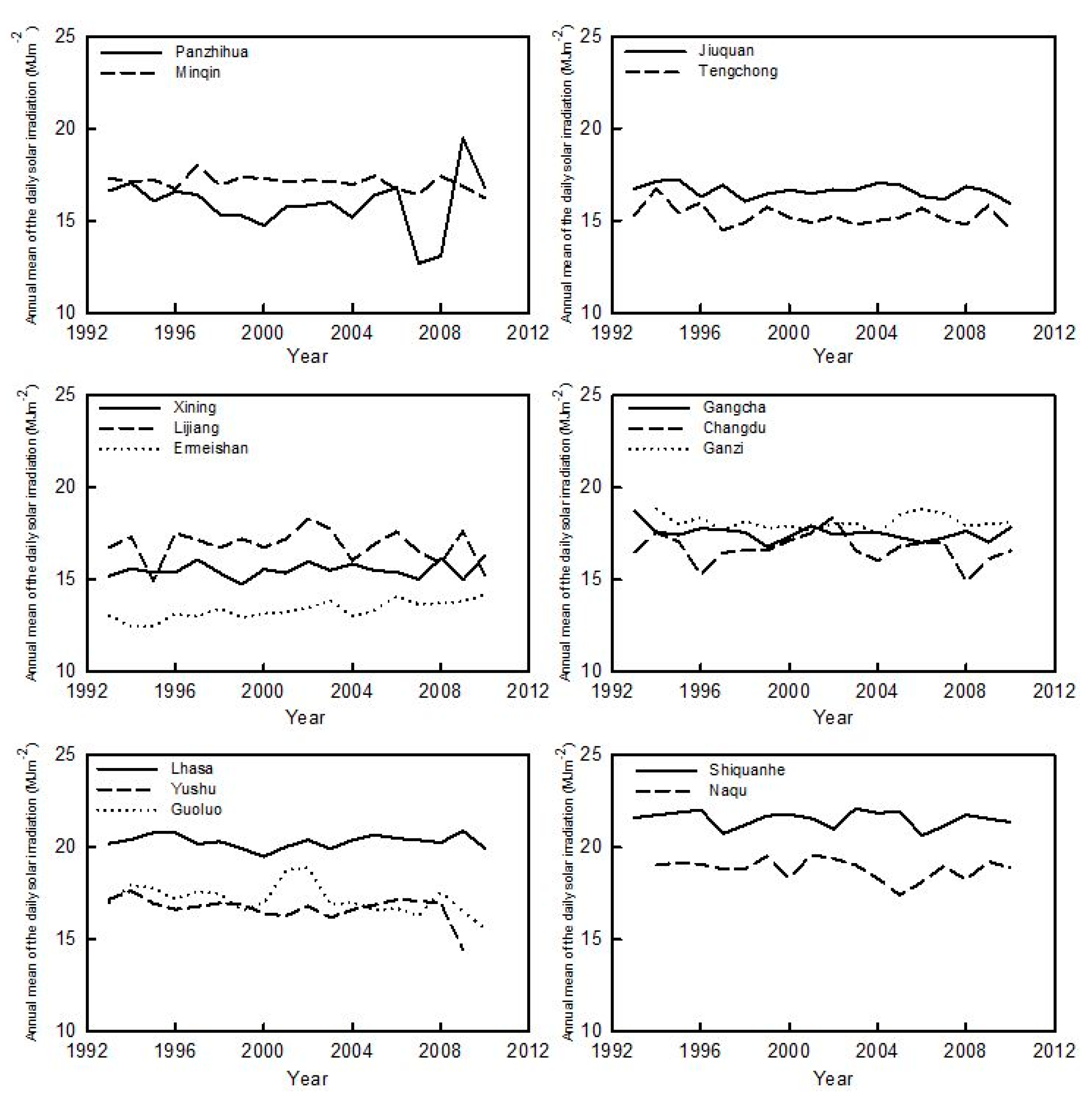
2.1. Spatial and Temporal Pattern of Observed Annual Mean of Solar Irradiation

The fifteen radiation stations were classified into six groups according to altitude, and the variations of the annual mean of daily solar irradiation from 1993 to 2010 for each group can be seen in Figure 1. Generally speaking, temporal variations are relatively stable at all stations except an abrupt drop around 2008 at Panzhihua. There is a general trend that the annual mean of daily solar irradiation becomes greater with increasing altitude. The annual mean of daily solar irradiation on the TP, such as at Lhasa, Shiquanhe and Naqu, is much greater than that in its surrounding regions like Panzhihua. The lowest annual mean of daily solar irradiation occurs in Ermeishan with a value of 13.35 MJ·m−2, due to large cloud coverage. The greatest annual mean of solar irradiation occurs at Shiquanhe, with a value of 21.49 MJ·m−2. Greater annual mean of daily irradiation on the TP again validates the assumption that abundant solar energy resources are held on the TP due to its higher elevation [38,51]. These data are fundamental supports for the validation of estimated spatial radiation distribution on the TP.

2.2. Comparison of the Performances of Different Methods on Estimation of Daily Solar Irradiation

The coefficients of site-dependent models were first fitted for each of the selected 15 stations. Each pair of the coefficients of a and b relates to the corresponding station, meaning that these coefficients cannot be used in the regional scale. However, based on these coefficients, regional coefficients are obtained by average, geographical, and modeling methods as follows.

2.2.1. Site-Dependent Models

First, the three sunshine-based models, Ångström, Ogelman and Bahell, were calibrated with the datasets from 1993 to 2007 (Table 1). Coefficients of a and b in the Ångström model range from 0.173 in Panzhihua to 0.291 in Ganzi, and from 0.498 in Panzhihua to 0.603 in Changdu, respectively. Similar variations can also be found in the coefficients of Ogelman and Bahell models. Though the coefficients are different for different stations, the average values of NSE of the three sunshine-based models are nearly the same, with values of 0.885, 0.886 and 0.887 respectively. The other evaluation indicators such as MAPE, RRMSE, Slope and Inter also confirm the similar model performance. The three temperature-based models were then calibrated at each station using the same period of data (Table 1). The coefficients of a, b and c in Bristow model also vary considerably, ranging from 0.601 in Panzhihua to 1.005 in Changdu, from 0.005 in Gangcha to 0.057 in Tengchong, and from 1.18 in Tengchong to 2.340 in Gangcha, respectively. Similar variations in the coefficients can also be found in the calibration results of the Hargreaves and Chen models. The NSE values of the three temperature-based models are also quite similar, with average values of 0.672, 0.671 and 0.673, respectively. Compared with the sunshine-based models, the NSE values of the three temperature-based models are much lower, indicating sunshine-based models have obvious advantages over the temperature-based ones in model calibration on the TP.
The calibrated coefficients of the site-dependent models were then used to predict daily solar irradiation at different stations, and the model performance is shown in Table 2. Comparison between Table 1 and Table 2 indicates that model prediction performed a little worse for the validation period compared to the calibration period for both sunshine- and temperature-based models, which is a normal phenomenon in the view of statistical theory [45]. However, changes in NSE and the other evaluation indicators within and between the sunshine- and temperature-based models are quite similar to those for the calibration period. Differences in model performance were further analyzed by t-test (Figure 2), and the results indicate lower t values exist within the results from sunshine- or temperature-based models, but the t value is greater between the results from sunshine- and temperature-based models (though not significant with t0.05 test), showing great difference exists between the performance of the sunshine- and temperature-based models.
On the whole, the sunshine-based models performed better than the temperature-based ones, but only small differences in model performance exit within sunshine- or temperature-based models themselves. So the highly rated Ångström and Bristow models, representing the sunshine- and temperature-based model respectively, were selected for further study on developing average and geographical models in the following sections.

2.2.2. Average Models

Regional coefficients of a and b in the Ångström model were obtained by simply averaging the coefficients calibrated at the fifteen radiation stations, then daily solar irradiation was predicted at each station by the same coefficients of a and b, with values of 0.229 and 0.549 respectively. As mentioned above, the coefficients of a and b vary greatly between different stations, thus using the average coefficients to represent all of the coefficients at the fifteen stations will cause bigger error than the models with site-dependent coefficients. Comparison of Table 2 and Table 3 shows the difference in model performance at all the stations for the Ångström model. The average NSE of the simple average mode is 0.826, also lower than the corresponding value of 0.865 in the site-dependent model. The two smallest values of NSE validated by the site-dependent model is 0.700 in Panzhihua and 0.781 in Tengchong, while the two smallest values of NSE validated by the simple average model are only 0.586 in Tengchong and 0.596 in Panzhihua, respectively. Performance of the Bristow-type simple average model is also shown in Table 3. No values of the NSE were lower than 0.400 in the performance of the site-dependent Bristow model (Table 2), whereas there are 5 out of 15 stations with NSE values lower than 0.400 for the Bristow-type simple average model (Table 3).
Performance of the statistical average model can also be seen in Table 3. The coefficients of a and b in the Ångström-type statistical model are 0.229 and 0.550 respectively, nearly the same as those in the corresponding simple average model. Estimation of daily solar irradiation at 15 stations with the nearly same coefficients leads to a very similar model performance between Ångström-type simple average model and the corresponding statistical average model (Table 3). In contrast, the coefficients of the Bristow-type statistical average model are quite different from those of the Bristow-type simple average model. All in all, the Bristow-type statistical average model performed better than the Bristow-type simple average model at 11 out of 15 stations based on NSE (Table 3).
In short, the Ångström-type simple average model performs nearly the same as the Ångström-type statistical average model, and both of the models are better than the Bristow-type simple/statistical average models. Among all of the average models, the Bristow-type simple average model performed the worst, even having a negative NSE value at Changdu station.

2.2.3. Geographical Models

Coefficients of the site-dependent Ångström/Bristow models at 15 stations (Table 1) were fitted with their corresponding geographical parameters, and the multiple linear models linking the coefficients and the geographical parameters were shown in Table 4.
The geographical models are somewhat more complex than the simple/statistical average models with more geographical parameters involved. Thus, the geographic model would be expected to perform better than the simple/statistical average models. However, Ångström-type geographical model performs almost the same as the corresponding average models, while the Bristow-type geographical model performed better than the corresponding simple average model but worse than the statistic one (Table 5). In addition, the better performed Ångström-type geographical model cannot be applicable under extreme conditions, e.g., in the mountain Everest with altitude 8844.43 m, due to its unacceptable coefficient (a + b) greater than 1. This will be further discussed in the below sections.

2.2.4. Improved Ångström-Type Model

As mentioned above, the sunshine-based Ångström model is superior to the temperature-based Bristow model. Therefore, the Ångström model was selected to develop a new model for regional application on the TP and its surrounding regions. For development of the regional model, suitable equations should be established to account for the variations in the coefficients of Ångström model on the TP and its surrounding regions. Therefore, variations in the coefficients of Ångström model was analyzed first. Coefficients of a, b and (a + b) at 15 radiation stations are given in Figure 3, indicating not only a and b but also the sum of (a + b) vary greatly on the TP and its surrounding regions.
To account for the great variation in the coefficients in Figure 3, more than one hundred of different mathematical functions and variable combinations were tested to find the best equation to fit the relationship between coefficients of Ångström model and the related geographical or meteorological factors. The leading factor accounting for the variation in coefficient b was identified as water vapor pressure, and a reciprocal relation was established between the coefficient b and the corresponding averaged daily water vapor pressure (Figure 4a). We failed to find the suitable equation for fitting the coefficient a, though it is believed that coefficient a is related to cloudiness [42]. However, it was found that the sum of coefficients (a + b) correlated well to the altitude as a logarithm function (Figure 4b). Thus, the improved Ångström-type model can be expressed as follows:
H H 0 = a + b S S 0
If S = S0, i.e., cloud-free conditions, then H = (a + b)H0. Since the clearness index Kt is defined as H = KtH0, (a + b) = Kt in the cloud-free conditions. When S = 0, i.e., overcast conditions, then H = aH0, and a is equal to Kt in overcast conditions.
a + b = 0.106 × ln ( A l t ) 0.060
b = 0.373 × 1 V a p + 0.483
where A l t is altitude (m), and V a p is the average daily water vapor pressure (hPa). Linear regressions between coefficients and leading factors indicate that the improved model accounts fairly well for variations in the coefficients of the Ångström model (Figure 4).
Validation of the improved Ångström-type model indicates that it performs better than the average and geographical models (Table 6). In addition, the improved Ångström-type model can also account for the variations in coefficients better than the average and geographical models. Performance of the different kinds of models in predicting annual mean of daily solar irradiation at Lhasa in the validation period 2008–2010 is shown in Figure 5, indicating vividly that improved Ångström-type model performs much better than the average and geographical models. Note that it is only fortuitous that the NSE of the geographical model is even greater than those of the site-dependent Ångström, Ogelman and Bahell models. The NSE values of the improved Ångström-type model are generally slightly lower than those of the site-dependent models (Table 2 and Table 6). Figures drawn for the other stations are quite similar to Figure 5, and were not shown due to the limitation of space.
As mentioned above, the improved Ångström-type model performs much better than the average and geographical models, with higher skill in accounting for the coefficient variations. Thus, the improved Ångström-type model was selected to estimate the spatial distribution of the annual mean of daily solar irradiation on the TP.

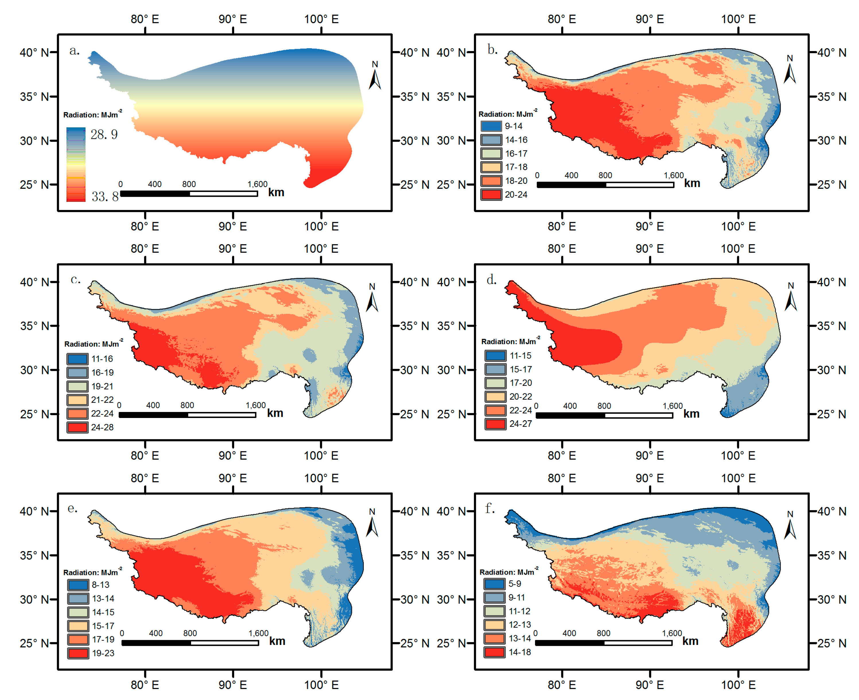
2.3. Estimation of the Spatial Distribution of the Annual Mean of Daily Solar Irradiation with the Improved Ångström-Type Model

The spatial distribution of the annual mean of daily solar irradiation was estimated by the improved Ångström-type model using gridded 1 km × 1 km sunshine percentage and water vapor pressure interpolated over the region. The first step was to validate the ANUSPLIN interpolation method on the TP. To do so, water vapor pressure data measured at 8 stations in the period 1993–2010 were selected as a validation dataset. Then, water vapor pressure from the other weather stations was used as input to the ANUSPLIN software to interpolate the gridded water vapor pressure data over the TP. The interpolated water vapor pressure at the 8 selected stations in the period 1993–2010 were used to validate against the measured ones, and the result of the validation indicated that a reliable and accurate interpolation could be done by ANUSPLIN interpolation method (Figure 6a). Validation of the sunshine percentage showed similar result as that for water vapor pressure (Figure 6b).
Based on these results, the spatial distribution of water vapor pressure and sunshine percentage on the TP was interpolated (Figure 7b,c), based on which the coefficients of (a + b), b and a were rasterized by the improved Ångström-type model using the ArcGIS 10.3 platform (Figure 7e,f).
Extra-terrestrial radiation is defined as the solar radiation received at the top of the earth’s atmosphere on a horizontal surface, and is only a function of latitude, date and length of the daytime. By accumulation of the time, the annual daily extra-terrestrial radiation should be distributed latitudinally. The extra-terrestrial radiation calculated according to Allen et al. [9] exactly fits this basic common knowledge (Figure 8a). Finally, the coefficients of a and b, sunshine percentage and the extra-terrestrial radiation were used as input variables to drive the improved Ångström-type model for estimation of the annual mean of daily solar irradiation on the TP. Both annual and seasonal spatial distribution of the annual mean of daily solar irradiation were rasterized in Figure 8b–f. Generally speaking, the annual mean of daily solar irradiation is greater in spring and summer and less in the autumn, and radiation increases from east to the west, with greatest values in the southwest part of the TP. The notable exception of the greatest annual mean of daily solar irradiation located in the most south TP for the winter in Figure 8f might be attributed to grater coefficients b aroused by the lower water vapor pressure and greater extra-terrestrial radiation in this region in winter days. Annual mean of daily solar irradiation has a similar spatial distribution to those of the seasonal, ranging from 9 MJ·m−2 in the east to the 24 MJ·m−2 in the southwest TP.

3. Discussion

The main objective of this research is to develop a suitable method for estimating the annual mean of daily solar irradiation under complex terrain conditions like the TP. Based on the annual mean of daily solar irradiation measured over the TP and its surrounding regions, we have identified the variation of coefficients at different locations, and the performances among several methods on determining the regional coefficients were compared. These results are based on the strictly checked dataset and statistical analysis, and can be believed to be reliable with few uncertainties and limitations. The spatial distribution of the annual mean of daily solar irradiation was estimated based on the ANUSPLIN interpolation method and the improved Ångström-type model. The Ångström model performs better than the Bristow-Campbell model used in our previous study [52]. However, the inherent defects of the interpolation method and paucity of the observation data in the central and western TP would inevitably lead to some uncertainties in the estimation of the spatial distribution of the annual mean of solar irradiation on the TP. In what follows we will discuss these aspects in more detail.

3.1. Variation in the Coefficients of the Site-Dependent Models on the Tibetan Plateau

The coefficients of the site-dependent models used in this study are comparable to most of the results reported in previous studies [30,41,42], and the difference of the coefficients between different studies can be attributed to the differences in quality control and length of the dataset used for model calibration.
The coefficients of both sunshine- and temperature-based models vary more greatly than those reported on the plain regions e.g., [30,41,42,44,49,50], and the coefficients of the highly rated Ångström and Bristow models deserved to be discussed in more detail. The coefficients a and b of the Ångström model change considerably between stations at higher altitude compared to those at lower elevations (Figure 3), and the sum of the coefficients (a + b) increases from 0.671 in Panzhihua to 0.845 in Shiquanhe and Naqu. In contrast, the sum (a + b) of Ångström model only varies from 0.68 to 0.78 among 20 stations distributed in North and Northeast Plain of China [42]. The coefficients a and b of the Ångström model reflect the effect of type and thickness of prevailing clouds and the transmission characteristics of the atmosphere, which is mainly determined by the total water content and turbidity [42]. Due to the effect of monsoon and the complex terrain, the prevailing clouds differ greatly across the TP [55,56]. In addition, as the altitude of the ground increases, the thickness of the atmosphere above decreases, and the atmospheric transmittance increases as a whole (Equation (1)), which is the reason that (a + b) in the TP varies greater than the (a + b) in areas of lower terrain. As for the temperature-based Bristow model, the coefficients also change greatly on the TP and its surrounding regions (Table 1), in line with previous findings in [52]. In Bristow model, coefficient a represents the potential transmittance on a clear day, while coefficients b and c control the rate at which a is approached as the temperature difference increases [28,52]. For a clear sky condition, the transmittance is mainly determined by air mass, ozone, aerosol density and water vapor content [57]. Generally speaking, the TP can be treated as a clean region with lower aerosol density compared to other parts of China [58], so the effect of aerosol is relatively smaller. The ozone is distributed inhomogeneously with a lower center on the TP [59]. Though ozone has a large effect on the irradiation at short wavelength, it has a negligible influence on the total irradiation. However, the air mass could change greatly on the TP due to large elevation difference aroused by the complex terrain [54], which will surely contribute to a great variation in the coefficient a in Bristow model. Coefficients b and c of Bristow model control the changing rate in atmospheric transmissivity as diurnal temperature difference changes, which mean that both of them have close relation to the Diurnal Temperature Range (DTR) at a given station. DTR on the TP is much larger than that at the lower altitude, as solar radiation is greater in daytime and greenhouse effect of the atmosphere at night is very weak due to thin air in the higher elevation regions [55,60]. In addition, the rolling terrain on the TP also leads to the different DTR at different locations, e.g., cold air drainage down mountainous slopes will affect DTR differently at the peak versus the foot of the mountains [61]. The different processes controlling DTR at different sites will inevitably affect the coefficient b and c of Bristow model. Detailed analysis of DTR on the TP and its possible effect on coefficients b and c will probably lead to a revised Bristow model suitable for regional application on the TP, but this is beyond the scope of this study.
In a word, the inhomogeneous distribution of the air mass, ozone and the content of pressure, together with the different processes influencing DTR caused by the special alpine climate conditions [55,60,62], contribute to the great variation in the coefficients of the empirical models on the TP and its surrounding regions.

3.2. Comparison of the Performance between Different Kinds of Methods

Comparison of the performance between the sunshine- and temperature-based models in Table 1 and Table 2 indicates that the sunshine-based models outperform the temperature-based ones. This conclusion is in good agreement with other studies e.g., [30,36,37], and it was also validated by a case study in Gaize in the center part of the TP [38]. Recently, observation data collected at 98 stations worldwide were used for model evaluation, and the results reconfirmed again that the sunshine-based Ångström model performed better than the temperature-based ones [39]. As all of the coefficients in the average and geographical models were from the sunshine- or temperature-based site-dependent models, the sunshine-based average and geographical models can be expected to be superior to the corresponding temperature-based ones, which have been identified by the results in Table 3 and Table 5.
An Ångström-type average model has been suggested for solar radiation estimation in Northeast Plain of China [44], which performs well with the average coefficients a and b of 0.215 and 0.518, respectively. This performance can be attributed to the small coefficient variation, which is attributed to small difference in elevation and the homogenous climate conditions in this plain area. However, things can be quite different on the TP and its surrounding regions, where the coefficients vary greatly. The great variation in the coefficients means it may not be proper to use an average value to represent all of different locations on the TP and its surrounding regions. This conclusion is supported by the results in Table 3, which indicates that the values of NSE at two stations drop below 0.60 by using the Ångström-type simple/statistical models. Li et al. [53] developed an Ångström-type statistical average model based on the dataset collected at 4 stations on the TP, and the result identified clearly that big errors occurred at one of the four selected stations. As for the temperature-based average models, the coefficients were influenced by a number of factors as discussed above. Statistically averaging the coefficients leads to NSE values at 9 out of 15 stations dropped below 0.60 (Table 3). Even worse, simply averaging the coefficients leads to an almost total failure in radiation estimation (Table 3).
As the average model cannot take into account the variation in coefficients at different stations, the geographical model was preferred for the regional application. Li et al. [50] developed a temperature-based geographical model for estimating the annual mean of daily solar irradiation in southwest regions of China, using data from five stations ranging from 259 m to 1074 m. Different geographical models were also developed for different solar radiation zones in China [49]. We re-examined the results of these geographical models, and found that both sunshine- and temperature-based geographical models perform well in the other regions of China, especially in the plain areas. However, these geographical models were simply based on the empirical relationship between the model coefficients and the geographical parameters without any physical foundation, which means that it might lead to the unacceptable predictions under extreme conditions. For an example, when the altitude is as high as 8844.43 m in the Mountain Everest, the value of the coefficient (a + b) in the Ångström-type general model would be 1.02. This is surely ridiculous, as the value of (a + b) can never be larger than 1.0 according to the physical meaning mentioned above. Therefore, the geographical model definitely cannot be applicable in estimation of the annual mean of daily solar irradiation on the TP.
Unlike the geographical models, the improved Ångström-type model was developed based on the leading factors accounting for variation in the coefficients rather than geographical parameters such as latitude and longitude. In this study, the improved Ångström-type model was established based on two fundamental factors, i.e., altitude and water vapor pressure. They are skillful in predicting the coefficients at different stations (Figure 4), making the improved Ångström-type model perform much better than the average and geographical models. The superior performance of the improved Ångström-type model can be attributed to the suitable expression of a and (a + b). In the improved Ångström-type model, the coefficient b was expressed as a function of the water vapor pressure, and the sum of coefficients (a + b) was described as a function of the altitude. The coefficient b reflects the transmission characteristic of the atmosphere [42], which is mainly influenced by water vapor content on the TP [63]. As the water vapor content changes greatly at different locations on the TP [56], introduction of water vapor pressure in coefficient b can significantly improve the applicability of the Ångström model at regional scale, which has already been identified by Wang et al. [64]. Our recent case study on the TP also identified the important role of the water vapor pressure in the Ångström model [38], with parameters different with those fitted in this study due to different data samples. The sum of coefficient (a + b) represents the transmittance on a clear day, under which condition the air mass plays an important role on radiative transfer. Air mass above the station site [54] is strongly determined by the altitude under clear sky conditions, due to negligible aerosol pollutions on the TP [58]. Thus, altitude is the leading factor influencing the variation in coefficients at different stations on the TP, which means that description of (a + b) as the function of altitude is reasonable and physical.
Evaluation of several empirical models by Liu et al. [40] also suggested that the altitude was one of the leading factors to account for variations in (a + b) [40]. The logarithm function of altitude used on the TP in this study was preferred to the simple linear function of altitude in the plain region, mainly due to the higher elevation on the TP. In addition, similar to the model suggested by Liu et al. [40], a two-step procedure to predict the coefficients b and a was believed to enable accurate fitting of the coefficients for Ångström model, due to the constraint of the (a + b) relationship [40].
As discussed above, all of the six sunshine- and temperature-based site-dependent models can accurately simulate the annual mean of daily solar irradiation at 15 stations, but the sunshine-based site-dependent models performed better than the temperature-based ones. As the coefficients of the models vary greatly among different stations, these site-dependent models can only be used to estimate the annual mean of daily solar irradiation locally at the corresponding stations, and cannot be used for the regional prediction. For regional application, the coefficients of the site-dependent models at 15 stations were simply or statistically averaged to represent the regional coefficients to simulate the annual mean of daily solar irradiation at different locations, but these kind of average models performed badly. Compared to the average models, geographical models performed better, but still not ideally. The improved Ångström-type model performed much better than both average and geographical models, and can be successfully applied at the regional scale on the TP, as the leading factors influencing the variations in coefficients at different locations have been taken into account deliberately.

3.3. Limitation of the Improved Ångström-Type Model

By using the two-step procedure and taking into account the leading factors to fit coefficients of Ångström model, the improved Ångström-type model outperforms both the average and geographical models. However, this model is based on some of the assumptions discussed above, which will inevitably confine its applicability under some conditions. One of the main limitation stems from the objectives of this research and the data used in this study. As we want to accurately estimate the annual mean of daily solar irradiation on the TP, the dataset used to develop the model was mainly collected on the TP and its surrounding regions, with all of the elevation higher than 1000 m. This may result in the incapacity of the model to accurately predict radiation at lower altitudes. It can be seen clearly that the sum of coefficient (a + b) in the model would yield negative values when the altitude is less than 1.75 m. Thus, we strongly suggest that the improved Ångström-type model should not be used in the other regions with lower elevations, especially the plain regions with altitude less than 1000 m. Another main limitation is due to the assumption in the model development that the changes in aerosol concentration on the TP are negligible and thus the effect of aerosol on the coefficients was not considered. This assumption has been validated on the TP in general [58,63], but is obviously inappropriate for the large cities adjacent to the TP. Therefore, the improved Ångström-type model is also invalid for application in the surrounding large populous cities like Kunming and Guiyang, due to their serious pollution caused by rapid industrialization in recent decades [65]. Attempt was made to improve the applicability of the improved Ångström-type model by involving more datasets from other parts of China, together with a modifying factor of aerosol [66]. However, ironically, this attempt made the model inadequate for estimating the annual mean of daily solar irradiation on the TP, with only little success in improving the accuracy of the annual mean of daily solar irradiation prediction for large cities around the TP.

3.4. Spatial Distribution of the Annual Mean of Solar Irradiation on the Tibetan Plateau

According to the Ångström model, correct calculation of the extra-terrestrial radiation and reasonable estimation of the coefficients are the basic premises for accurate simulation of the spatial distribution of the annual mean of daily solar irradiation on the TP. However, the previous version of spatial distribution of the annual mean of daily solar irradiation on the TP [52] was based on the Bristow-type simple average model, which has been identified as an unsuitable method for radiation estimation on the TP, as discussed above.
In this study, most stations are located in the eastern part of the TP (Figure 7a), which makes detailed comparison between rasterized values and the corresponding measurements possible. The annual mean of daily solar irradiation was compared point by point with the corresponding values at the 14 radiation stations in Figure 7a. The results of the comparison indicate that the annual mean of daily solar irradiation estimated in Figure 8b agrees well with the corresponding measured values at each of the 14 radiation stations. Very few weather stations are located in the central and western parts of the TP, and there is only one radiation station (Shiquanhe) situated in the most western part of the TP. Fortunately, solar radiation was observed at a weather station located at central TP from 2001 to 2005 [38]. The annual mean of daily observation value is 21.0 MJ·m−2 in Gaize (32 30 N, 84 06 E, and, 4420 m a.s.l.), which is quite close to the rasterized value of 21.8 MJ·m−2 in this study. Based on the comparison made above, we can have confidence in the validation of the spatial pattern of solar radiation distribution on the TP rasterized in this study.
Although the spatial distribution of the annual mean of daily solar irradiation on the TP can be envisaged to be reliable, we must keep in mind that the rasterized annual mean of daily solar irradiation were obtained from the gridded sunshine percentage and water vapor pressure, which were interpolated by the ANUSPLIN method [67]. Ahead of application, the ANUSPLIN method was validated at eight meteorological stations on the TP, among which only one station is situated in the central TP and none are located in the western TP. The ANUSPLIN method is believed to be superior in interpolation of meteorological variables [68], but greatest uncertainty was found in poorly sampled areas [69], which is the common defect for all of the interpolation methods [45]. Recently, the ANUSPLIN method and several other interpolation methods were used to interpolate the gridded daily meteorological dataset over China [70], and the results indicated that data interpolated with different kinds of methods showed great uncertainty in regions with sparse stations, especially on the western TP. Therefore, it can be cautiously speculated that great uncertainty of interpolation may exist in the detailed distribution of the annual mean of solar irradiation in the central and western part of the TP, and further in situ investigations of the annual mean of daily solar irradiation in this vast unpopulated region are very urgent in the near future.
In addition, it must be kept in mind that the global solar radiation referred in this study means solar radiation at horizontal level without the screening effect of surrounding environments, just like those mentioned in all of the references cited in this work, e.g., [38,40,53], etc. This kind of radiation is comparable to the global radiation collected in the weather stations, which is measured at horizontal level without any sheltering. Actual radiation can be calculated by topography models based on DEM, with the horizontal level radiation as the first indispensable input variable. In other words, accurate simulation of the horizontal level radiation is the first essential step towards the reliable estimation of the actual radiation at given locations, which is beyond the topic of this study. We also noticed that the recent availability of data on the atmospheric constituents (every 3 h, approx. every 80 km) from Copernicus Atmosphere Monitoring Service will be useful for solar radiation estimation. The availability of time-series of solar radiation in cloud-free conditions (global, direct, diffuse) for the TP provided by the McClear model (see www.soda-is.com) and the details could be found in Lefèvre et al. [71]. This model could be considered in future researches.

4. Materials and Methods

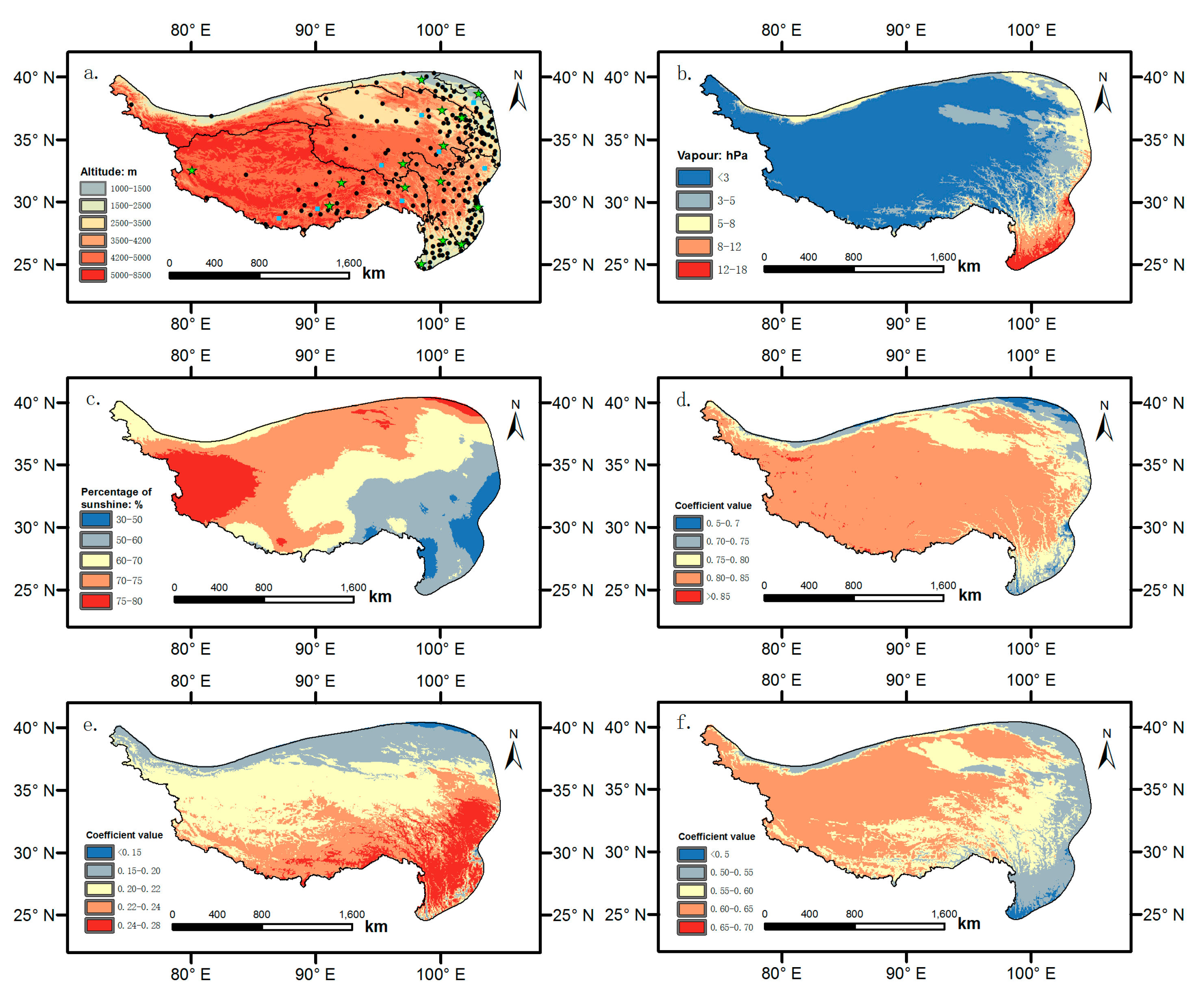
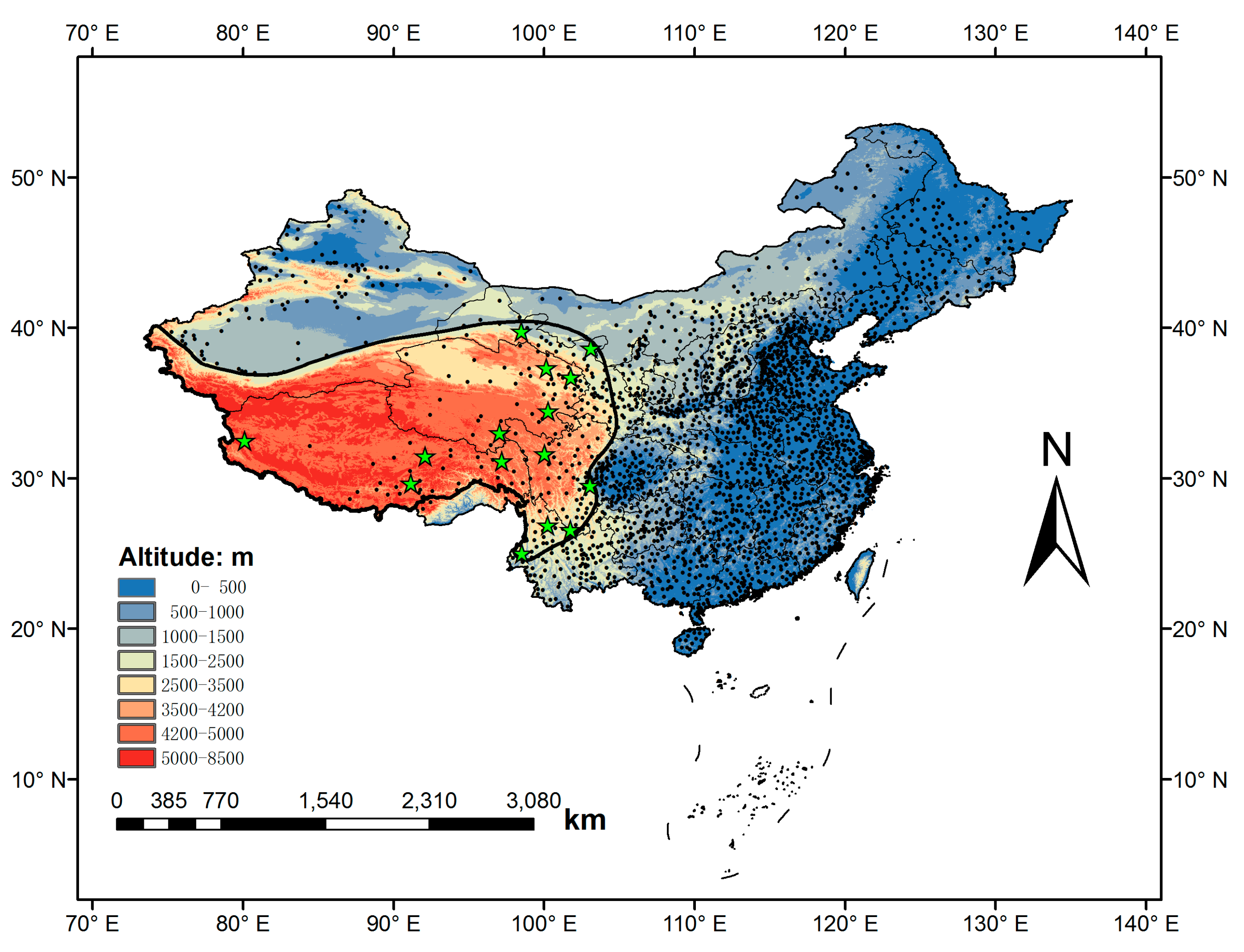
4.1. Study Area and Data Collection

Situated in the Southwest China, the TP is the highest plateau over the world, featuring the tallest mountain Everest at 8844.43 m. The TP belongs to a special Plateau Alpine climate zone, with low temperatures, little precipitation and abundant sunshine [62].
There are about 2400 meteorological stations routinely observing meteorological conditions in China, but most of them are distributed in the east part of the country (Figure 9). Considering that there are very few radiation stations on the TP, the radiation stations in its surrounding regions were also included in this study, aiming to both increase the number of stations and identify the variation of coefficients. The study region defined as in Figure 9 is similar to those in previous studies [52,72]. For accurate estimation of radiation distribution on the TP, the database with 2400 stations archived in the National Meteorological Information Center (NMIC) of China Meteorological Administration (CMA) was employed. Distribution of the solar radiation stations and the routine weather stations is shown in Figure 9. Detailed information about the radiation stations is given in Table 7. A dataset combining the 15 solar radiation stations was first established, including daily solar irradiation, sunshine hours, water vapor pressure, maximum and minimum temperature for the period 1993–2010. Then another dataset was also established for the routine weather stations, including daily sunshine hours and water vapor pressure for the same period. Both datasets were screened similar to rules described by Persaud et al. [73], i.e., daily observations would be excluded from the datasets if (1) any of the observations were missing; and (2) the measured radiation/extra-terrestrial radiation or the actual sunshine hours/potential sunshine hours was greater than 1. The dataset of solar radiation was divided into two sub-datasets. One sub-dataset from 1993 to 2007 was used for model calibration, while the other from 2008 to 2010 was used for model evaluation. The Digital Elevation Model (DEM) data used for generating the gridded climate map was provided by the National Gometic Center of China (NGCC), with spatial resolution of 1 km × 1 km.

4.2. Model Description

In order to elucidate different methods for solar radiation estimation, four types of solar radiation models are defined and described as follows.

4.2.1. Site-Dependent Model

The coefficients of these models are site-dependent. Six site-dependent models, including three sunshine- and three temperature-based ones, were selected to evaluate their performances on the TP and its surrounding regions (Table 8).

4.2.2. Average Model

In order to apply the site-dependent models regionally, two simple methods are suggested. One method is to obtain the regional coefficients by simply averaging coefficients from different radiation stations [45], which can be referred to as “simple-average model”. Another method is to statistically fit the coefficients to a combined database from all the different radiation stations [44,52]. In the view of statistics [45], this method is referred to as “statistical-average model” hereinafter.

4.2.3. Geographical Model

Considering the regional variation in coefficients of the site-dependent models, some researchers tried to establish the relationship between model coefficients and geographical parameters, including latitude, longitude and altitude [30,49,50]. This is referred to as “geographical model” in this work.

4.2.4. Improved Ångström-Type Model

It is assumed that a numerical model based on the radiative transfer theory can be universally applied due to its robust mechanism [11,12]. However, its complex technique in model operation, together with the excessive requirements of input variables, makes it hard for practical application. Thus, models based on the relationship between coefficients and the leading factors accounting for coefficient variations were explored [40], which is referred to as “improved Ångström-type model” in this study.

4.3. Model Evaluation

The Nash-Sutcliffe Efficiency (NSE), the Mean Absolute Percentage Error (MAPE), and the Root Mean Squared Error (RMSE) [30,38,42,52], were used as criteria in evaluating the model performance in this study, and can be described as follows:
N S E = 1 i = 1 n ( O i S i ) 2 i = 1 n ( O i O ¯ ) 2
M A P E = i = 1 n | O i S i | O i × 100 n
R M S E = [ 1 n i = 1 n ( O i S i ) 2 ] 1 2
where O i is the observed value, S i is the simulated value, O ¯ is the average value of the observed radiation, and n is the number of observations. Since MAPE is expressed as percentage whereas RMSE does not, RRMSE is used in place of RMSE for comparison with MAPE. RRMSE is the ration of RMSE to the average value of the observation, which is also expressed as percentage [74]. The greater the NSE and the lower the MAPE and RRMSE, the better the model. Slope and Inter are the slope and intercept of the linear regression between observed and simulated, respectively. The t-test was used to identify significant differences between the results of the selected models [75,76], and the value of t was calculated as [36,40]:
t = ( n 1 ) × M B E 2 ( R M S E 2 M B E 2 )
where MBE was the bias [38,42]:
M B E = 1 n i = 1 n ( S i O i )
When the calculated | t | t 0.05 (critical value), the two groups of data are considered to differ significantly.

4.4. Australia National University SPLINe (ANUSPLIN) Interpolation Method

The ANUSPLIN (version 4.3, Australia National University, Canberra, Australia) was used to spatially interpolate sunshine hours and water vapor pressure in this study, based on which the distribution of the annual mean of daily solar irradiation was rasterized. The ANUSPLIN was developed by the Australian National University in order to provide a facility for transparent analysis and interpolation of noisy multivariate data using thin plate smoothing splines [67]. Given its full consideration of the effect of latitude, longitude and altitude on meteorological interpolation, the method has been more popular than other interpolation methods [68], and a detailed description of ANUSPLIN can be referred in [67,68,69].

5. Conclusions

This study investigated the performance of different site-dependent models based on 15 radiation stations in the TP and its surrounding regions. We found that the coefficients varied greatly among different site-dependent models over the TP, due to the great spatial difference in elevation, water vapor content, complex terrain and also the climate characteristics. The sunshine-based models have better simulation accuracy than temperature-based ones for radiation estimation locally. The simple and statistical average Ångström-based models perform poorly at several stations. The Bristow-based simple/statistical average models perform even worse at most of the stations. Geographical Ångström-type models perform much better than the average models, but it might lead to unacceptable predictions under extreme conditions, as its coefficients are simply fitted by the geographical parameters without any physical foundation.
In order to achieve better performance for estimating solar radiation over the TP, a simple improved Ångström-type model was established using altitude and water vapor pressure as the leading factors accounting for the great variations in the coefficients. The improved model reproduced the coefficients quite well, and has the best performance among all models. Spatial distribution of solar radiation on the TP was then estimated based on the improved Ångström-type model and ANUSPLIN method. The overall pattern of radiation distribution was validated point by point at the 15 solar radiation stations. The estimation showed that solar radiation increases from east to west. Solar radiation in southwest TP is the greatest. Solar radiation estimation results for the TP based on the new model including the coefficients and rasterized solar radiation are available upon request.

Acknowledgments

This research is jointly supported by Special Fund for Meteorology Research in China (GYHY201306048 & GYHY201106024) and the Key Project on the Second Exploration of Meteorological and Energy Conditions on the Tibetan Plateau, and also the National Natural Science Foundation of China (41671107 & 41301092). Deliang Chen is supported by a grant from the Swedish Research Council. We authors are grateful to National Meteorological Information Center for the authorization of access to the full database in this study. Special thank is also due to the weathermen working hard on the Tibetan Plateau under altitude hypoxia conditions.

Author Contributions

Tao Pan and Jiandong Liu conceived and designed the experiments; Jiandong Liu performed the experiments; Jiandong Liu and Tao Pan analyzed the data; Deliang Chen, Xiuji Zhou, Qiang Yu, Gerald N. Flerchinger, De Li Liu, Xintong Zou, Hans W. Linderholm, Jun Du, Dingrong Wu and Yanbo Shen contributed data/materials/analysis methods and discussion; Jiandong Liu wrote the paper.

Conflicts of Interest

The authors declare no conflict of interest.

References

  1. Yaghoubi, M.A.; Sabzevari, A. Further data on solar radiation in Shiraz, Iran. Renew. Energy 1996, 7, 393–399. [Google Scholar] [CrossRef]
  2. Colak, I.; Sagiroglu, S.; Demirtas, M.; Yesilbudak, M. A data mining approach: Analyzing wind speed and insolation period data in Turkey for installations of wind and solar power plants. Energy Convers. Manag. 2013, 65, 185–197. [Google Scholar] [CrossRef]
  3. Wong, L.T.; Chow, W.K. Solar radiation model. Appl. Energy 2001, 69, 191–224. [Google Scholar] [CrossRef]
  4. Yue, C.D.; Huang, G.R. An evaluation of domestic solar energy potential in Taiwan incorporating land use analysis. Energy Policy 2011, 39, 7988–8002. [Google Scholar] [CrossRef]
  5. Abraha, M.G.; Savage, M.J. Comparison of estimates of daily solar radiation from air temperature range for application in crop simulations. Agric. For. Meteorol. 2008, 148, 401–416. [Google Scholar] [CrossRef]
  6. Hunt, L.A.; Kuchar, L.S.; Swanton, C.J. Estimation of solar radiation for use in crop modeling. Agric. For. Meteorol. 1998, 91, 293–300. [Google Scholar] [CrossRef]
  7. Cristea, N.C.; Kampf, S.K.; Burges, S.J. Linear models for estimating annual and growing season reference evapotranspiration using averages of weather variables. Int. J. Climatol. 2013, 33, 376–387. [Google Scholar] [CrossRef]
  8. Kang, M.S.; Park, S.W.; Lee, J.J.; Yoo, K.H. Applying SWAT for TMDL programs to a small watershed containing rice paddy fields. Agric. Water Manag. 2006, 79, 72–92. [Google Scholar] [CrossRef]
  9. Allen, R.G.; Pereira, L.S.; Raes, D.; Smith, M. Crop Evapotranspiration-Guidelines for Computing Crop Water Requirements; FAO Irrigation and Drainage Paper 56; Food and Agriculture Organization of the United Nations: Rome, Italy, 1998; Volume 300, p. D05109. [Google Scholar]
  10. Weiss, A.; Hays, C.J. Simulation of daily solar irradiance. Agric. For. Meteorol. 2004, 123, 187–199. [Google Scholar] [CrossRef]
  11. Morcrette, J.J.; Mozdzynski, G.; Leutbecher, M. A reduced radiation grid for the ECMWF integrated forecasting system. Mon. Weather Rev. 2008, 136, 4760–4772. [Google Scholar] [CrossRef]
  12. Manners, J.; Thelen, J.C.; Petch, J.; Hill, P.; Edwards, J.M. Two fast radiative transfer methods to improve the temporal sampling of clouds in numerical weather prediction and climate models. Q. J. R. Meteorol. Soc. 2009, 135, 457–468. [Google Scholar] [CrossRef]
  13. Tymvios, F.S.; Jacovides, C.P.; Michaelides, S.C.; Scouteli, C. Comparative study of Angstrom’s and artificial neural network’s methodologies in estimating global solar radiation. Sol. Energy 2005, 70, 752–762. [Google Scholar] [CrossRef]
  14. Jacovides, C.P.; Tymvios, F.S.; Boland, J.; Tsitouri, M. Artificial Neural Network models for estimating daily solar global UV, PAR and broadband radiant fluxes in an eastern Mediterranean site. Atmos. Res. 2015, 152, 138–145. [Google Scholar] [CrossRef]
  15. Fadare, D.A. Modelling of solar energy potential in Nigeria using an artificial neural network model. Appl. Energy 2009, 86, 1410–1422. [Google Scholar] [CrossRef]
  16. Şenkal, O.; Kuleli, T. Estimation of solar radiation over Turkey using artificial neural network and satellite data. Appl. Energy 2009, 86, 1222–1228. [Google Scholar] [CrossRef]
  17. Mihalakakou, G.; Santamouris, M.; Asimakopoulos, D.N. The total solar radiation time series simulation in Athens, using neural networks. Theor. Appl. Climatol. 2000, 66, 185–197. [Google Scholar] [CrossRef]
  18. Qin, J.; Chen, Z.; Yang, K.; Liang, S.; Tang, W. Estimation of monthly-mean daily global solar radiation based on MODIS and TRMM products. Appl. Energy 2011, 88, 2480–2489. [Google Scholar] [CrossRef]
  19. Janjai, S.; Pankaew, P.; Laksanaboonsong, J. A model for calculating hourly global solar radiation from satellite data in the tropics. Appl. Energy 2009, 86, 1450–1457. [Google Scholar] [CrossRef]
  20. Hinkelman, L.M.; Stackhouse, P.W., Jr.; Wielicki, B.A.; Zhang, T.; Wilson, S.R. Surface insolation trends from satellite and ground measurements: Comparisons and challenges. J. Geophys. Res. Atmos. 2009, 114, 4427–4433. [Google Scholar] [CrossRef]
  21. Pinker, R.T.; Frouin, R.; Li, Z. A review of satellite methods to derive surface shortwave irradiance. Remote Sens. Environ. 1995, 51, 108–124. [Google Scholar] [CrossRef]
  22. Boilley, A.; Wald, L. Comparison between meteorological re-analyses from ERA-Interim and MERRA and measurements of daily solar irradiation at surface. Renew. Energy 2015, 75, 135–143. [Google Scholar] [CrossRef]
  23. Ångström, A. Solar and terrestrial radiation. Q. J. R. Met. Soc. 1924, 50, 121–125. [Google Scholar]
  24. Prescott, J. Evaporation from a water surface in relation to solar radiation. Trans. R. Soc. S. Aust. 1940, 64, 114–118. [Google Scholar]
  25. Ögelman, H.; Ecevit, A.; Tasdemiroǧlu, E. A new method for estimating solar radiation from bright sunshine data. Sol. Energy 1984, 33, 619–625. [Google Scholar] [CrossRef]
  26. Bahel, V.; Bakhsh, H.; Srinivasan, R. A correlation for estimation of global solar radiation. Energy 1987, 12, 131–135. [Google Scholar] [CrossRef]
  27. Ampratwum, D.B.; Dorvlo, A.S.S. Estimation of solar radiation from the number of sunshine hours. Appl. Energy 1999, 63, 161–167. [Google Scholar] [CrossRef]
  28. Bristow, K.L.; Campbell, G.S. On the relationship between incoming solar radiation and daily maximum and minimum temperature. Agric. For. Meteorol. 1984, 31, 159–166. [Google Scholar] [CrossRef]
  29. Hargreaves, G.L.; Hargreaves, G.H.; Riley, J.P. Irrigation water requirements for Senegal River Basin. J. Irrig. Drain. Eng. 1985, 111, 265–275. [Google Scholar] [CrossRef]
  30. Chen, R.; Kang, E.; Yang, J.; Lu, S.; Zhao, W. Validation of five global radiation models with measured daily data in China. Energy Convers. Manag. 2004, 45, 1759–1769. [Google Scholar] [CrossRef]
  31. Meza, F.; Varas, E. Estimation of mean monthly solar global radiation as a function of temperature. Agric. For. Meteorol. 2000, 100, 231–241. [Google Scholar] [CrossRef]
  32. Goodin, D.G.; Hutchinson, J.M.S.; Vanderlip, R.L.; Knapp, M.C. Estimating solar irradiance for crop modeling using daily air temperature data. Agron. J. 1999, 91, 845–851. [Google Scholar] [CrossRef]
  33. Weiss, A.; Hays, C.J.; Hu, Q.; Easterling, W.E. Incorporating bias error in calculating solar irradiance: Implications for crop yield simulations. Agron. J. 2001, 93, 1321–1326. [Google Scholar] [CrossRef]
  34. Liu, D.L.; Scott, B.J. Estimation of solar radiation in Australia from rainfall and temperature observations. Agric. For. Meteorol. 2001, 106, 41–59. [Google Scholar] [CrossRef]
  35. Mccaskill, M.R. Prediction of solar radiation from rainday information using regionally stable coefficients. Agric. For. Meteorol. 1990, 51, 247–255. [Google Scholar] [CrossRef]
  36. Wu, G.; Liu, Y.; Wang, T. Methods and strategy for modeling daily global solar radiation with measured meteorological data—A case study in Nanchang station, China. Energy Convers. Manag. 2007, 48, 2447–2452. [Google Scholar] [CrossRef]
  37. Podestá, G.P.; Núñez, L.; Villanueva, C.A.; Skansi, M.A.A. Estimating daily solar radiation in the Argentine Pampas. Agric. For. Meteorol. 2004, 123, 41–53. [Google Scholar] [CrossRef]
  38. Liu, J.; Liu, J.; Linderholm, H.W.; Chen, D.; Yu, Q.; Wu, D.; Haginoya, S. Observation and calculation of the solar radiation on the Tibetan Plateau. Energy Convers. Manag. 2012, 57, 23–32. [Google Scholar] [CrossRef]
  39. Moradi, I.; Mueller, R.; Perez, R. Retrieving daily global solar radiation from routine climate variables. Theor. Appl. Climatol. 2014, 116, 661–669. [Google Scholar] [CrossRef]
  40. Liu, X.; Xu, Y.; Zhong, X.; Zhang, W.; Porter, J.R.; Liu, W. Assessing models for parameters of the Ångström-Prescott formula in China. Appl. Energy 2012, 327–338. [Google Scholar] [CrossRef]
  41. Liu, X.; Mei, X.; Li, Y.; Wang, Q.; Jensraunsø, J.; Zhang, Y.; Johnroy, P. Evaluation of temperature-based global solar radiation models in China. Agric. For. Meteorol. 2009, 149, 1433–1446. [Google Scholar] [CrossRef]
  42. Liu, X.; Mei, X.; Li, Y.; Porter, J.R.; Wang, Q.; Zhang, Y. Choice of the Ångström–Prescott coefficients: Are time-dependent ones better than fixed ones in modeling global solar irradiance? Energy Convers. Manag. 2010, 51, 2565–2574. [Google Scholar] [CrossRef]
  43. Wu, D.; Qiang, Y.; Lu, C.; Hengsdijk, H. Quantifying production potentials of winter wheat in the North China Plain. Eur. J. Agron. 2006, 24, 226–235. [Google Scholar] [CrossRef]
  44. Wu, Z.; Du, H.; Zhao, D.; Ming, L. Estimating daily global solar radiation during the growing season in Northeast China using the Ångström–Prescott model. Theor. Appl. Climatol. 2012, 108, 495–503. [Google Scholar] [CrossRef]
  45. Von Storch, H.; Zwiers, F.W. Statistical Analysis in Climate Research; Cambridge University Press: Cambridge, UK, 2001; pp. 3–10. [Google Scholar]
  46. Chen, R.; Lu, S.; Kang, E.; Yang, J.; Ji, X. Estimating daily global radiation using two types of revised models in China. Energy Convers. Manag. 2006, 47, 865–878. [Google Scholar]
  47. Zhou, J.; Wu, Y.; Gang, Y. General formula for estimation of monthly average daily global solar radiation in China. Energy Convers. Manag. 2005, 46, 257–268. [Google Scholar]
  48. Wu, W.; Liu, H.B. Assessment of monthly solar radiation estimates using support vector machines and air temperatures. Int. J. Climatol. 2012, 32, 274–285. [Google Scholar] [CrossRef]
  49. Li, M.F.; Tang, X.P.; Wu, W.; Liu, H.B. General models for estimating daily global solar radiation for different solar radiation zones in Mainland China. Energy Convers. Manag. 2013, 70, 139–148. [Google Scholar] [CrossRef]
  50. Li, M.F.; Fan, L.; Liu, H.B.; Guo, P.T.; Wu, W. A general model for estimation of daily global solar radiation using air temperatures and site geographic parameters in Southwest China. J. Atmos. Sol. Terr. Phys. 2013, 92, 145–150. [Google Scholar] [CrossRef]
  51. Wang, Q.; Qiu, H.N. Situation and outlook of solar energy utilization in Tibet, China. Renew. Sustain. Energy Rev. 2009, 13, 2181–2186. [Google Scholar] [CrossRef]
  52. Pan, T.; Wu, S.; Dai, E.; Liu, Y. Estimating the daily global solar radiation spatial distribution from diurnal temperature ranges over the Tibetan Plateau in China. Appl. Energy 2013, 107, 384–393. [Google Scholar] [CrossRef]
  53. Li, H.; Ma, W.; Lian, Y.; Wang, X.; Zhao, L. Global solar radiation estimation with sunshine duration in Tibet, China. Renew. Energy 2011, 36, 3141–3145. [Google Scholar] [CrossRef]
  54. Liou, K. An introduction to Atmospheric Radiation, 2nd ed.; Elsevier Science: San Diego, CA, USA, 2002. [Google Scholar]
  55. Dai, J. The Climate over the Tibetan Plateau; Meteorological Press: Beijing, China, 1990. (In Chinese) [Google Scholar]
  56. Liu, J.; Sun, Z.; Liang, H.; Xu, X.; Wu, P. Precipitable water vapor on the Tibetan Plateau estimated by GPS, water vapor radiometer, radiosonde, and numerical weather prediction analysis and its impact on the radiation budget. J. Geophys. Res. Atmos. 2005, 110. [Google Scholar] [CrossRef]
  57. Yang, K.; Huang, G.W.; Tamai, N. A hybrid model for estimating global solar radiation. Sol. Energy 2001, 70, 13–22. [Google Scholar] [CrossRef]
  58. Streets, D.G.; Yu, C.; Wu, Y.; Chin, M.; Zhao, Z.; Hayasaka, T.; Shi, G. Aerosol trends over China, 1980–2000. Atmos. Res. 2008, 88, 174–182. [Google Scholar] [CrossRef]
  59. Zhou, X.; Luo, C. Ozone valley over Tibetan Plateau. Acta Meteorol. Sin. 1994, 8, 505–506. [Google Scholar]
  60. Yu, Q.; Liu, Y.; Liu, J.; Wang, T. Simulation of leaf photosynthesis of winter wheat on Tibetan Plateau and in North China plain. Ecol. Model. 2002, 155, 205–216. [Google Scholar] [CrossRef]
  61. Arya, S. Introduction to Micrometeorology; Academic Press: San Diego, CA, USA, 2001. [Google Scholar]
  62. Domrös, M.; Peng, G. The Climate of China; Springer: Berlin/Heidelberg, Germany, 1988; pp. 258–278. [Google Scholar]
  63. Yang, K.; Ding, B.; Qin, J.; Tang, W.; Lu, N.; Lin, C. Can aerosol loading explain the solar dimming over the Tibetan Plateau? Geophys. Res. Lett. 2012, 39. [Google Scholar] [CrossRef]
  64. Wang, B.; Zhang, G.; Li, L. Thesis on Wind and Solar Energy in China; Meteorological Press: Beijing, China, 2008. (In Chinese) [Google Scholar]
  65. Wang, Y.; Yang, Y.; Han, S.; Wang, Q.; Zhang, J. Sunshine dimming and brightening in Chinese cities (1955–2011) was driven by air pollution rather than clouds. Clim. Res. 2013, 56, 11–20. [Google Scholar] [CrossRef]
  66. Zhao, N.; Zeng, X.; Han, S. Solar radiation estimation using sunshine hour and air pollution index in China. Energy Convers. Manag. 2013, 76, 846–851. [Google Scholar] [CrossRef]
  67. Hutchinson, M.F. ANUSPLIN Version 4.36 User Guide; The Australia Nationaluniversity, Center for Resource and Environment Studies: Canberra, Australia, 2006. [Google Scholar]
  68. Price, D.T.; Mckenney, D.W.; Nalder, I.A.; Hutchinson, M.F.; Kesteven, J.L. A comparison of two statistical methods for spatial interpolation of Canadian monthly mean climate data. Agric. For. Meteorol. 2000, 101, 81–94. [Google Scholar] [CrossRef]
  69. Hijmans, R.J.; Cameron, S.E.; Parra, J.L.; Jones, P.G.; Jarvis, A. Very high resolution interpolated climate surfaces for global land areas. Int. J. Climatol. 2005, 25, 1965–1978. [Google Scholar] [CrossRef]
  70. Wu, J.; Gao, X. A gridded daily observation dataset over China region and comparison with the other datasets. Chin. J. Geophys. 2013, 56, 1102–1111. (In Chinese) [Google Scholar]
  71. Lefèvre, M.; Oumbe, A.; Blanc, P.; Espinar, B.; Gschwind, B.; Qu, Z.; Wald, L.; Schroedter-Homscheidt, M.; Hoyer-Klick, C.; Arola, A.; et al. McClear: A new model estimating downwelling solar radiation at ground level in clear-sky condition. Atmos. Meas. Tech. 2013, 6, 2403–2418. [Google Scholar] [CrossRef]
  72. Zhang, Y.; Liu, C.; Tang, Y.; Yang, Y. Trends in pan evaporation and reference and actual evapotranspiration across the Tibetan Plateau. J. Geophys. Res. Atmos. 2007, 112, 113–120. [Google Scholar] [CrossRef]
  73. Persaud, N.; Lesolle, D.; Ouattara, M. Coefficients of the Ångström-Prescott equation for estimating global irradiance from hours of bright sunshine in Botswana and Niger. Agric. For. Meteorol. 1997, 88, 27–35. [Google Scholar] [CrossRef]
  74. Willmott, C.T.; Matsuura, K. Advantages of the mean absolute error (MAE) over the root mean square error (RMSE) in assessing average model performance. Clim. Res. 2005, 30, 79–82. [Google Scholar] [CrossRef]
  75. Stone, R.J. Improved statistical procedure for the evaluation of solar radiation estimation models. Sol. Energy 1993, 51, 289–291. [Google Scholar] [CrossRef]
  76. Jacovides, C.P.; Kontoyiannis, H. Statistical procedures for the evaluation of evapotranspiration computing models. Agric. Water Manag. 1995, 27, 365–371. [Google Scholar] [CrossRef]
Figure 1. Variation of annual mean of daily solar irradiation on the Tibetan Plateau and its surrounding regions.
Energies 10 00892 g001
Figure 2. Values of t-statistic test between and within the results from the sunshine- and temperature-based model. S1, S2, S3 denote the sunshine-based model Angstrom, Ogelman and Bahell, respectively. T1, T2, T3 denote the temperature-based model Bristow, Hargreaves and Chen, respectively.
Energies 10 00892 g002
Figure 3. Variation in coefficients of the site-dependent Ångström model.
Energies 10 00892 g003
Figure 4. Relationship between coefficients in the Ångström model and the leading factors related to (a) altitude (m), and (b) water vapor pressure (hPa).
Energies 10 00892 g004
Figure 5. Performance of different models in predicting daily solar irradiation in Lhasa from 2008 to 2010. The horizontal axis denotes observation values, and the vertical axis prediction values (unit: MJ·m−2).
Energies 10 00892 g005
Figure 6. Validation of the ANUSPLIN method in interpolating (a) water vapor pressure and (b) sunshine percentage over the Tibetan Plateau and its surrounding regions.
Energies 10 00892 g006
Figure 7. Distribution of weather stations, the interpolated meteorological variables and the rasterized coefficients of the Ångström model. (a) Distribution of weather stations, stars denote radiation stations, dots the weather stations, and squares weather station used for validation of ANUSPLIN method, (b) annual mean water vapor pressure (unit: hPa), (c) annual mean sunshine percentage, (d) coefficient (a + b), (e) coefficient a, and (f) coefficient b.
Energies 10 00892 g007
Figure 8. Spatial distribution of the annual mean of daily solar irradiation over the Tibetan Plateau. (a) Extra-terrestrial radiation, (b) Annual mean of daily solar irradiation, and the seasonal mean of daily solar irradiation in (c) spring, (d) summer, (e) autumn, and (f) winter (unit: MJ·m−2).
Energies 10 00892 g008
Figure 9. Distribution of solar radiation and weather stations. The black dots denote weather stations, and the five-point stars denote solar radiation stations used in this study.
Energies 10 00892 g009
Table 1. Calibration of the sunshine- and temperature-based site-dependent models at different locations using data from 1993 to 2007 in this study.
Sunshine-Based ModelsStationabcdNSEMAPERRMSESlopeIntern
AngstromJiuquan0.2190.514--0.9488.62910.0040.9011.5475469
Minqin0.1930.541--0.9517.6479.3330.9301.1615466
Gangcha0.1980.603--0.9158.53011.0220.9411.1295430
Xining0.2150.530--0.9369.68111.3010.9041.4635458
Shiquanhe0.2290.616--0.8568.13811.4480.8902.5785433
Naqu0.2710.574--0.8189.70613.0950.8972.1035294
Lhasa0.2830.530--0.8856.8568.9580.8832.3715283
Yushu0.2290.560--0.9139.10310.8370.9191.3975473
Guoluo0.2470.563--0.8889.50612.1070.9171.5465456
Changdu0.2180.592--0.8719.38611.8280.8831.9735468
Ganzi0.2910.511--0.8848.63011.0700.8722.3185068
Ermeishan0.2340.565--0.82618.27521.3270.8871.6595472
Lijiang0.2220.538--0.8919.99111.3030.8702.1705440
Panzhihua0.1730.498--0.88311.28713.2180.8572.2015475
Tengchong0.2150.506--0.81013.12715.5340.8272.6485471
Average0.2290.549--0.8859.89912.1590.8921.1845410
OgelmanJiuquan0.2270.4680.044-0.9488.54110.0100.9001.5625469
Minqin0.2030.4820.056-0.9517.6199.3330.9291.1965466
Gangcha0.1990.5960.007-0.9158.52711.0220.9411.1325430
Xining0.2030.628−0.110-0.9389.70911.1150.9061.4235458
Shiquanhe0.2710.4590.124-0.8568.16811.4210.8882.6415433
Naqu0.2860.5040.064-0.8189.68213.0910.8942.1755294
Lhasa0.2720.575−0.038-0.8856.8418.9490.8872.3095283
Yushu0.2550.4230.137-0.9148.98010.7410.9241.3155473
Guoluo0.2610.4750.088-0.8889.50212.0710.9121.6305456
Changdu0.2550.3860.217-0.8749.21911.6890.8782.0675468
Ganzi0.2810.568−0.057-0.8858.63511.0280.8762.2405068
Ermeishan0.2340.574−0.010-0.82618.27721.3510.8881.6645472
Lijiang0.2170.573−0.035-0.89210.05911.2750.8752.0985440
Panzhihua0.1670.544−0.048-0.88311.30713.1760.8582.1805475
Tengchong0.2160.4970.010-0.81013.10615.5380.8262.6625471
Average0.2360.5170.030-0.8869.87812.1210.8921.8865410
BahellJiuquan0.2200.593−0.2810.2180.9488.61610.0030.9001.5495469
Minqin0.1940.642−0.3480.2630.9517.6169.3250.9281.1925466
Gangcha0.1880.766−0.4090.2690.9168.49010.9710.9411.1435430
Xining0.1920.923−0.9680.6290.9409.64510.9650.9111.3465458
Shiquanhe0.2360.827−0.6700.4730.8588.19111.3650.8872.6795433
Naqu0.2810.554−0.0520.0740.8189.67413.0820.8932.1955294
Lhasa0.2630.651−0.2060.1050.8856.8378.9450.8852.3185283
Yushu0.2530.4540.0610.0530.9149.00010.7440.9261.3065473
Guoluo0.2510.649−0.3730.3160.8899.42912.0010.9111.6355456
Changdu0.2330.683−0.6030.6140.8769.12211.6060.8822.0165468
Ganzi0.2720.698−0.3950.2330.8868.66710.9930.8772.2415068
Ermeishan0.2300.775−0.6500.4690.82818.23621.1860.8871.6775472
Lijiang0.2020.827−0.7260.4770.8949.98411.1440.8712.1265440
Panzhihua0.1500.954−1.1930.8050.88811.06512.9120.8701.9915475
Tengchong0.2030.787−0.8340.6040.81613.12415.2940.8242.6695471
Average0.2250.719−0.5100.3730.8879.84612.0360.8931.8725410
Temperature-Based ModelsStationabcdNSEMAPERRMSESlopeIntern
BristowJiuquan0.7580.0361.423-0.75514.46721.7190.8043.5275469
Minqin0.7130.0251.650-0.70514.15522.7780.7774.1595466
Gangcha0.7410.0052.340-0.66115.10921.9890.7194.9655429
Xining0.6900.0221.607-0.74914.34522.4410.7384.1665458
Shiquanhe0.8560.0271.610-0.72311.59315.8770.7745.3515433
Naqu0.9030.0451.245-0.51916.62021.2850.6207.4525294
Lhasa0.7690.0121.974-0.66111.63915.3770.7405.5815283
Yushu0.7220.0281.496-0.70116.11120.0490.6625.7415473
Guoluo0.7350.0251.560-0.65516.93721.2110.6765.8015456
Changdu1.0050.0301.181-0.68614.73918.4640.6885.1645468
Ganzi0.7850.0261.512-0.72313.68817.0920.7524.7095068
Ermeishan0.8160.0411.531-0.58323.50833.0290.6714.5685472
Lijiang0.7600.0141.878-0.67916.13019.3950.7334.4495440
Panzhihua0.6010.0102.123-0.66416.20522.3770.6425.6935475
Tengchong0.9170.0571.118-0.61918.36321.9910.6994.7255471
Average0.7850.0271.617-0.67215.57421.0050.7135.0705410
HargreavesJiuquan0.184−0.102--0.77614.49920.7420.8243.1795469
Minqin0.172−0.050--0.72214.73722.1130.7824.0405466
Gangcha0.242−0.251--0.69214.90920.9580.7394.8325429
Xining0.175−0.136--0.75914.74721.9960.7344.1265458
Shiquanhe0.1630.106--0.71112.08216.1920.7585.6805433
Naqu0.175−0.032--0.50417.41021.6270.6247.4655294
Lhasa0.188−0.047--0.65112.35015.6210.7086.0545283
Yushu0.155−0.038--0.68616.83220.5540.6535.9175473
Guoluo0.151−0.010--0.61918.22622.2680.6316.5595456
Changdu0.182−0.175--0.67315.14318.8240.6965.2485468
Ganzi0.185−0.115--0.71214.17317.4250.7404.8645068
Ermeishan0.282−0.306--0.62223.52631.4510.6804.4375472
Lijiang0.258−0.321--0.66216.77719.9160.6955.3395440
Panzhihua0.214−0.257--0.64916.58522.8580.5986.2475475
Tengchong0.212−0.192--0.62518.20321.8110.7034.6625471
Average0.193−0.128--0.67116.01320.9570.7045.2435410
ChenJiuquan0.312−0.231--0.77714.49220.7170.8213.2185469
Minqin0.300−0.191--0.72814.39721.8890.7883.9245466
Gangcha0.406−0.409--0.70014.69020.6720.7634.4695429
Xining0.302−0.263--0.76414.32021.7730.7513.9755458
Shiquanhe0.301−0.072--0.71412.05816.1270.7705.4635433
Naqu0.319−0.211--0.50817.35921.5380.6387.1995294
Lhasa0.345−0.248--0.65912.15715.4400.7255.7355283
Yushu0.282−0.195--0.68916.66320.4320.6635.7475473
Guoluo0.281−0.174--0.63517.62321.8130.6616.0225456
Changdu0.337−0.374--0.67315.27918.8370.7085.0395468
Ganzi0.335−0.296--0.72013.87917.2060.7584.5815068
Ermeishan0.357−0.233--0.59624.94032.4910.6834.5015472
Lijiang0.393−0.397--0.66216.69919.9200.7174.9245440
Panzhihua0.332−0.330--0.65716.15922.6160.6205.9575475
Tengchong0.293−0.179--0.60719.14722.3170.7144.5045471
Average0.326−0.254--0.67315.99120.9190.7195.0175410
Table 2. Validation of the sunshine- and temperature-based site-dependent models for the calibrated coefficients in Table 1 using data from 2008 to 2010 at different locations in this study.
Sunshine-Based ModelsStationNSEMAPERRMSESlopeIntern
AngtromJiuquan0.9499.88610.4740.9181.6401095
Minqin0.9588.6039.1010.9251.4901096
Gangcha0.9357.9379.2110.996−0.1231096
Xining0.9269.91911.6150.9081.4141095
Shiquanhe0.9006.9568.8960.9720.3361090
Naqu0.8728.72310.3440.9401.3871094
Lhasa0.8916.7728.5100.9192.1741094
Yushu0.81515.47616.7100.8792.871731
Guoluo0.81310.89515.6720.8892.4011095
Changdu0.80114.12815.5510.8723.1151094
Ganzi0.9148.2269.5820.8782.2081096
Ermeishan0.87616.95217.7670.8901.6791096
Lijiang0.83811.84013.5550.8902.0741096
Panzhihua0.70020.53522.4530.7024.2361096
Tengchong0.78114.39515.9430.8853.0371096
Average0.86511.41613.0260.8981.9961070
OgelmanJiuquan0.9499.82510.4140.9191.6511095
Minqin0.9588.3559.0840.9251.4991096
Gangcha0.9357.9359.2120.995−0.1171096
Xining0.92710.14311.5120.9081.3591095
Shiquanhe0.9026.8638.8270.9670.4771090
Naqu0.8728.74110.3460.9361.4711094
Lhasa0.8906.7958.5370.9212.1421094
Yushu0.81815.41816.5930.8822.833731
Guoluo0.81410.95215.6280.8802.5311095
Changdu0.80114.06315.5500.8643.2451094
Ganzi0.9148.1349.5320.8842.1001096
Ermeishan0.87516.97517.7990.8911.6851096
Lijiang0.83612.13113.6270.8961.9821096
Panzhihua0.69920.47522.4830.7024.2331096
Tengchong0.78114.38215.9180.8853.0351096
Average0.86511.41213.0040.8972.0081070
BahellJiuquan0.9499.92410.4150.9211.6121095
Minqin0.9598.5649.0380.9251.4921096
Gangcha0.9367.9009.1780.996−0.1181096
Xining0.9309.77811.2890.9161.2691095
Shiquanhe0.9036.8618.7780.9630.5771090
Naqu0.8728.73610.3380.9341.5011094
Lhasa0.8916.8598.5010.9192.1651094
Yushu0.81615.48316.6830.8852.827731
Guoluo0.81310.94015.6370.8772.5921095
Changdu0.80114.19915.5510.8683.2151094
Ganzi0.9158.0959.5010.8842.1101096
Ermeishan0.87816.72217.6170.8851.7541096
Lijiang0.84212.01613.3790.8971.9511096
Panzhihua0.70120.48822.4070.7124.0741096
Tengchong0.78814.42515.6750.8743.1731096
Average0.86611.39912.9320.8972.0131070
Temperature-Based ModelsStationNSEMAPERRMSESlopeIntern
BristowJiuquan0.77014.85522.1530.8173.3481095
Minqin0.71714.70723.7080.7784.2241096
Gangcha0.69515.15719.9970.7764.0721096
Xining0.75313.42021.1900.7564.0771095
Shiquanhe0.76610.49713.6210.8254.1541090
Naqu0.57515.82318.8600.6676.4651094
Lhasa0.69410.96414.2290.7535.3981094
Yushu0.65720.46922.7670.6446.141731
Guoluo0.56618.11223.8340.6606.2831095
Changdu0.68417.80319.6000.6955.5331094
Ganzi0.74613.51616.4290.7554.5051096
Ermeishan0.64822.50729.9020.6754.4161096
Lijiang0.57518.44921.9230.7365.3451096
Panzhihua0.47622.95129.6560.4898.0161096
Tengchong0.59118.53821.7790.7444.3441096
Average0.66116.51821.3100.7185.0881070
HargreavesJiuquan0.79714.73220.8110.8373.0501095
Minqin0.73014.99923.1290.7744.2301096
Gangcha0.72515.08918.9770.7924.0181096
Xining0.75913.94420.9070.7524.0541095
Shiquanhe0.73511.17714.4850.8044.6461090
Naqu0.54416.75419.5460.6636.6191094
Lhasa0.68411.63114.4720.7145.9991094
Yushu0.62821.70123.7050.6206.619731
Guoluo0.53219.65924.7560.6137.0991095
Changdu0.66618.48320.1520.7125.4961094
Ganzi0.75213.90416.2250.7474.6091096
Ermeishan0.67722.55128.6120.6884.1971096
Lijiang0.49220.90923.9830.7066.2131096
Panzhihua0.48622.95929.3880.4738.1431096
Tengchong0.60118.05621.5140.7534.2221096
Average0.65417.10321.3770.7105.2811070
ChenJiuquan0.79714.52120.7870.8363.0041095
Minqin0.73414.71522.9760.7844.0691096
Gangcha0.73214.78718.7210.8163.6671096
Xining0.76213.72320.7890.7673.8841095
Shiquanhe0.73811.07014.4170.8184.3421090
Naqu0.54516.72519.5310.6836.2541094
Lhasa0.69111.55314.3070.7335.6451094
Yushu0.63221.36823.5720.6366.374731
Guoluo0.54418.87324.4300.6436.5961095
Changdu0.66318.46020.2360.7335.1711094
Ganzi0.76313.30115.8540.7724.2041096
Ermeishan0.65523.90729.6070.6884.2611096
Lijiang0.50220.27523.7360.7145.9461096
Panzhihua0.48822.85829.3110.4818.0501096
Tengchong0.56919.43322.3540.7644.0331096
Average0.65417.03821.3750.7255.0331070
Table 3. Performance of the simple average model and the statistical average model using the validation dataset from 2008 to 2010. (A) Simple average model. Angstrom-Based model: a = 0.229, b = 0.549; Browstow-Based model: a = 0.785, b = 0.027, c = 1.617. (B) Statistical average model. Angstrom-based model: a = 0.229, b = 0.550; Browstow-Based model: a = 0.757, b = 0.044, c = 1.373.
(A)
StationAngstrom-Based ModelBristow-Based Model
NSEMAPERRMSESlopeInternNSEMAPERRMSESlopeIntern
Jiuquan0.92212.70712.8740.9761.69210950.65617.05527.0510.9023.9171095
Minqin0.92311.95012.3680.9711.93810960.61816.60327.5140.8524.6811096
Gangcha0.9358.3199.2210.9500.58110960.66715.82220.8720.7365.2831096
Xining0.91410.31512.4760.9461.57010950.38123.43633.5530.8815.7001095
Shiquanhe0.81310.63512.1650.8910.52410900.70413.21715.3230.7603.8411090
Naqu0.80311.04312.8500.8760.81110940.51217.04520.2160.7026.7291094
Lhasa0.8737.2269.1580.8871.51510940.69711.03114.1650.7265.7651094
Yushu0.82515.18816.2790.8652.8967310.24129.87933.8540.7557.800731
Guoluo0.82310.97515.2240.8592.11310950.25423.07031.2580.7347.6181095
Changdu0.82913.33514.3980.8333.3651094−0.34035.83540.3640.8447.9291094
Ganzi0.85210.01412.5260.8750.94010960.57417.31121.2760.8125.6821096
Ermeishan0.87516.92117.8250.8651.67910960.53227.52034.4540.6282.6701096
Lijiang0.82112.76614.2280.9092.19210960.46320.61224.6530.6917.0321096
Panzhihua0.59621.46226.0310.7875.72210960.27822.46834.8090.55510.3521096
Tengchong0.58620.13621.9100.9603.15310960.42121.46625.8980.9132.6891096
Average0.82612.86614.6360.8972.04610700.44420.82527.0170.7665.8461070
(B)
StationAngstrom-Based ModelBristow-Based Model
NSEMAPERRMSESlopeInternNSEMAPERRMSESlopeIntern
Jiuquan0.92112.79112.9540.9771.69010950.75514.53622.8480.8213.7261095
Minqin0.92212.05112.4560.9721.93610960.71214.46123.8820.7754.4411096
Gangcha0.9358.2899.2010.9510.57610960.65317.30121.3140.6615.1471096
Xining0.91410.36512.5190.9471.56610950.60516.58626.8070.7995.5171095
Shiquanhe0.81610.55712.0860.8920.52210900.48317.77720.2530.6903.7131090
Naqu0.80510.98612.7870.8770.80510940.55416.50219.3330.6316.4661094
Lhasa0.8757.1829.1120.8881.51410940.60212.81416.2290.6555.5261094
Yushu0.82415.21216.3140.8672.8947310.51024.99427.2070.6827.381731
Guoluo0.82310.96215.2180.8602.10810950.47820.00226.1380.6617.3761095
Changdu0.82913.36714.4330.8343.36310940.20427.99231.1150.7677.4751094
Ganzi0.8539.96512.4720.8770.93410960.71614.60217.3740.7315.5401096
Ermeishan0.87516.90417.8090.8661.67010960.46927.78636.7210.5423.5551096
Lijiang0.82012.81414.2710.9112.18310960.57518.55821.9420.5937.3161096
Panzhihua0.59421.43726.1010.7885.72110960.4282197230.9820.4859.9951096
Tengchong0.58220.24022.0110.9613.14410960.58218.98522.0130.7813.6551096
Average0.82612.87514.6500.8982.04210700.55518.99124.2770.6855.7891070
Table 4. Coefficient estimation for the Angstrom- and Bristow-type geographical models.
ModelCoefficientMultiple Linear ModelR2
Angstroma0.136561 + 0.000578 × Lon − 0.000821 × Lat + 2.155 × 10⁻⁵ × Alt0.473
b0.504951 − 0.000858 × Lon + 0.002200 × Lat + 1.968 × 10⁻⁵ × Alt0.548
Bristowa1.216623 − 0.003490 × Lon − 0.005194 × Lat + 2.641 × 10⁻⁵ × Alt0.264
b0.058410 − 0.000149 × Lon − 0.000519 × Lat − 8.278 × 10⁻⁸ × Alt0.033
c1.237263 + 0.002983 × Lon + 0.005364 × Lat − 2.933 × 10⁻⁵ × Alt0.024
Lon: Longitude, (°E); Lat: Latitude, (°N); Alt: Altitude, (m).
Table 5. Performance of the Angstrom- and Bristow-type geographical models using validation dataset from 2008 to 2010.
ModelStationabcNSEMAPERRMSESlopeIntern
AngstromJiuquan0.1930.538-0.93011.86312.2280.9921.1741095
Minqin0.1950.529-0.9588.3169.1530.9101.5381096
Gangcha0.2360.567-0.9347.9719.3050.9810.5931096
Xining0.2160.544-0.92310.27011.8570.9411.3311095
Shiquanhe0.2500.593-0.8718.62410.1070.9170.7031090
Naqu0.2700.591-0.8638.95210.7080.9611.2741094
Lhasa0.2450.565-0.8956.6178.3280.9291.6571094
Yushu0.2470.568-0.75217.59119.3350.9093.230731
Guoluo0.2480.569-0.80711.02715.9110.8972.3951095
0.996
0.851
Changdu0.2400.556-0.80214.41015.5080.8513.5511094
Ganzi0.2430.557-0.77712.59115.3810.8640.4511096
Ermeishan0.2390.542-0.80220.05522.4240.8673.5211096
Lijiang0.2250.526-0.84111.72513.4090.8722.2691096
Panzhihua0.2000.500-0.46824.08329.8850.7457.4511096
Tengchong0.2090.509-0.75714.84816.7860.9252.6471096
Average0.2300.550-0.82512.59614.6880.9042.2521070
BristowJiuquan0.7050.0231.7010.75714.81922.7570.8233.5831095
Minqin0.6920.0231.7120.71814.90123.6550.7674.2751096
Gangcha0.7590.0241.6400.68415.99120.3450.7024.8601096
Xining0.7300.0241.6710.57817.40527.6840.8285.2581095
Shiquanhe0.8800.0291.5260.77110.66613.4820.8094.0371090
Naqu0.8570.0281.5410.46317.44421.2010.7346.7151094
Lhasa0.8390.0291.5620.65712.03115.0580.7556.0651094
Yushu0.8020.0271.5970.22830.07134.1480.7637.742731
Guoluo0.7840.0251.6130.35621.85829.0410.7277.1921095
Changdu0.8020.0271.598−0.39536.53041.1790.8577.8901094
Ganzi0.7920.0271.6070.57417.40321.2710.8165.6281096
Ermeishan0.7820.0271.6150.52427.79034.7430.6242.6511096
Lijiang0.7900.0291.6110.36222.65026.8700.6937.5611096
Panzhihua0.7550.0291.6490.23123.58635.9330.54510.8281096
Tengchong0.7860.0311.6170.25223.27329.4340.9243.5801096
Average0.7840.0271.6170.45120.42826.4530.7585.8581070
Table 6. Performance of the improved Ångström-type model.
StationabNSEMAPERRMSESlopeIntern
Jiuquan0.1670.5460.9419.68711.1690.9080.9411095
Minqin0.1600.5450.9478.80710.2360.8981.0591096
Gangcha0.2260.5710.9377.9319.0910.9770.4311096
Xining0.2170.5420.92510.01011.6600.9261.3981095
Shiquanhe0.2070.6180.8837.9639.6420.9530.1311090
Naqu0.2590.5790.8778.57110.1570.9371.1541094
Lhasa0.2560.5530.8986.5388.2250.9191.8171094
Yushu0.2500.5590.77117.15018.6000.8953.255731
Guoluo0.2430.5670.81410.83615.6080.8912.3071095
Changdu0.2540.5440.78415.19616.2120.8493.8141094
Ganzi0.2550.5460.9008.37610.2860.8931.4011096
Ermeishan0.2560.5340.86118.03918.7530.8482.6181096
Lijiang0.2430.5210.82612.68114.0410.8672.8601096
Panzhihua0.1810.5090.71019.88222.0840.7194.4441096
Tengchong0.2150.5100.77314.59816.2140.8923.0051096
Average0.2260.5500.85611.75113.4650.8912.0421070
Table 7. Detailed information of solar radiation stations in this study.
StationLatitude/N°Longitude/E°Altitude/m asl
Jiuquan39.7798.481478.6
Minqin38.63103.081368.5
Gangcha37.33100.133302.4
Xining36.72101.752296.2
Shiquanhe32.5080.084279.3
Naqu31.4892.074808.0
Lhasa29.6791.133650.1
Yushu33.0297.023682.2
Guoluo34.47100.253720.5
Changdu31.1597.173307.1
Ganzi31.62100.003394.2
Ermeishan29.52103.333048.6
Lijiang26.87100.222393.9
Panzhihua26.58101.721191.1
Tengchong25.0298.501655.0
Table 8. Selected models for estimating daily solar irradiation on the TP and its surrounding regions. H is ground solar irradiation (MJ·m−2), H 0 is the extra-terrestrial radiation (MJ·m−2), S is the actual sunshine hours (h), and S 0 is the potential sunshine hours (h). D is the temperature difference, which can be calculated as D = T m [ T n ( j ) + T n ( j + 1 ) ] / 2 , where T m is daily maximum temperature (°C), T n ( j ) and T n ( j + 1 ) daily minimum temperature (°C) on the current and following days respectively. Parameters a , b , c and d are empirical coefficients. H 0 and S 0 can be calculated according to the procedure described by Allen et al. [9], and the coefficients can be fitted with numerical iteration methods [45].
Model TypeModel NameExpressionSource
Sunshine-basedAngstromH/H0 = a + bS/S0Angstrom et al. [23,24]
OgelmanH/H0 = a + b(S/S0) + c(S/S0)2Ogelman et al. [25]
BahelH/H0 = a + b(S/S0) + c(S/S0)2 + d(S/S0)3Bahel et al. [26]
Temperature-basedBristowH/H0 = a(1 − exp(bDc))Bristow et al. [28]
HargreavesH/H0 = a(TmTn)0.5 + bHargreaves et al. [29]
ChenH/H0 = aln(TmTn) + bChen et al. [30]

