1. Introduction
With ever-increasing energy consumption demand and a declining trend in the discovery of significant new oil fields, redevelopment of mature oil wells has gained great attention in the oil and gas industry. It is estimated that two-thirds of the oil originally in place are left after the primary and secondary recovery stages [
1]. This remaining amount of oil has focused the attention of industries and researchers on developing new techniques referred to as tertiary oil recovery methods [
2]. These techniques can be classified into three distinct methods: miscible oil recovery, thermal oil recovery, and chemical oil recovery.
Chemical oil recovery is applied to reservoirs as a tertiary method when waterflooding has reached its recovery efficiency limit, which is estimated to be approximately 30–50% of the original oil in place (OOIP) [
3,
4]. It is an effective method to recover the residual oil trapped by capillary forces after waterflooding. To do so, chemical materials are injected into the reservoirs to change the wettability of the fluids, increase the sweep efficiency, or decrease the interfacial tension between water and oil. Three essential processes are related to it: surfactant flooding, alkaline flooding, and polymer flooding.
With more than four decades of application in different oil wells [
5], polymer flooding, according to Sheng and Alsofi, is a mature technology and the most applied chemical flooding method, with significant successes mainly in China where it has become the main technique applied to recover oil from the Daqinq and Shengli oilfields [
6,
7,
8]. Basically, injecting a polymer can reduce the mobility ratio of the aqueous phase between oil and water, leading to a smooth movement of oil toward the producing well(s) by increasing the viscosity of the injected water and reducing the permeability of the aqueous phase. However, the recovery of incremental oil compared to waterflooding represents an economic incentive for applying polymer flooding. Recovering oil using this method is a challenging task if the water-to-polymer mobility ratio is unfavorable. To avoid such a situation, assessment of the performance of polymer flooding must be conducted to predict the recovery factor or cumulative production resulting from the operation.
Conventional methods have been used to evaluate the performance of polymer flooding by predicting the recovery factor and/or the cumulative production, the bearing on enhanced oil recovery’s (EOR) efficiency on the effects of capillary pressure, polymer on viscosity, interfacial tensions, and the wave structures associated in two space dimensions resulting in fingering; these include the use of reservoir numerical simulations [
9,
10,
11] fractional flow theory [
12,
13], and mathematical methods [
14,
15]. These methods have numerous drawbacks, such as the requirement of a substantial amount of data related to the geology and geometry of the reservoir, or the fluids and rock properties. The processing of this data is a time-consuming operation, resulting in inaccurate results owing to multiple errors. Developing a simple, fast, and accurate prediction tool to evaluate polymer flooding performance is strongly needed.
There are numerous studies available in the literature where artificial neural networks workflow has been developed to tackle problems of different nature in petroleum engineering. Based on the ability of ANNs in solving identification problems, Masoudi et al. [
16] were able to determine the net pay zones of two reservoirs, a carbonate reservoir of Mishrif and a sandy reservoir of Burgan in Iran, obtaining a classification correctness rate >85%. Despite the large abundance of wireline logs in most drilled oilfield wells, the core data essential to the determination of water saturation are only available in few wells. Because of that lack, Al-Bulushi et al. [
17] designed an ANN which with a R
2 of 0.91 and a root mean square error (RMSE) of 2.5 was able to predict water saturation by later applying sensitivity analyses to confirm the robustness of the model used. ANNs have also been applied in prediction of oil recovery factors and cumulative oil production. By using higher-order neural networks (HONNs), Chithra Chakra et al. [
18] were able to predict petroleum oil production without requiring sufficient training data. Mohammadi et al. [
19] however put the emphasis of their studies on the prediction of oil recovery factors in CO
2 injection. The result was mainly appreciable regarding the RMSE, which was evaluated to be 0.396%. For EOR processes and especially chemical enhanced oil recovery (CEOR), a number of studies have been dedicated to the utilization of ANN. By applying ANN to the viscosity estimator of Flopaam™ 3330S, Flopaam™ 3630S and AN-125, Kang et al. [
20] came to the conclusion that ANN model has higher polymer viscosity prediction accuracy compared to the conventional prediction model known as the Carreau model. Al-Dousari et al. predicted the recovery factor of surfactant polymer flooding. In the first case, the prediction was made at three different pore volumes (0.75, 1.5, 2.25) by applying a blind-test on 125 data sets, which gave an average absolute error of 3% [
21].
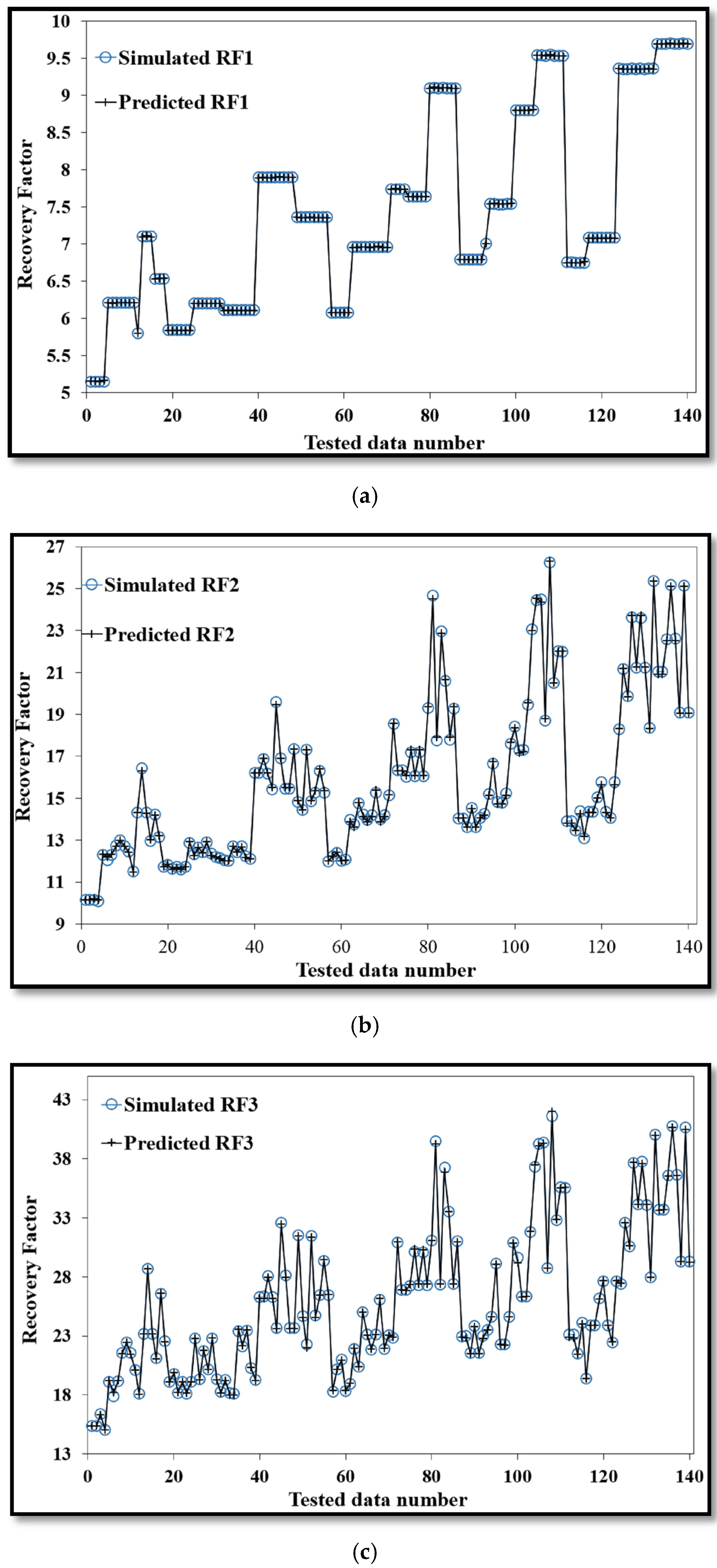
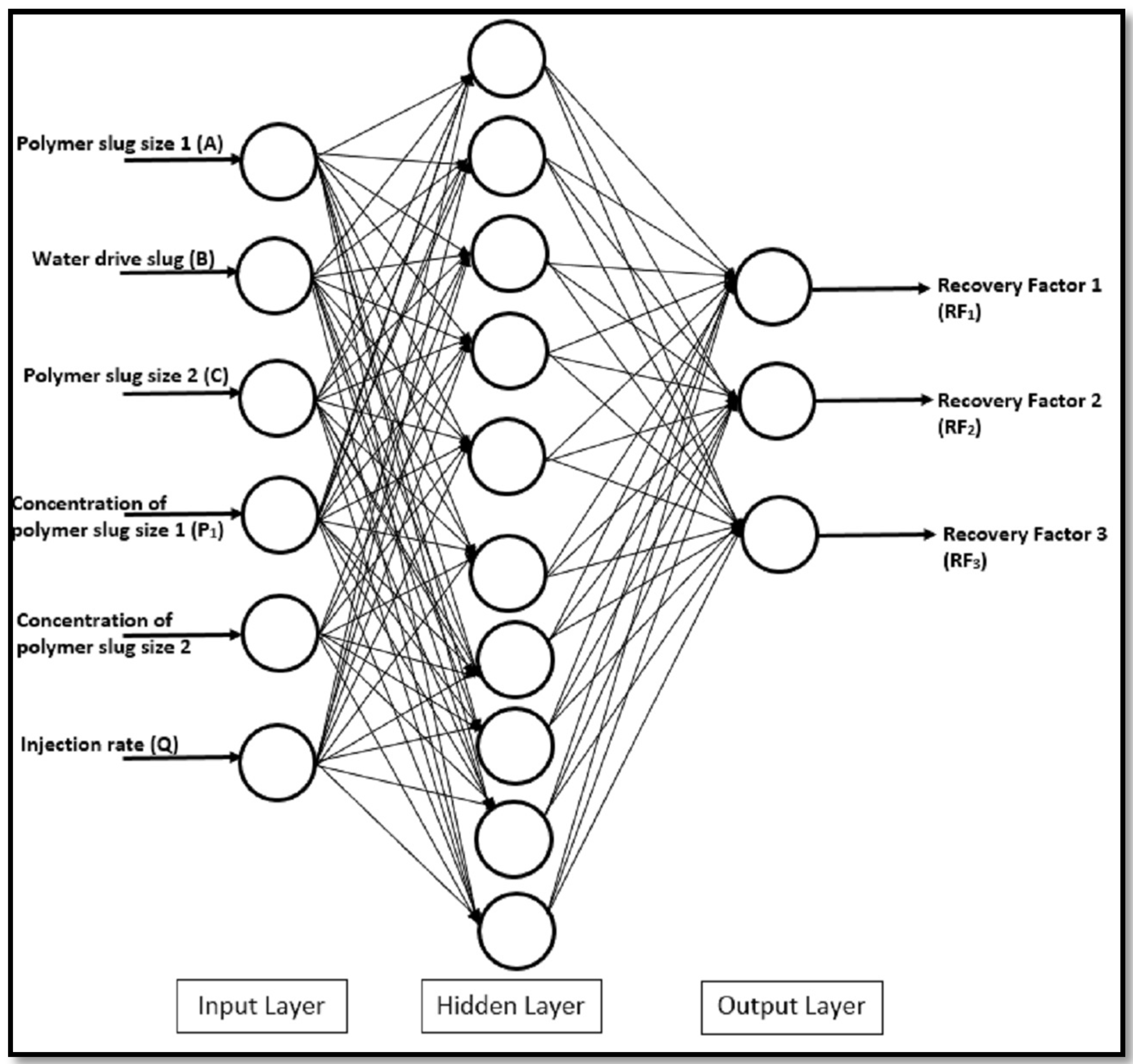
In this study, we predicted the recovery factor (RF) during polymer flooding using a neural network at three different periods: after waterflooding (RF1), after the injection of the first polymer slug (RF2), and after the injection of the second polymer slug (RF3). The results of this study can serve as an example to show the capacity of an ANN in predicting the performance of the injection of two or more polymer slugs during polymer flooding. Furthermore, a sensitivity analysis can be applied to the input parameters for finding the best-performing parameters to maximize the recovery factor.
3. Results and Discussion
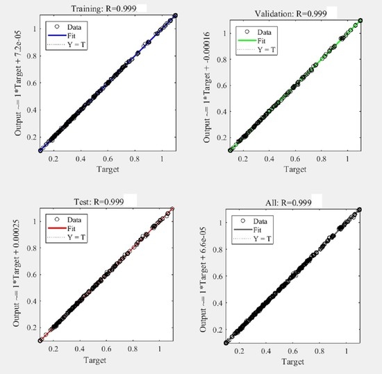
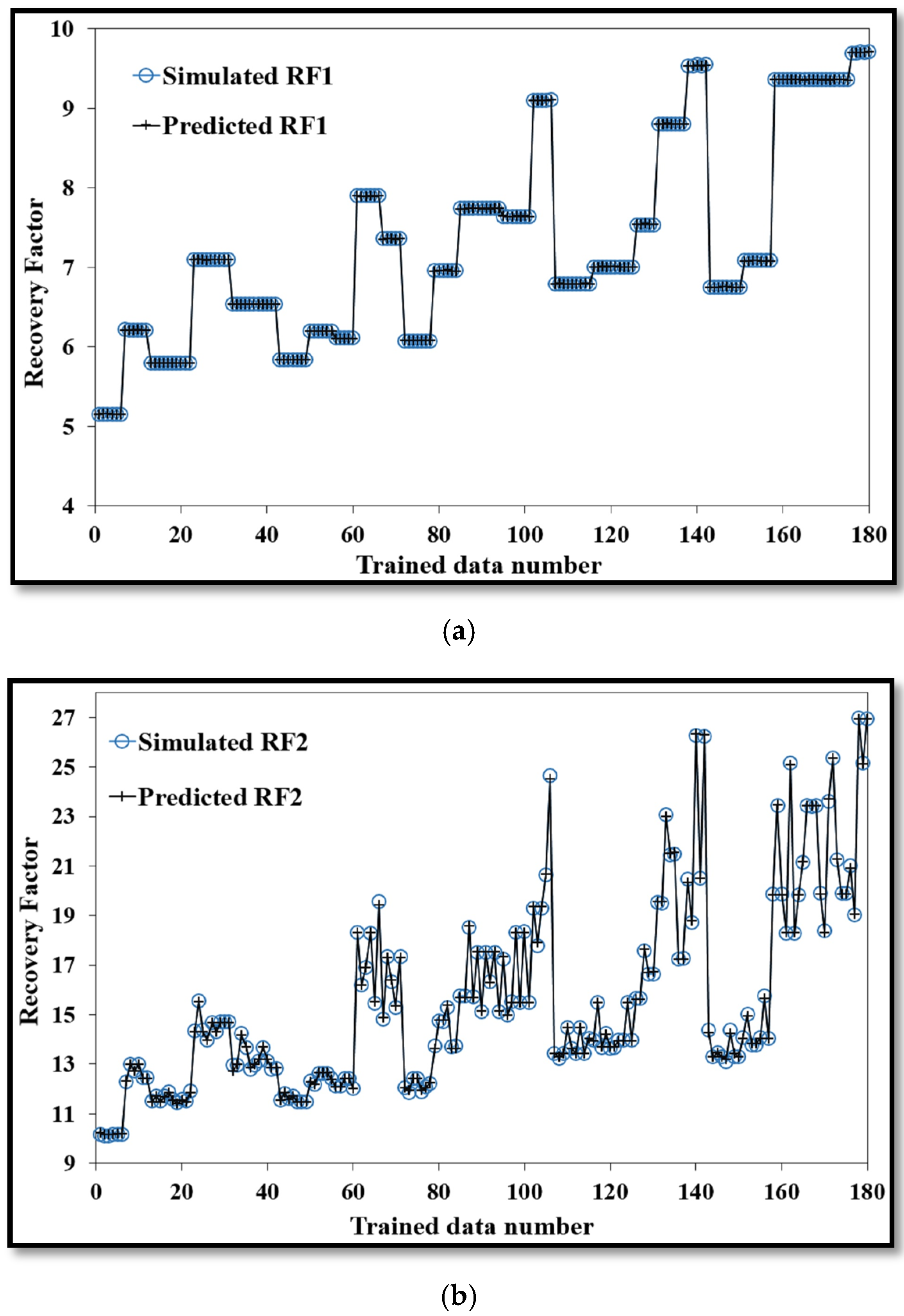
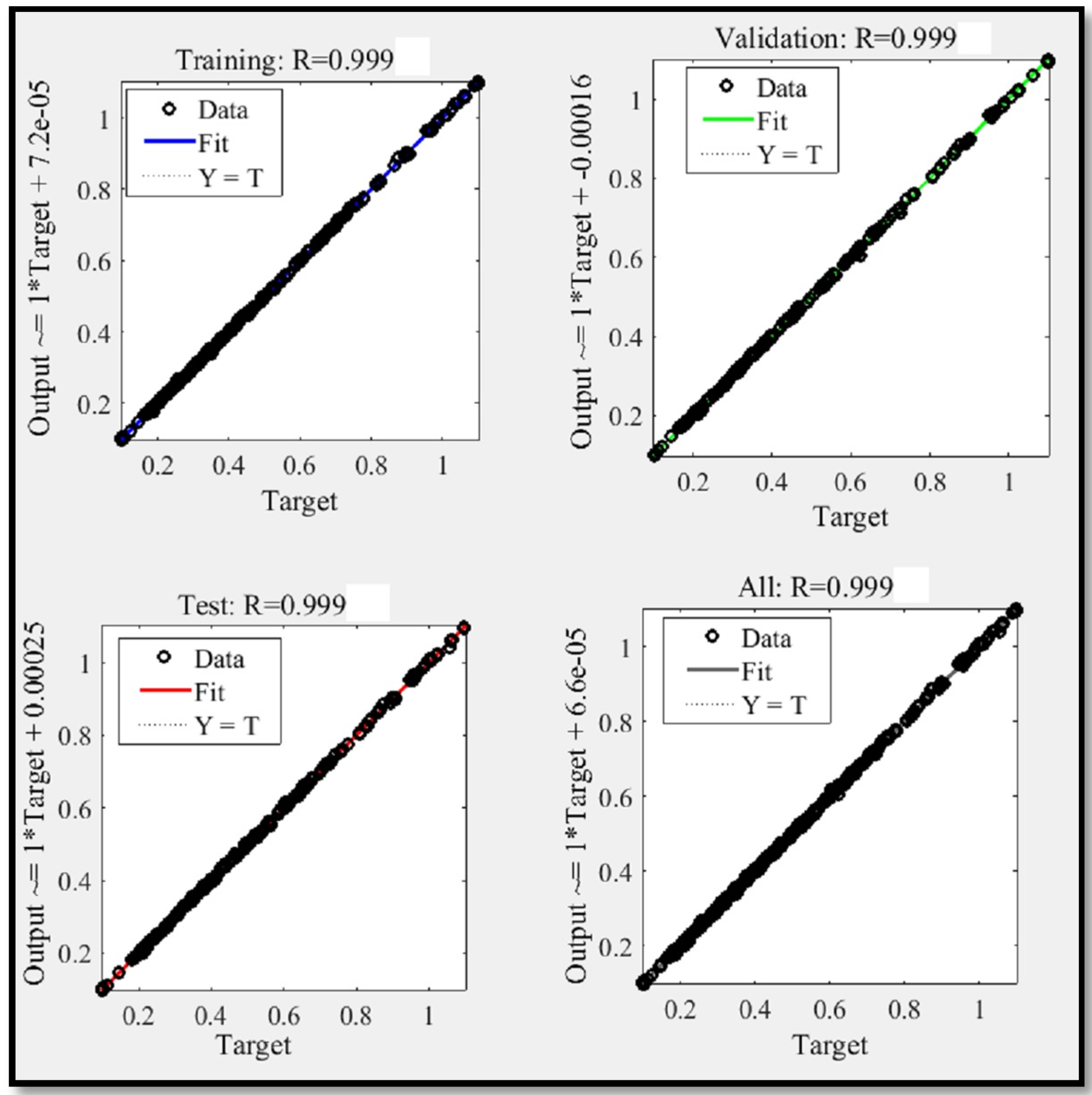
The simulated recovery factor data obtained from STARS were used to develop the neural network model. In total, 400 data points were used for this process, and these were divided into three distinct categories based on the ratios 45:20:35. The Levenberg–Marquardt back-propagation algorithm function (trainlm) was used for training the proposed network to generate a network that had the capability to generalize accurately and perform a prediction with approximately no errors.
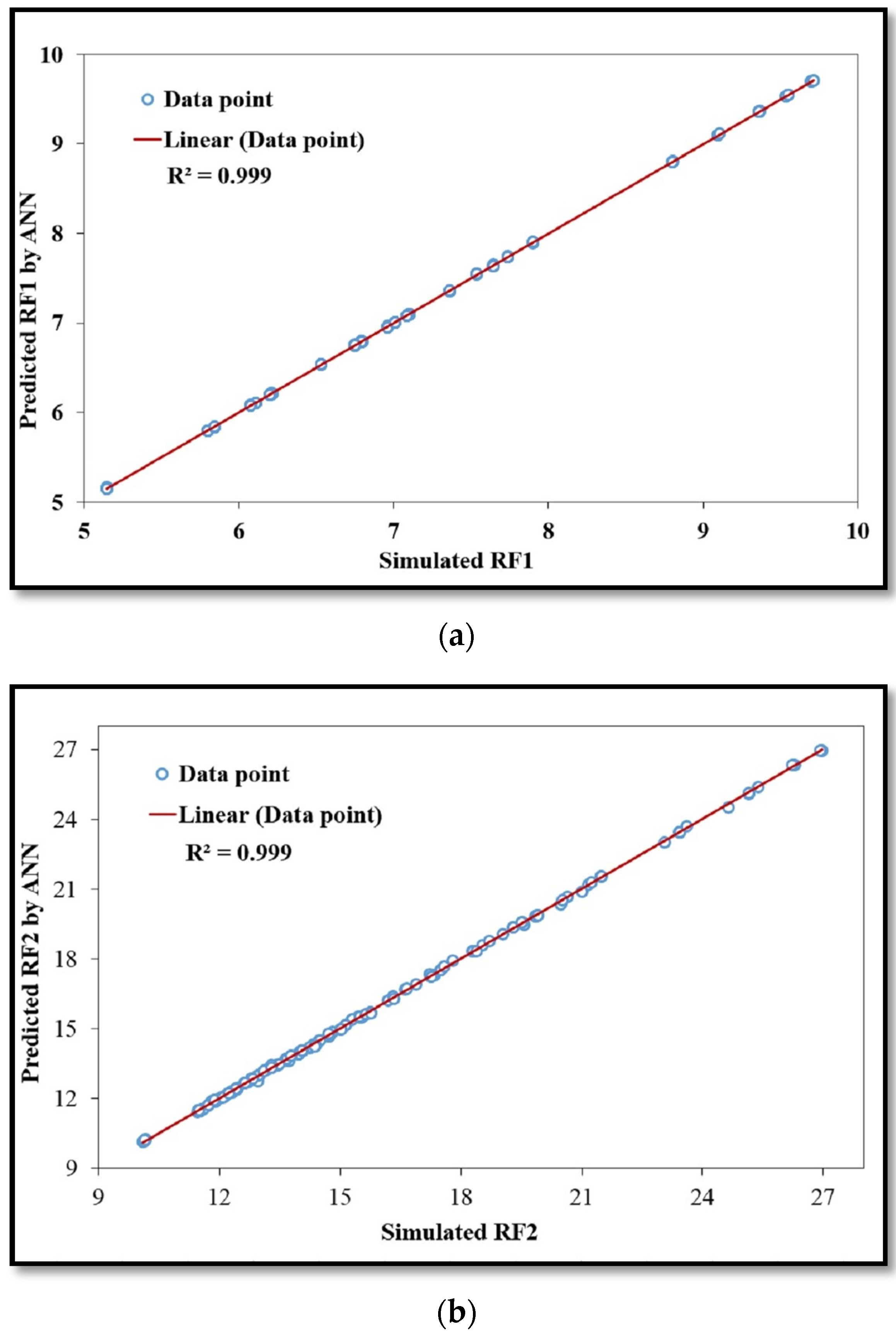
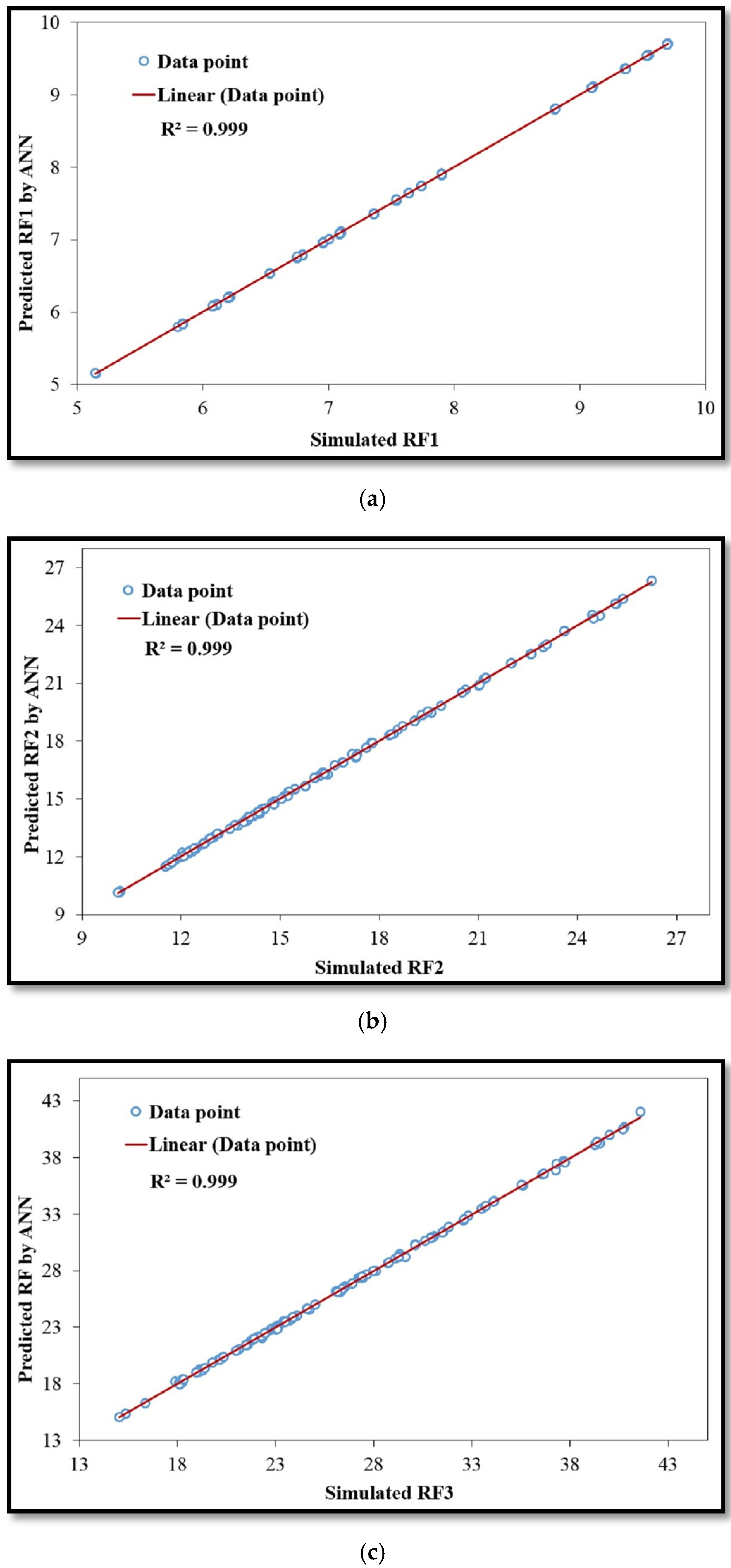
Figure 4 shows the simulated data against the predicted data obtained during the training process by the ANN for RF
1, RF
2, and RF
3. It illustrates an almost perfect linear fit. This assumption was confirmed by a correlation coefficient with an overall value of 0.999 for the recovery factor.
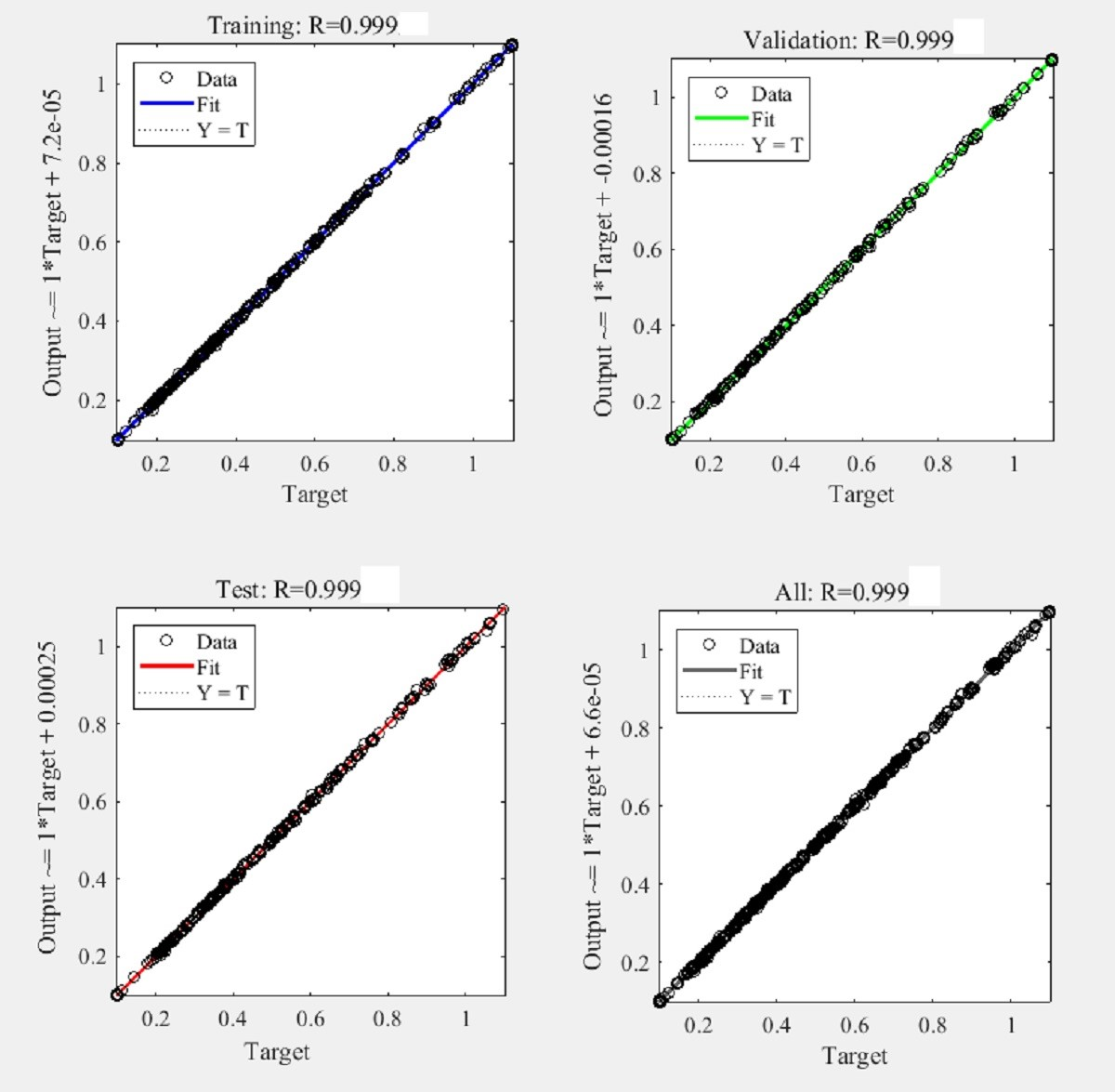
The strong correlation between the simulated and predicted data is shown in
Figure 5.
To train the ANN model, the Levenberg–Marquardt back-propagation algorithm was associated with the 10 neurons in the hidden layer. This combination led to a good prediction, giving an RMSE value of <1% (0.31%) during the validation test. In addition, the results obtained from validating the data confirmed what was learned in the training process. The R
2 values governing the output prediction obtained during the validation of the trained model were 0.999.
Figure A1,
Figure A2,
Figure A3 and
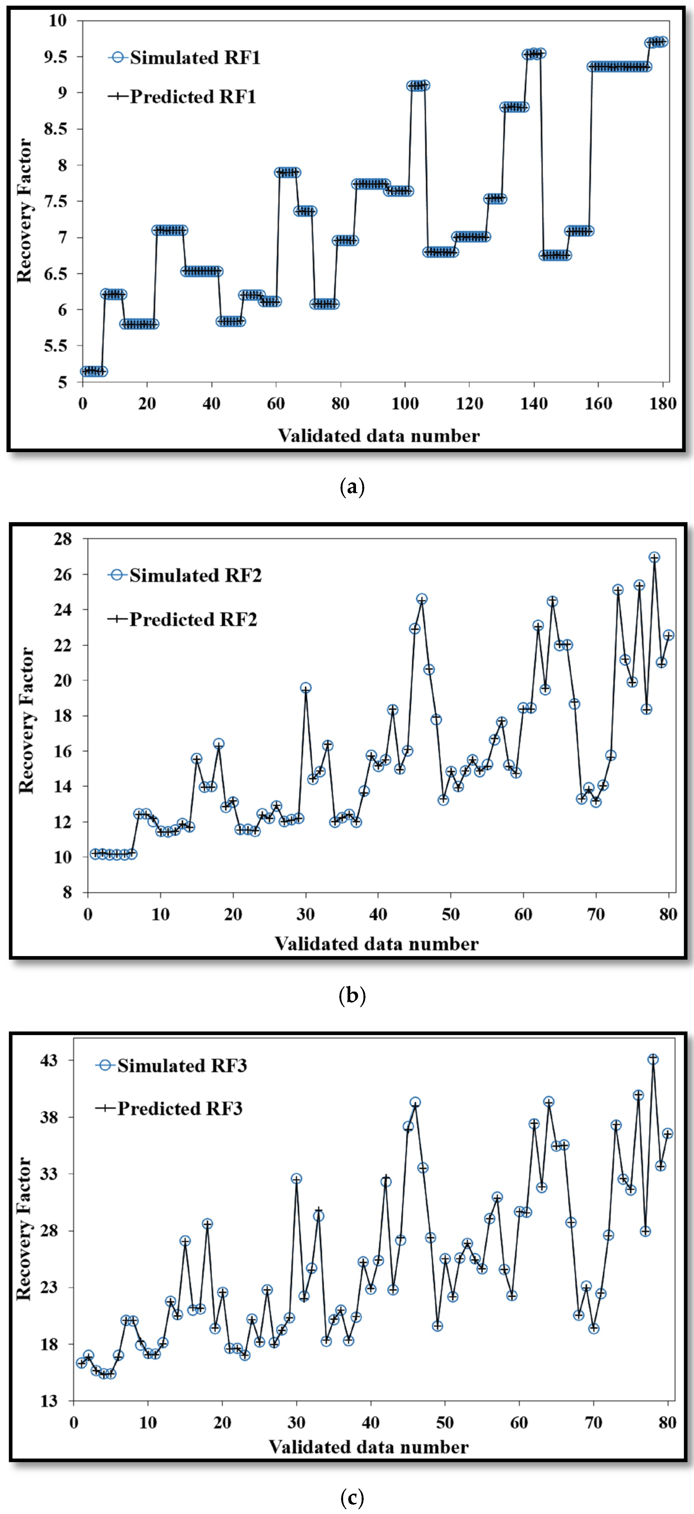
Figure A4 illustrate the simulated data against the predicted data for the validating and testing process along with a graphical representation of the correlation.
Table 5 lists a comparison of the validating results of RF
1, RF
2, and RF
3 obtained from the ANN model with multiple linear regression (MLR).
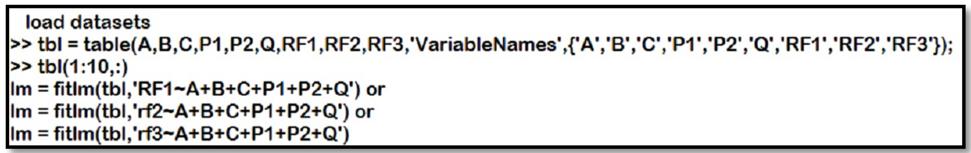
Comparing the results with other methods was very important for examining the reliability of our modeled ANN predictions against those obtained from smooth techniques before testing the whole model. Multiple linear regression (MLR) was chosen to compare the results obtained using ANN because unlike ANN, which has prediction calculations based on the nonlinearity of variables, MLR uses a linear relationship between input variables and objectives. The determination of the results of R
2 and RMSE was made possible by using the function denoted in
Figure 6 under the MATLAB environment.
It was clearly be discerned that R2 and RMSE are different. The prediction results obtained from MLR for RF1 were exceptional, demonstrating great accuracy for the prediction model. Although the result of the correlation obtained from MLR for RF1 was expectations with R2 = 0.993 and RMSE = 2.37%, while the ANN R2 and RMSE for RF1 were 0.999 and 0.11%, respectively, the ANN model still obtained better results for RF2 and RF3 (0.999 and 0.999, respectively) compared to MLR. This was also supported by the RMSE results. The MLR model gave RMSE results for RF2 and RF3 that were higher than those of the ANN (6.24% and 4.58%, respectively), but they were not better because they are not as close to zero as the model resulting from the ANN. Therefore, the prediction made by using the ANN was more precise.
Based on these results, we conclude that the predicted data precisely followed the simulated data with almost perfect accuracy. The same architecture applied for the validating process was extended to the testing process. The R2 value of the parameters was 0.999.
Table 6 presents R
2 and RMSE values for the different processes, including the overall dataset, while
Figure 7 illustrates the correlation for the overall processes.
Although the ANN model had never been used on the validation and testing dataset, it was able to give precise and accurate prediction for the recovery factor. Thus, the dataset used during the training step was new. During the validation and testing processes, the errors were <1%. It was more than acceptable to have such an error range to authenticate the capability of the ANN for modeling two-slug polymer flooding.
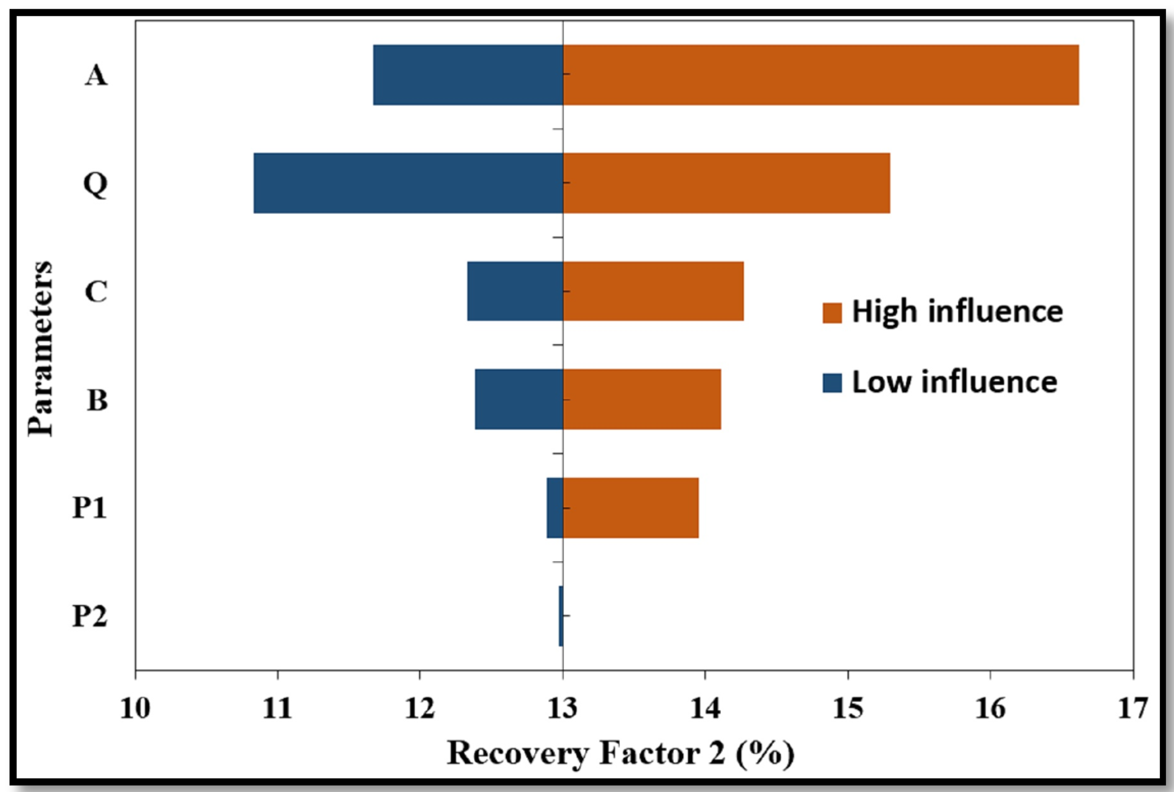
A sensitivity analysis to determine the most significant parameters influencing the two-slug polymer flooding was performed on the input parameters. This analysis was conducted in two steps, first by taking only a single parameter into consideration, and then by taking two parameters into consideration.
In the first set, there were six factors investigated for RF
2 and RF
3, as depicted in the Pareto chart (
Figure 8).
For RF
2, the chart clearly indicates that the polymer slug 1 size (A) and the injection rate (Q) made important contributions to the fluctuation of RF
2, with a contribution of >15%, while the remaining four parameters were below that range. Polymer slug size 2 (C), the water drive (B), and the concentration of polymer slug size 1 (P
1) showed poor performances. The concentration of polymer slug size 2 (P
2), however, made no significant contribution to RF
2, which could be explained by the fact that RF
2 corresponded to the period of applicability of the first polymer concentration while P
2 represented the concentration of the second polymer. Based on that, the interaction effects of AQ versus RF
2, and AP
1 versus RF
2 were investigated, even though P
1’s contribution was judged to be poor.
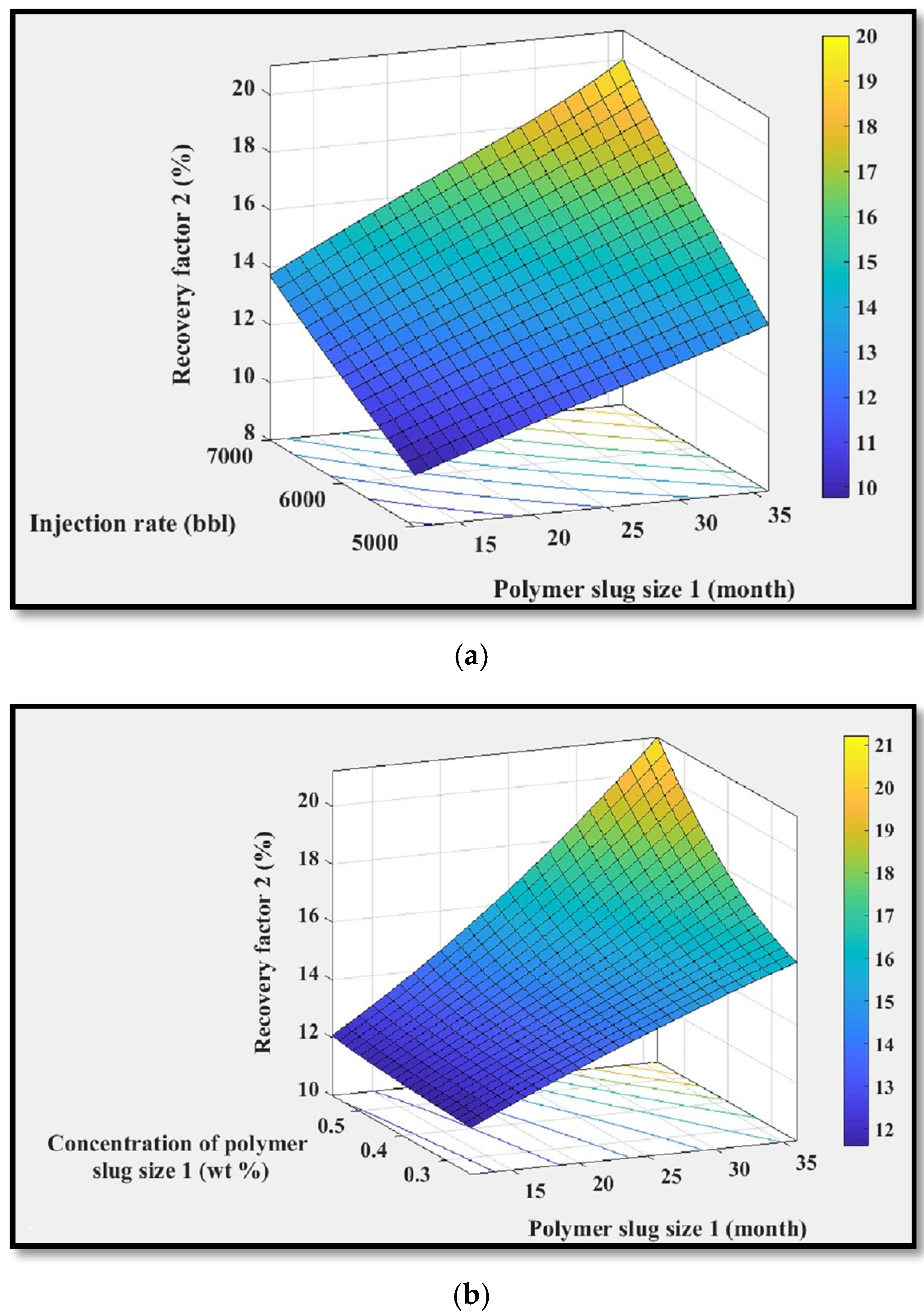
Figure 9a shows the interaction between polymer slug 1 size and injection rate. As can be seen, larger polymer slugs and higher injection rates yielded better recovery factors. In addition, even though it was not directly noticeable, the injection rate played a key role in the amelioration of final recovery. The interaction between A and P
1 was also investigated, as depicted in
Figure 9b. For periods of <20 months, the figure showed that the interaction was not effective, but starting when the slug size was >20 months, a good recovery factor was reached when both parameters were at their maxima. This clearly indicates that the effectiveness of the polymer concentration is linked with the size of the slug. A small slug size would bring poor results, even with effective design of the polymer concentration.
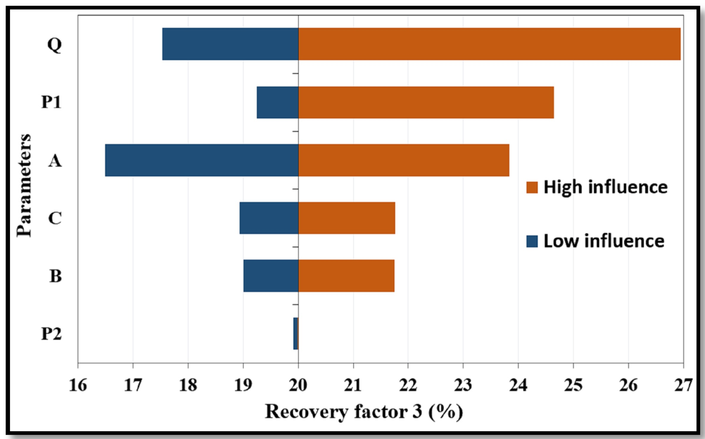
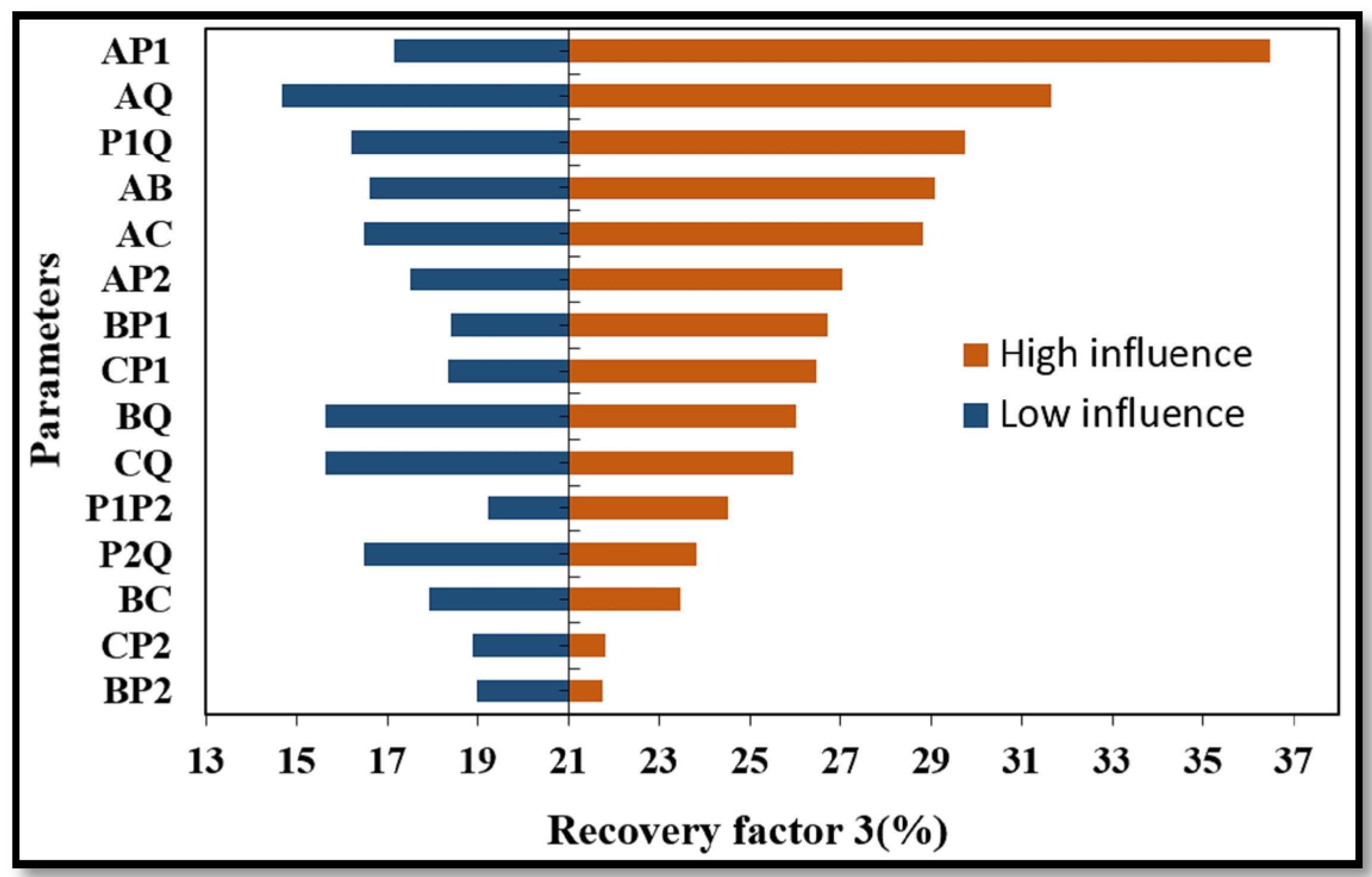
A summary of the Pareto chart showing the significance of parameters on RF
3 is depicted in
Figure 10.
Primarily, attention was given to parameters showing a contribution of >23%. Among these, Q, P
1, and A were judged in order of significance to fulfill this criterion. P
2 in this case did perform poorly while C and B gave good results, but this was below the limitation range. The poor performance of P
2 can be linked to the reduction of permeability after the injection of P
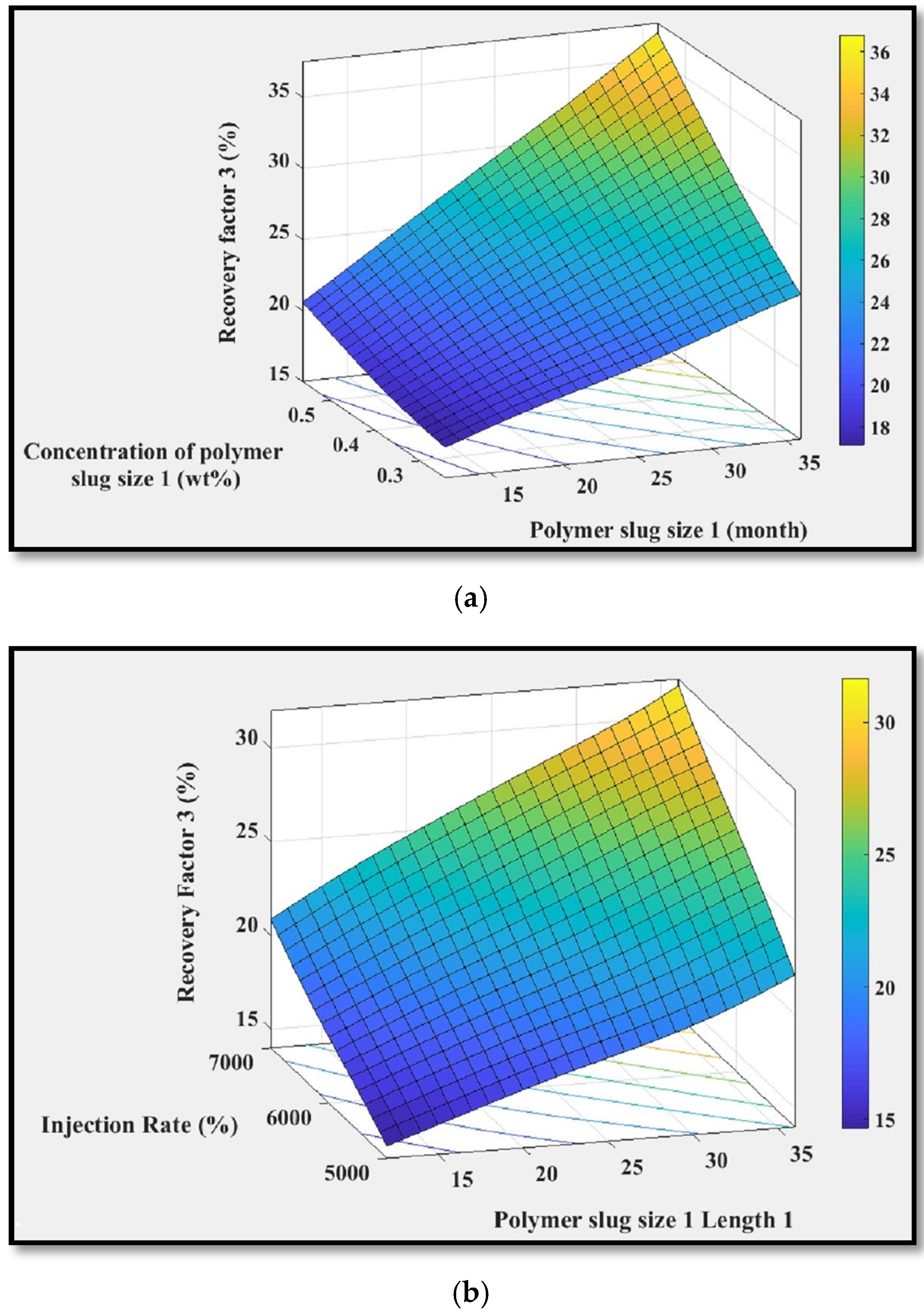
1. Basically, injecting polymer to recover more oil changed the permeability of the reservoir. If the concentration of the injected polymer is high, the permeability of the reservoir will be reduced, lowering the efficiency of a second polymer if it would be injected. To tackle this, a slightly high polymer viscosity compared to the oil’s viscosity should be chosen for the first polymer slug to allow the second polymer slug to also be effective. Plots of AP
1 versus RF
3 and AQ versus RF
3 (
Figure 11) showed appreciable rises in recovery factor (>30%), indicating a strong interaction between these parameters.
Other parameters supposed to influence RF
3 were C and P
2. It was noticeable that their contributions to RF
3 were >26%. Coupling AC showed that, to lead to better results, both slugs 1 and 2 must either be injected for a longer period or, if C is not large, A must be large, or vice versa. CP
1, however, showed a contribution of up to 26% and a good interaction between C and P
1, showing significant changes when the parameters were higher.
Figure 12 shows a summary of the coupled parameter results.
The parameters highlighted during the sensitivity analysis can then be optimized to lead to better results than those obtained during this study to minimize costs if the net present value is considered.
4. Conclusions
A simulation study and artificial neural network modeling of polymer flooding composed of two polymers slugs were performed to predict the recovery factor at three distinct periods (RF1, RF2, and RF3) in which the input data were polymer slug size 1 (A), water drive (B), polymer slug size 2 (C), concentration of polymer slug size 1 (P1), concentration of polymer slug size 2 (P2), and injection rate (Q). The modeling of the ANN algorithm was divided into three processes—training, validating, and testing—with data allocated to each in the ratios of 45:20:35. To reach accurate results, the data were normalized to be in the same range between 0.1 and 1.1. The overall correlations for the training, validating, and testing processes between the simulated results and the ANN predictions were 0.999. RMSE values were also reported to be 0.11%, 0.37%, and 0.36% for the recovery factor at the three distinct times. During the validation process, the results obtained from the ANN model were compared to those from MLR. This comparison showed that the ANN had better performance, and this was confirmed by test results in which the prediction followed with high accuracy compared to the simulated results. To conclude, a sensitivity analysis was completed to gain a better understanding of the parameters influencing the recovery factor. A first sensitivity analysis was conducted on single parameters and another analysis on coupled parameters. The results clearly showed that the injection rate and concentration of polymer slug size 1 and polymer slug size 2, and water drive size were the most significant parameters. However, the concentration of polymer slug size 2 did not play a key role in this process. This was confirmed in the MLR prediction, showing a p value >0.005. However, polymer slug size 2 had a major impact in the final recovery factor. The sensitivity study on coupled parameters showed that the coupled parameters with the most influence were in the following order of importance: AP1, AQ, P1Q, AB, AC, AP2, BP2, and CP1. Other coupled parameters not present in this list showed a final recovery factory of <26%. This study showed the capability of the proposed ANN model for predicting the recovery factor in polymer flooding with two polymers slugs with good accuracy.


