1. Introduction
Fuel consumption, in terms of economical reliability, is one of the biggest challenges for transport companies. The fact that road transport is one of the most polluting sectors in terms of greenhouse effect gas emissions [
1] has led to a resolution by the Conference of the Parties to reduce Global Warming. This resolution motivates the countries to minimize emissions. Accordingly, transport companies are forced to apply certain measures to reduce costs such as fleet renovation, changing from conventional fuel to bio-fuel [
2], preventive and predictive maintenance or efficient driving training for their drivers, the last being the cheapest way to obtain early results.
Many methods lead to efficient driving, depending on the final application of the learned techniques. In the particular case of urban public transport companies, the most common method consists of an initial training day, including one practical individual session. In that session, each driver drives a route and the trainer observes his or her mistakes and strengths. After that, all drivers attend a theoretical session in which the national or international recommendations on efficient driving are explained [
3]. Finally, in another practical individual session, the drivers apply the learned techniques following the indications of the trainers. Monitoring the vehicles and allowing trainers to check the evolution of the performance of the drivers and to prepare periodic reinforcement sessions based on a more objective evaluation may complete this initial training day.
Regarding the evaluation of the driver’s performance, there is more uniformity. Most companies check the evolution of consumption as the evaluation metric. Nevertheless, it has been shown that this is not a good way to assess the driver’s performance, as fuel consumption depends on too many aspects that are beyond the control of the driver such as the weather or the density of traffic and not only on his or her driving skills [
4].
Our process dismisses fuel consumption as an evaluation method. Thus, in our previous research we developed an evaluation method based on some efficient driving patterns [
5]. This method allows us to perform an objective evaluation of the skills of the drivers because it is based on real driving data. Furthermore, it is also able to facilitate adaptive training as we can see the evolution of the performance of the driver in each pattern and focus the reinforcement sessions on his or her mistakes [
6]. All the real data of our studies are obtained by a system called Cated Box, which receives information directly from the vehicle’s engine control unit (ECU) [
7]. This is already under application in 16 professional fleets in Spain and Morocco, involving 880 professional drivers.
In the way that our system obtains the data, it is impossible to know why a driver behaves in a particular way. Nevertheless, observation of data and experience allow us to make assumptions. Our training method promotes safe and efficient driving. That includes anticipation, and keeping the safety distance is paramount to anticipation as it minimizes the influence of other vehicles on the performance of a driver. Thus, every driver, no matter the density of the traffic, must strive to maximize the use of inertia.
In this paper, our main goal is to show the economic impact, in the form of money saving, that the application of some of the efficient driving recommendations may generate in an urban public transport company. To do so, we analyze real driving data gathered from one single vehicle during a complete month. This means analyzing a total amount of over one million samples. We compare a real track in which the driver decelerates in an inefficient way with an ideal theoretical track obtained from the linear regression. This ideal track simulates a perfect inertia deceleration with null consumption. The real track is conformed by data gathered during the normal activity of the vehicle. As we explain in [
8], these data are sent to the central system and processed in a learning analytics module. In this case, we represent an example of real driving in terms of speed and distance.
The paper is structured as follows; in
Section 2, we make a review of related work.
Section 3 gives a background to the study while
Section 4 shows the methodology applied for the calculations.
Section 5 gives the results of a brief case study, and
Section 6 includes the discussion and conclusions.
2. Related Work
There is ample literature on the influence of efficient driving on fuel consumption. A good overview can be found in [
9] as it shows the methodology, type of study, and results for the most relevant studies made in recent years.
Different types of techniques are applied in the literature to quantify the problem of fuel consumption. In field tests, the authors usually apply their own methodology to actual vehicles and drivers and obtain results that are real or, at least, estimated from real data. The dimension of the experiments in the overviewed literature varies from three drivers performing a training route of 15 km [
10] to 54 drivers who perform routes of 16 km over a period of six weeks [
11]. All these studies show that the application of efficient driving techniques increases savings in fuel consumption. However, these studies are focused on a set of basic recommendations on efficient driving with the aim of reducing fuel consumption. Our approach is different as we use efficient driving patterns as the basis of an efficient driving learning methodology, the main goal of which is the modification of driving habits of professional drivers to perform more efficient and safe driving, but it also allows noteworthy fuel savings. These patterns have the particularity of having a temporal dimension instead of being a combination, simple or complex, of instantaneous events. Therefore, we base the potential fuel savings on the application of an efficient driving pattern, inertia, that describes the driver’s behavior in a temporal window. In addition, our dataset is composed by real data, obtained during the complete working day activity of the professional drivers, while other related works are constrained to prepared scenarios. In this sense, the work presented in [
12] also highlights that drivers should be evaluated during their normal work activity because fuel saving goals could be affected by other external factors. Furthermore, the deceleration during inertia is the result of a linear regression model, which is also a novelty.
Nevertheless, the range of fuel saving varies between the 1% obtained in highway testing with the help of a real time on-board assistance device [
13] and the 18.7% obtained in 1 km long sections with three intersections [
14].
The authors in [
15] compare two different approaches in two public transport companies. It is very relevant to our research as they obtain data from an on-board device from vehicles and drivers during their professional activity. One of them provides data to illustrate in-class regular training and the other sends real-time alerts. Both systems use isolated undesired events such as excessive speed or prolonged idle time to advise the drivers on their behavior. Our pattern method is not attached to single-instant events but is opened in a temporal window, which provides a wider overview of behavior and context.
There are also some review papers or reports by organizations in which the authors give their conclusions based on the material available that fits their requirements. Of these papers, [
4] provides the greatest improvement in consumption (up to 30%) by comparing efficient and aggressive driving and using a speed control device. The lowest savings are shown in [
16], ranging from 5% after training to 15%, depending on the driver. The authors ensure 10% if a real time assistance device is used.
Finally, a last type of paper is that in which the authors develop a mathematical model that seeks to calculate the benefits of efficient driving. Although not comparable as they use different metrics, in [
17] the authors achieve maximum savings of 34% with an algorithm tested under standard urban traffic. Additionally, [
18] obtained a saving of 1.5 l/100 km with an algorithm based on micro-economic theory. They performed tests in five stages, considering different levels of density and traffic accidents. For a mixed consumption of 10.24 l/100 km, their results achieve savings of 14.6%.
To our knowledge, there are no references in the literature in which inertia is used in the same way as in our work. We apply a linear regression model based on real driving data in order to obtain an ideal deceleration without fuel consumption by using inertia as an efficient driving technique. Then we compare this ideal function with real data using the brakes to see the differences in fuel consumption. Starting at the same point and speed, a vehicle using the brakes will only reach the same point and the same speed as another using inertia if the former accelerates during a certain period of time. We calculate the cost of using the brakes by checking the consumption caused by that acceleration in contrast with the null expense of fuel required by inertia driving. It is an effort to quantify the impact of anticipation separately from the other efficient driving techniques.
3. Background
The present study is based on the theoretical good usage of inertia when a vehicle is approaching a stopping point or when speed needs to be adapted to slow traffic ahead. It has much to do with the anticipation of traffic and service situations.
We initially developed the inertia pattern [
5], in which we looked for periods of time in which the vehicle was in motion and gear engaged without consumption. Its key performance indicator (KPI) is the percentage of time in which the vehicle runs with no consumption. This was a first approach to inertia as an efficient driving pattern. At that time, we could only obtain certain parameters from the vehicle to define inertia. The use of the brakes was not included among those parameters, although it is a key element to determine the way inertia is conformed.
With an extension in the amount of data registered by the system, we started to obtain the parameter of the use of the brakes by the driver, and thus we saw the chance to study how that initial inertia pattern was conformed. Thus, we developed a set of complex inertia patterns that improve our detailed knowledge of driving conditions. The definition of these patterns follows.
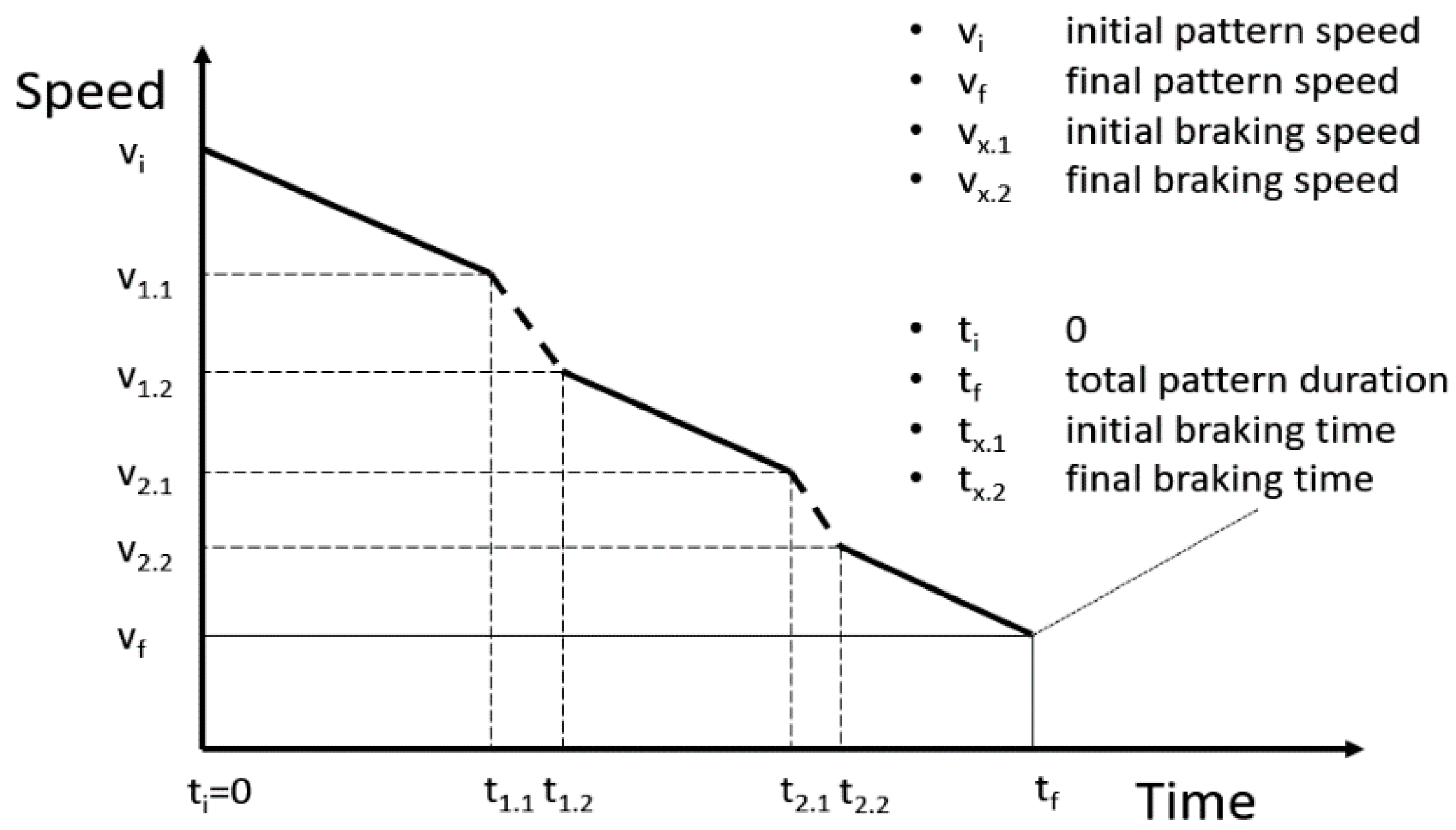
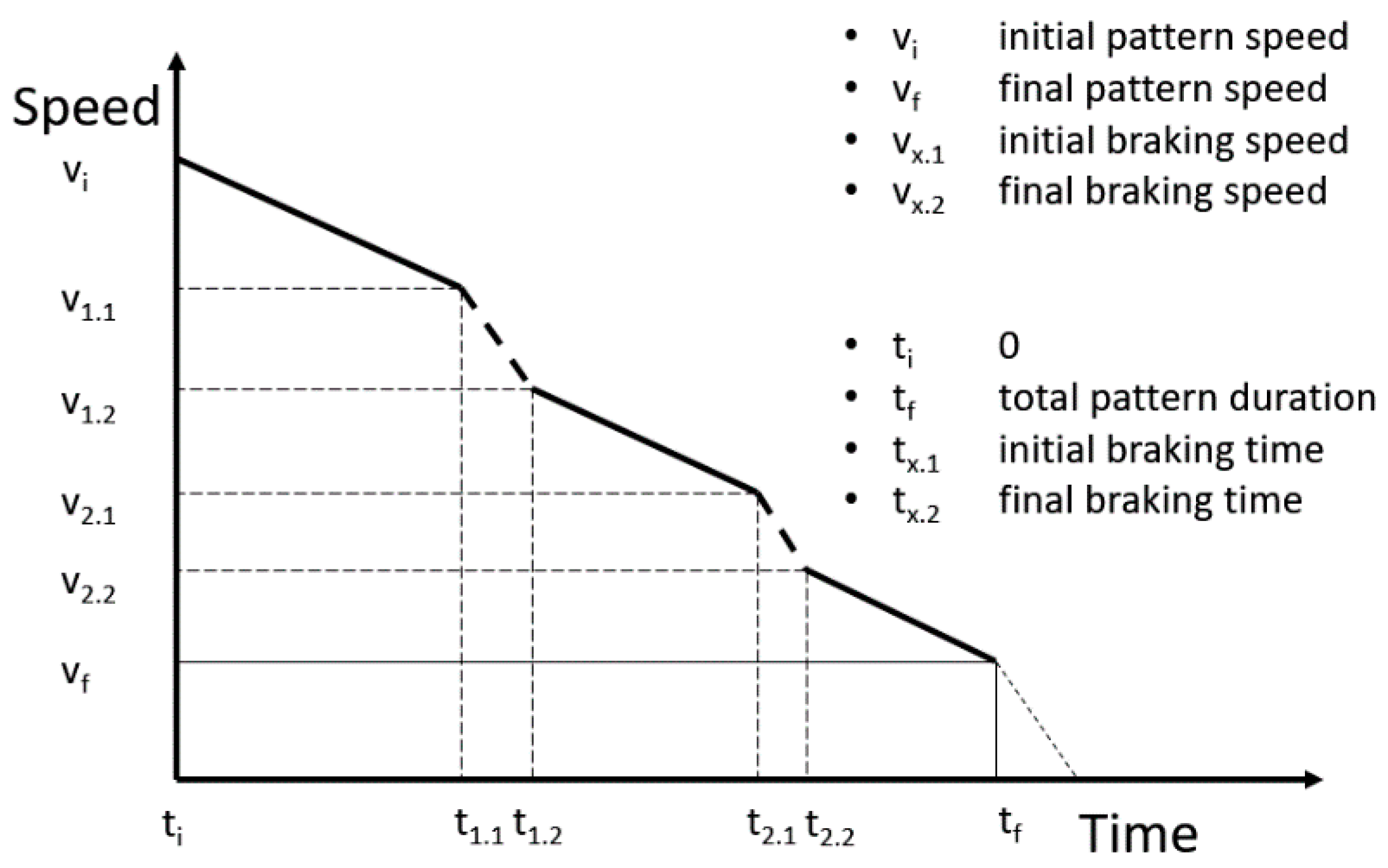
3.1. Pattern of Corrected Inertia without Stop (#1)
The driver starts decelerating in inertia and corrects the speed with the brakes so that stopping is not finally necessary, as
Figure 1 shows. It may appear next to a traffic light that is initially red that becomes green before the vehicle arrives at the stopping point. The continuous lines show the periods in which inertia is used, and the dashed lines show those in which the driver uses the brakes. The
parameters show the relevant speed values along the pattern such as the initial speed (
), braking start (
), or the speed at which the driver retains inertia (
).
represents the final speed of the pattern and the point at which the driver accelerates again.
We can ascertain the total loss of speed of the pattern just by subtracting the initial speed from the final speed as follows:
In addition, we can calculate the speed loss due to the use of brakes as follows:
where
is the number of braking periods in the whole pattern and
is the order number. Finally, we can calculate the loss of speed due to inertia as follows:
The calculations to determine the time of use of the brakes and the time of inertia () are equivalent.
The KPI for this pattern is the percentage of time of use of the brakes () against the total duration of the pattern ().
The rest of the patterns have the same structure, the only difference being what happens after the pattern finishes. While in this case the vehicle does not stop (there is a long acceleration after the inertia period), the other two patterns result in the stopping of the vehicle but in different circumstances.
3.2. Pattern of Corrected Inertia Long (#2)
As we have explained previously, this pattern (
Figure 2) has the same structure as the other complex patterns of inertia but with a necessary stop at the end, which is probably a red traffic light or a bus stop.
The KPI is the percentage of time using the brakes compared with the total duration of the pattern, exactly as in the case of the first pattern.
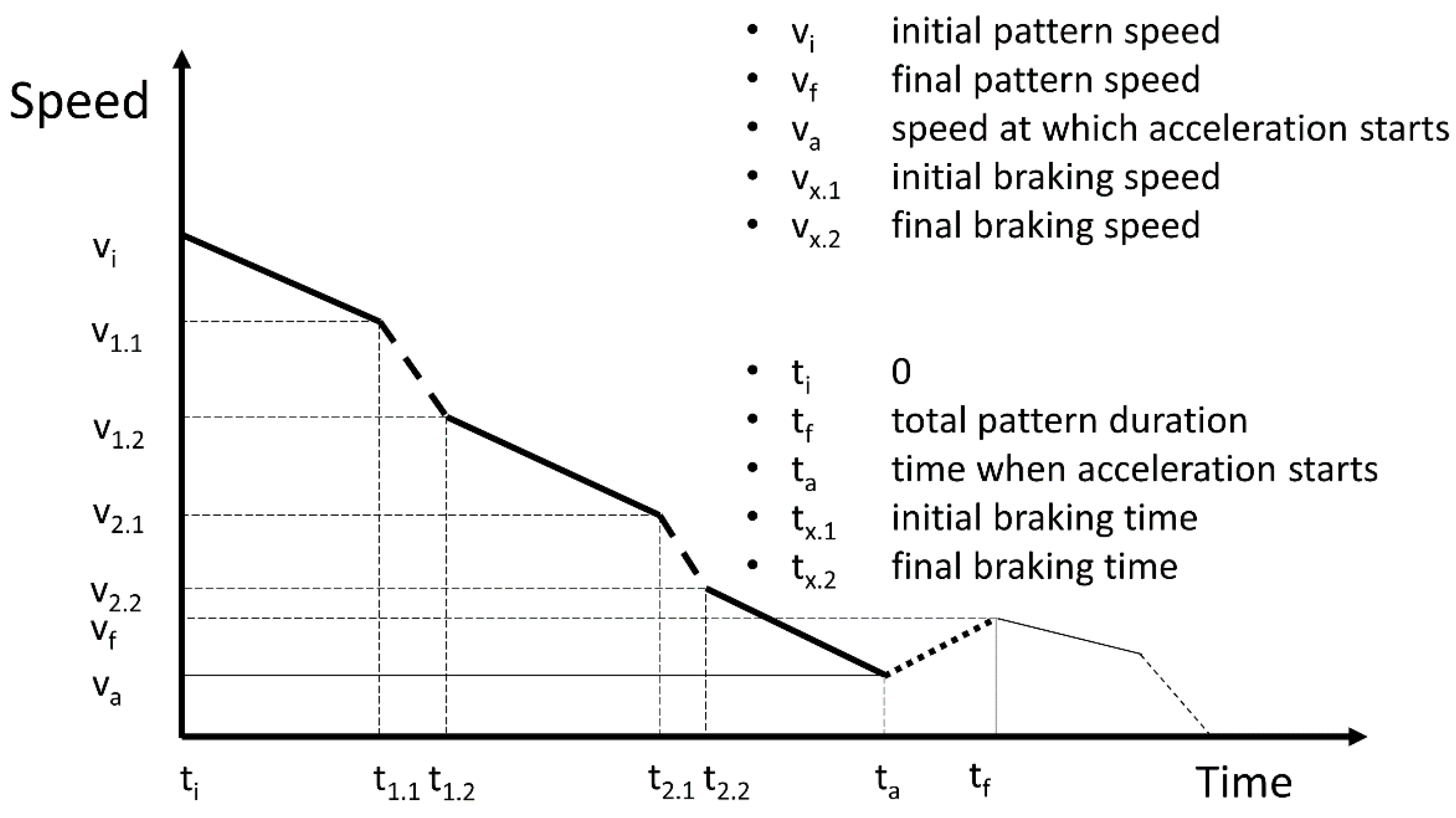
3.3. Pattern of Corrected Inertia Short (#3)
This pattern (
Figure 3) again has the same structure but with a short acceleration period at the end, represented by a line of dots, caused by a bad estimation of the driver of the distance that the vehicle is able to run with its inertia.
This pattern has two KPIs. On the one hand, we have the percentage of time of use of the brakes compared with the total deceleration time (), as in the previous patterns.
On the other hand, we have the percentage of time of the final acceleration compared with the total duration of the pattern (.
The goal of designing these patterns is to determine how drivers perform inertia. The patterns show how drivers behave in terms of performance and anticipation. It is not the same trying to stop the vehicle (patterns #2 and #3) or just trying to adapt the vehicle speed to that of the traffic (pattern #1).
4. Methodology
The objective of the methodology is to find out how much fuel is spent prior to one of our patterns from the point at which inertia could have been started to be used to arrive at the same point at the same speed. This amount of fuel is what the vehicle consumes during the acceleration.
We estimate that a month provides a sufficiently large enough set of data for the methodology to be valid. From these data, we obtain the different cases in which the patterns explained in the Background section appear and select an appropriate one for our purpose. To be more representative, the selected pattern should be as long as possible to give a wide amount of results. Furthermore, the KPI should be similar to the mean KPI of the fleet, which is registered in our records from the company. We then compare the selected pattern with an ideal one. In this ideal pattern, the driver does not use the brakes until the rpm (revolutions per minute) are close to idle. While the ideal curve only shows a long inertia period, the real one alternates inertia with the use of the brakes. Thus, an acceleration period appears in the real track curve, so the initial and final speeds and positions are the same.
To find the point in which the driver should have started to exploit the vehicle’s inertia, we develop a linear regression model based on the same real data that includes the studied track. Other modeling techniques could be useful to improve the accuracy of our predictions such as classification and regression trees, Knn (K-nearest-neighbour) Clustering, and Neural Networks. Nevertheless, in [
19] the authors explain that when working with real world situations, variables do not change independently. Thus, multivariate regression is the appropriate method since it can assess the independent effect of one variable controlled by the others.
Furthermore, stepwise linear regression removes the weakest correlated variables after considering all candidates. Authors in [
20] explain how the models resulting after using this method only include the variables that best explain the distribution of the dependent variable, according to their statistical significance (
and efficiency (increase in the
and the
above a predefined threshold).
The result of this linear regression model is theoretical instant acceleration (deceleration in this case) considering speed, engine regime, engaged gear, and use of brakes at each particular point, starting with the final one according to the real curve. This final point is identified as
in the graphical representation of the patterns shown in
Figure 1,
Figure 2 and
Figure 3. Once the acceleration value at the final point is obtained, and knowing the elapsed time for the corresponding sample, we can calculate the speed in the instant of the previous sample and thus the travelled distance. Repeating this process, we confirm the simulated track curve.
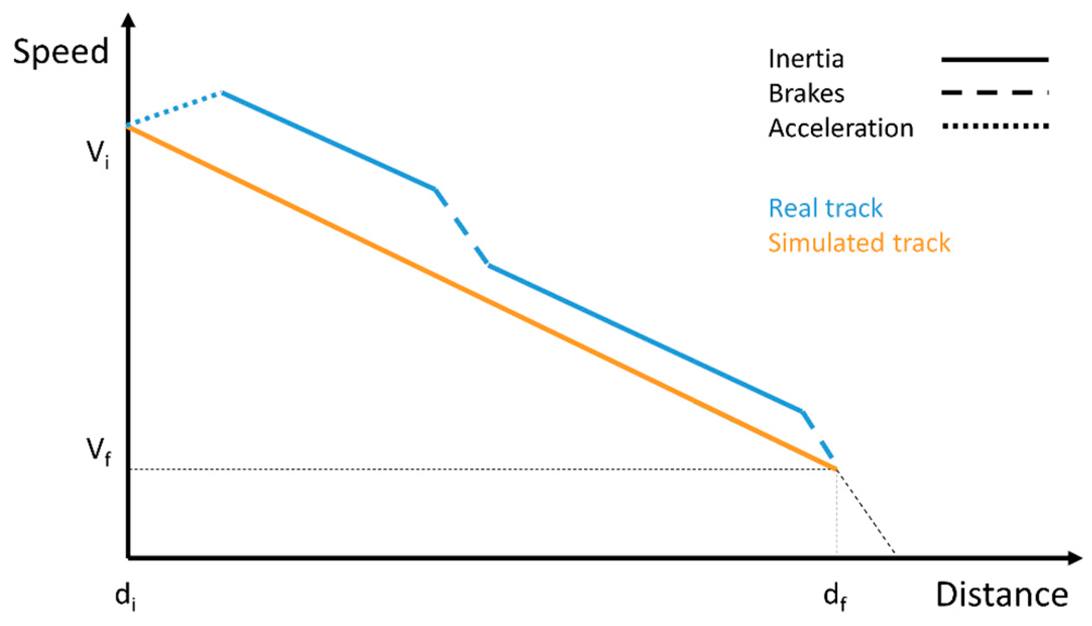
Figure 4 shows a schematic representation of the ideal and real tracks. While the ideal curve shows how deceleration would be subject to a single inertia period, the real curve, after an acceleration period, alternates inertia with the use of the brakes, which implies harder decelerations. Both curves start and end at the same point.
4.1. Data Set
For the model to be valid, we must select a large amount of real data for a single bus, regardless of the driver. The reason is that, in this case, we are not evaluating the driving skills of the driver. We only consider the difference between applying the efficient driving recommendations or not, and we want to minimise the dispersion of the vehicle’s mechanics in the results. As we only use one vehicle, we have the same response if the conditions are the same.
The data must be filtered as we are only interested in inertia; that is, data with null fuel consumption. All data were captured by the cated box system [
7]. The structure of the data is shown in
Table 1.
This makes 22 parameters that we need to filter so they become adequate to the peculiarities of our study. In this case, we are only interested in the samples showing an inertia pattern. This means that all the samples we use have:
(maximum value accepted by the system)
Therefore, the rest are not relevant in the linear model, and they can be discarded. We can also discard other parameters that are not of use in this case:
This is only an identification number and is of no use in a linear model.
We only monitor one vehicle.
The text format makes this difficult to manage. It is better to use .
The low refresh ratio makes this useless for us.
This parameter is of use in those vehicles without controller area network (CAN).
This shows the same number as the parameter with a delay of one sample.
This has the same issue as .
This has very low refresh ratio .
There is no need for geolocation.
There is no need for geolocation.
Taking all of the above into account, our final set of data will be composed by:
4.2. Linear Regression Model
The objective of this linear regression model is to determine a function that allows us to verify the deceleration of the vehicle depending on the speed, rpm, engaged gear, and the use of brakes in every single moment, and the initial expression structure is:
where:
The variables , are continuous, while , are categorical. This means that can only take exact values. In this case and . The reason why there is no term is that, in decelerations, the ECU (Engine Control Unit) always engages the first gear in idle conditions, so fuel consumption is never null.
We used MatLab (The Mathworks, Inc. Natick, MA, USA; Matlab R2015b: Statistics and Machine Learning Toolbox) to develop the linear model we have just described.
5. Case Study
We have applied our method on an 18 m long articulated bus that belongs to the municipal transport company of the city of Gijon in the north of Spain. This bus is driven by different employees of the company and always does the same route. The raw data for this case study were obtained during December 2015, and the total amount is over one million samples. The bus completed the route 611 times, considering its two directions. A first filter on the raw data gives us a full set of 174,344 samples with null consumption. This filtered set conforms the data to undertake our linear regression model.
In addition, a glance at the weather internet portal
http://www.wunderground.com shows that conditions in Gijon were very variable that month. There were 12 rainy days out of 31 and two foggy days (low visibility), and the temperature varied from a maximum of 24 °C (15 December 2015) to a minimum of 3 °C (1 December 2015). Thus, a wide range of weather conditions is covered.
The results of a first iteration are as shown in
Table 2. First we can see the function of the model and then the chart of results. The coefficients can be seen in the first column, where the
is the independent term and the categorical variables have their different values by their sides. The
column shows the estimated coefficients for the different parameters,
shows the standard error, and
. Finally, the
p-value column has values below
, meaning that the
coefficient is not valid in less than 5% of the cases. If it were higher, we would dismiss the parameter.
The second part of
Table 2 shows the statistics of the model as the Number of observations or the Error degrees of freedom.
The Root Mean Square Error estimates the standard deviation of the error distribution. The R-squared (coefficient of determination) suggests the level of explanation of the variability in the response variable. The F-statistic tests if there is a significant linear regression relationship between the response variable and the predictor variables. Finally, we have the p-value for the F-test of the model that shows if the model is significant or not.
We can see how the most influential term is the engaged gear () as the value is higher than any other parameter coefficient for all of its categorical values. The influence of the use of the brakes is also important, and the rpm, as the result of its product by the corresponding coefficient, has a similar value. On the contrary, has a lower influence on the results of the regression, although it is also relevant. shows that the is significantly higher than the standard error (SE) for all parameters, reflected in the p-value column, which is in all cases far lower than .
In accordance with the value, the variable would be very important. Obviously, the use or not of the brakes dramatically affects the value of the deceleration of the vehicle. In our study, we aim to characterize the deceleration when the driver uses the inertia of the vehicle. Thus, the does not affect the results. As the engaged gear during all the deceleration process in this case is , the other variables do not have any effect on the results.
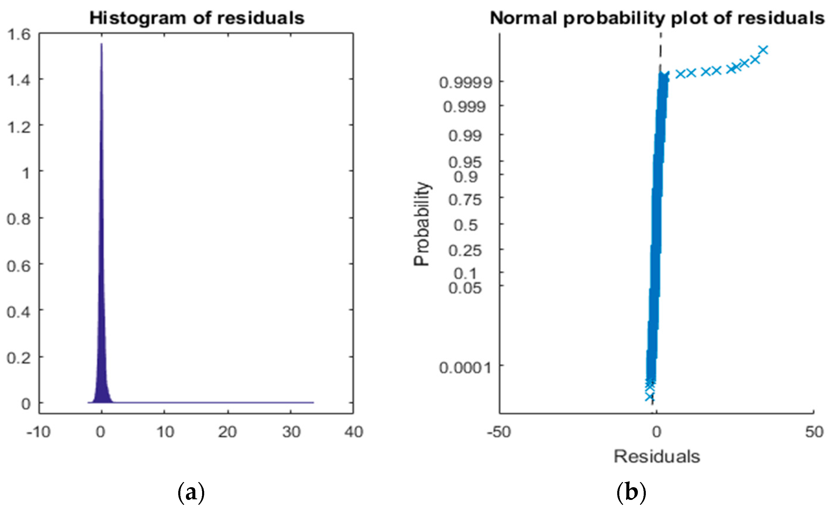
To examine more closely the results, we launched an ANOVA analysis to check the variance. Our model shows good results regarding the
p-values of the coefficients and F-tests, but the coefficient of determination
R-squared is too low, so we will try to improve it. If we display the residuals of the model as in
Figure 5, we can see how the histogram has a very long tail. This means that the distribution of observations is not normal, so we need to adapt it to make it useful. To that end, the first step is to find and eliminate the outliers.
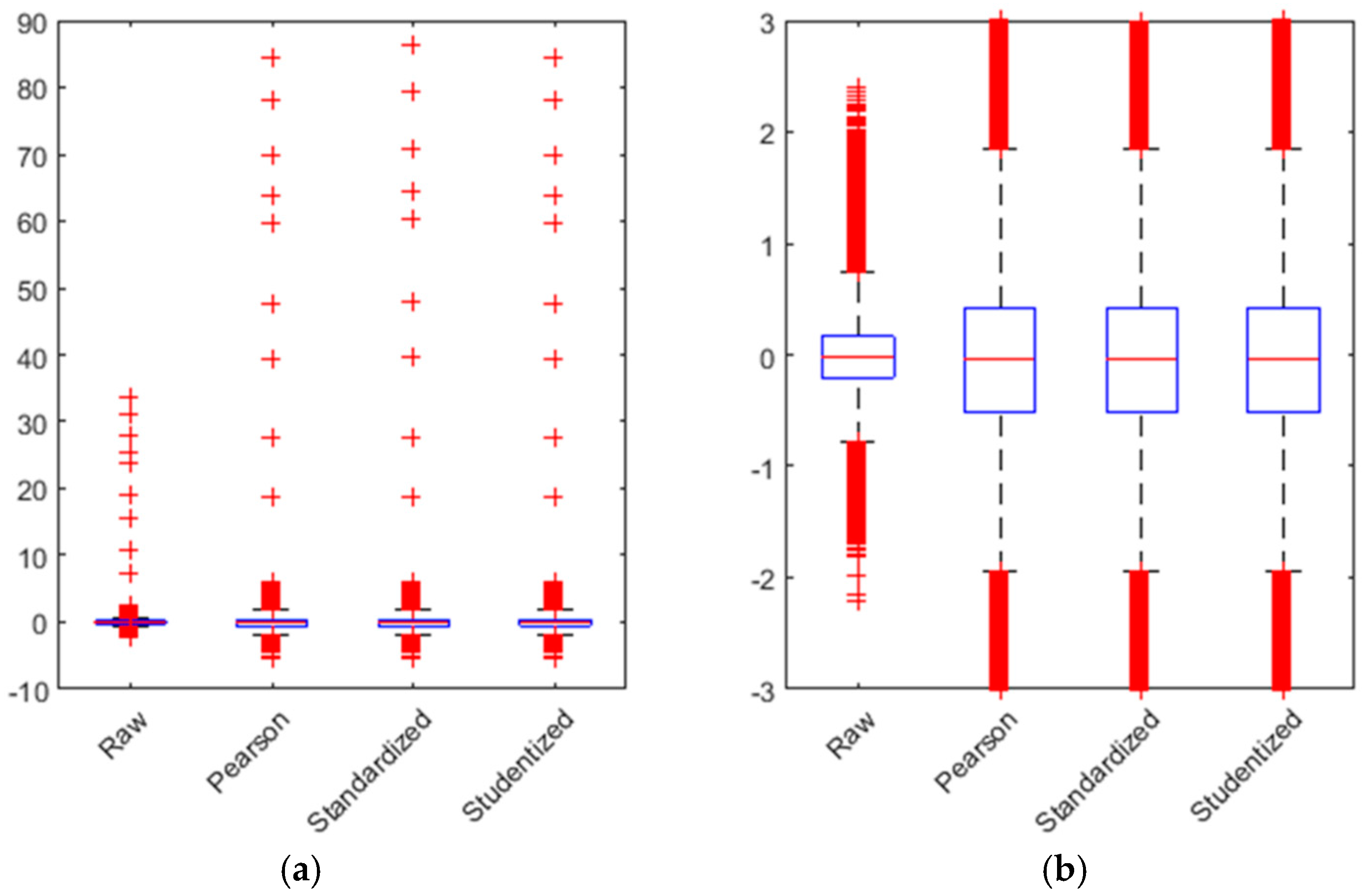
The scatter plot of residuals in the first iteration showed evidence of the existence of outliers (
Figure 6).
In the boxplot, we can see the representation of all outliers (in the left image). We have zoomed in so the values of the valid residuals can be better appreciated (
Figure 7).
All the outliers are shown in red in the figure. We use a whisker
, which is plus/minus 2.7 times the typical deviation. With this value, the outliers are defined in Equations (8) and (9).
where
is the whisker,
is 25th percentile, and
is the 75th percentile. With this approach, we eliminate 8618 outliers, which is less than 5% of the total data population, as shown in Equation (10).
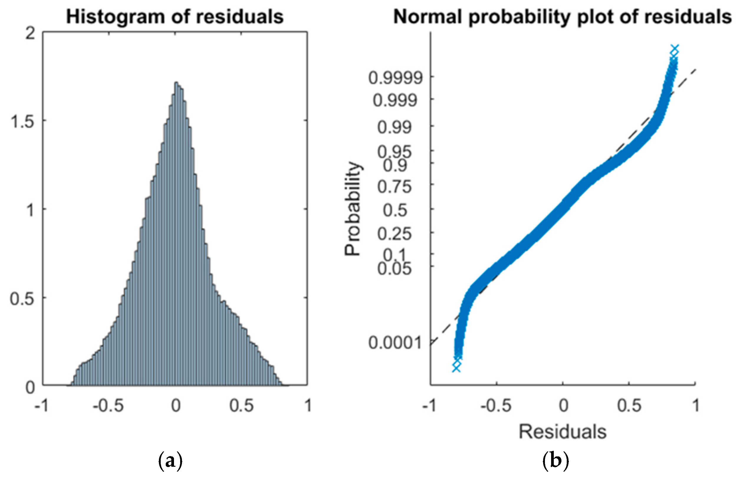
In this case, we eliminate 8618 outliers in order to improve the normality of the residuals, so the new distribution is as shown in
Figure 8. Although we have removed the residuals, it is still necessary to analyse the correlations between them so we can check the quality of the model.
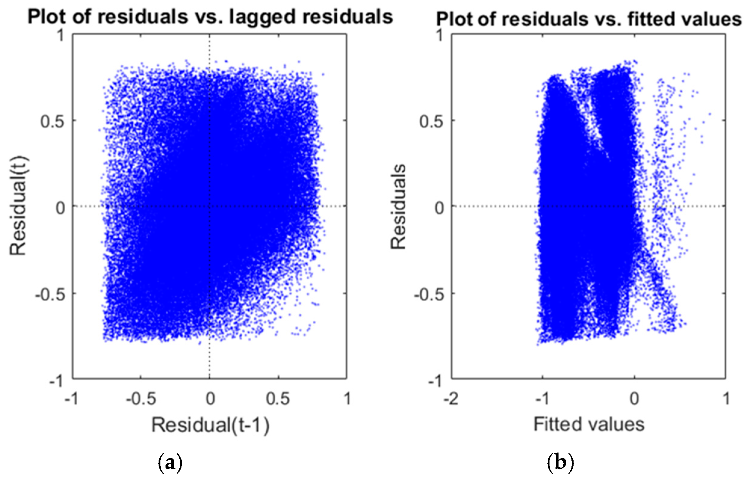
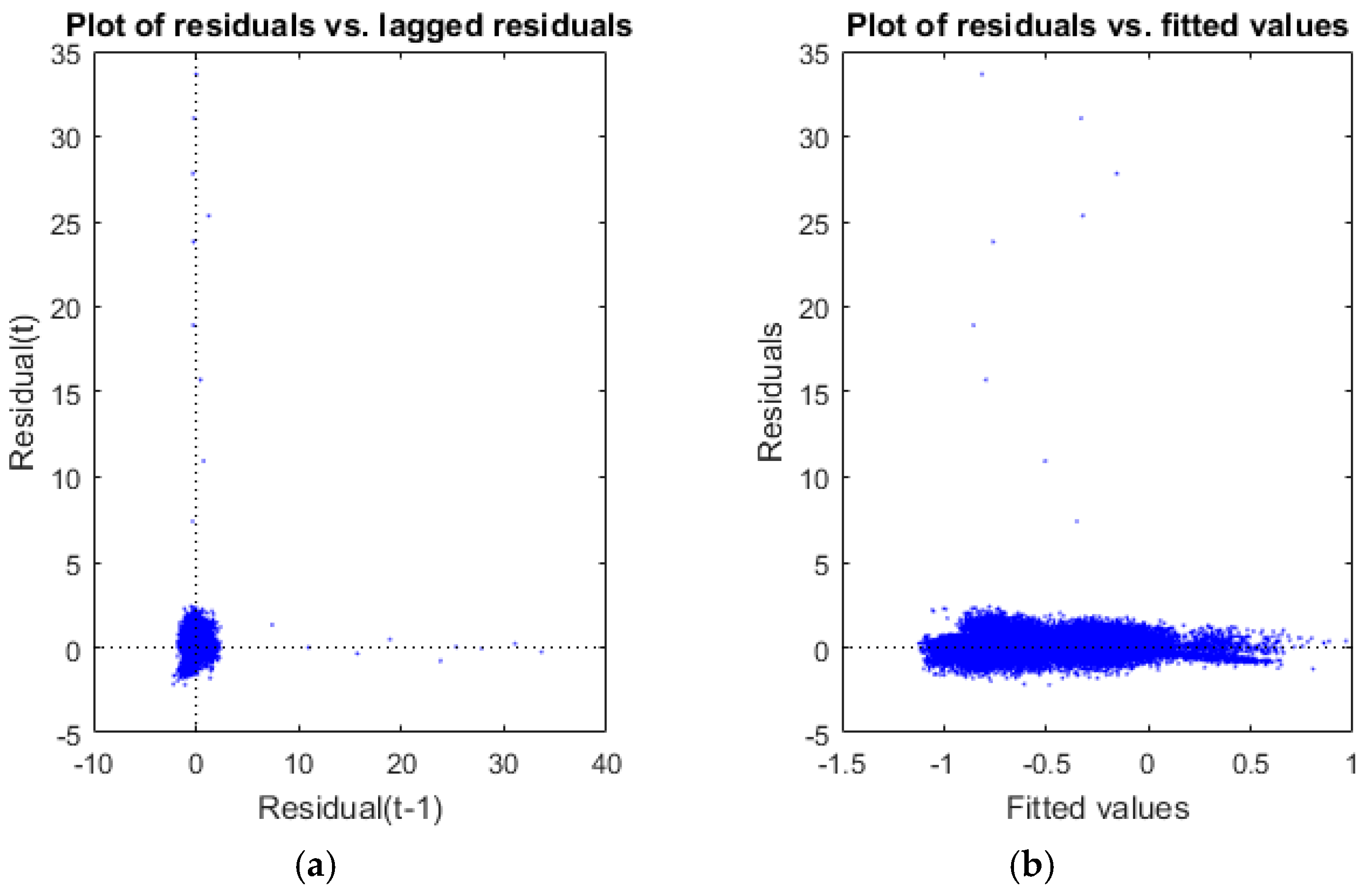
The scatter plot of residuals in
Figure 9 shows that there are neither positive nor negative relationships between residuals and lagged residuals. That means that there is no serial correlation among residuals. Furthermore, when a model is not well fitted, a clear tendency to have bigger residuals for bigger fitted values can be seen. In our case, the fitted values figure shows that the residuals are practically independent of the measured values.
Anyway, we perform a new phase of elimination of outliers, as
R-squared is still too low. Once the outliers have been removed, we still have
observations. In this new phase, the
, which is big enough for the model to be considered reliable.
Table 3 shows how the
p-values keep well below
.
In further attempts for a more complex model, we tried quadratic regression and log linear regression but did not produce coherent results as we obtained decelerations of the order of
, so we chose the model in
Table 3 to calculate the increase in the costs of fuel.
Analysis of the Selected Track
From the set of data of December 2015, we selected a long complex pattern based on inertia. The ideal pattern should have many phases of pure inertia, that is, without the use of brakes and braking periods. We selected one according to the number of inertia and braking phases and with a KPI close to the mean of all the patterns during the studied period. We chose one particular situation in which the driver performed a type #1 pattern with three phases of pure inertia and two braking periods. The total time of the pattern is 20 s, and during seven of those seconds the driver used the brakes. This would make
; this is a
of use of the brakes. The mean KPI for this type of pattern on this bus route and in the month of study is
, which makes the selected track an average one. The selection of this track fulfills the aim of this paper to estimate the potential savings of the use of inertia in the company as it compensates the peaks and troughs of performance by each individual driver.
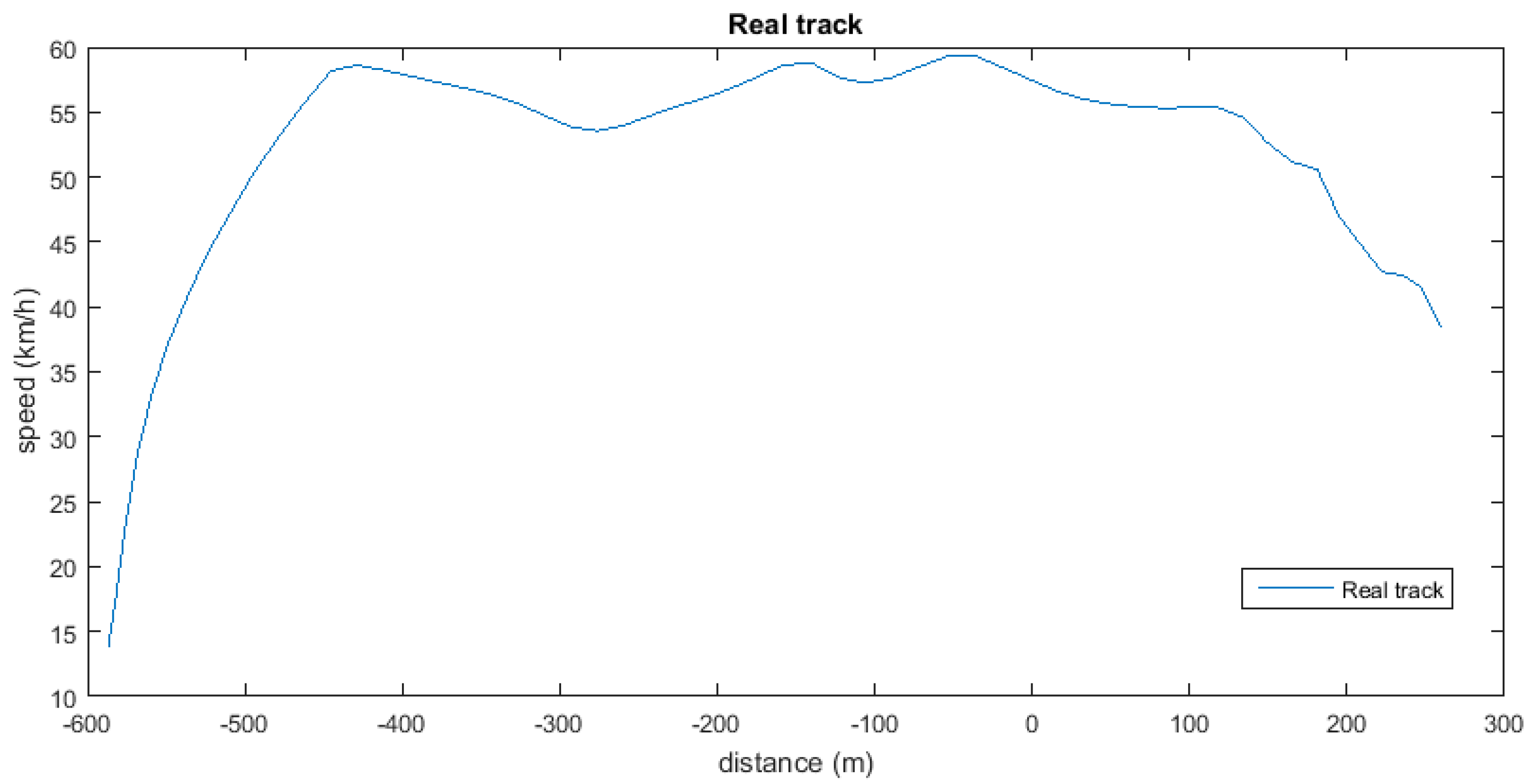
Figure 10 shows the representation of the pattern in terms of speed (
y-axis) and distance (
x-axis). Although the bus belongs to an urban transport company, speeds of over
implies that it is a non-urban road, which is quite common near the start and finish points of a bus route. In addition, the long distance indicates that the traffic is very light.
We have forced the point at the start of the pattern, so the “positive distance” is the non-consumption part of the track and the “negative distance” is where the vehicle consumes fuel. It could seem that inertia started before the “0” point, but we only have a reduction of speed due to the progressive release of the accelerator pedal by the driver. That makes a difference between deceleration, with consumption in this case, and inertia, always without consumption. Although in the part of the track prior to the start of the pattern there might be some null-consumption periods, as there are some decelerations, they are not relevant for the results as we will only add up the instant fuel consumption of all the samples included in the track.
To check the inefficiency of the real track, we apply the linear regression model, following these steps:
- (1)
Starting with the speed, engaged gear, engine regime, and position data at the last sample of the real track, we apply the linear regression model. The result is the simulated instant acceleration (negative) of the vehicle if the vehicle was using inertia.
- (2)
We calculate the speed of the vehicle in the instant of the previous sample.
- (3)
From the result of Step 2, and knowing which gear was engaged, we can obtain the engine regime and the distance travelled in the time elapsed between the last sample and the previous one.
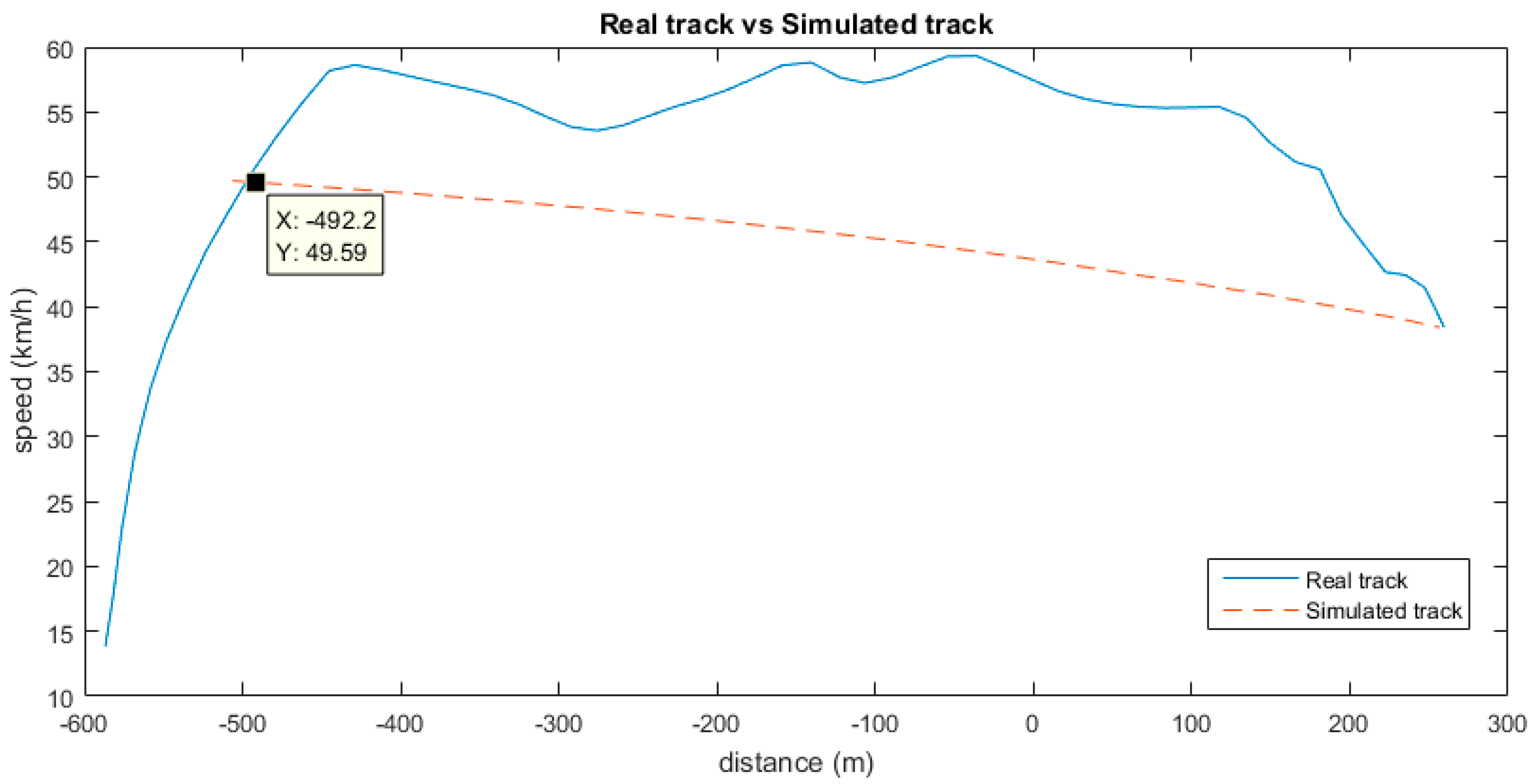
Now we have the data to apply the linear model, starting with Step 1 again. Therefore, we go back, calculating the ideal points of the simulated track. When we reach a point at which the ideal curve cuts the real one (ideal speed is higher than real speed), then we have the ideal starting point of inertia, as shown in
Figure 11. In that point, the position and speed are the same for both the real and ideal tracks. Therefore, we now know the domain of samples that we have to analyse. We know that the consumption in the simulated track is null, as the driver would be applying inertia. In order to quantify the inefficiency of the real track, we only need to calculate the total consumption of the bus in the real track. We have the instant consumption of each sample in
, and the elapsed time between every two samples in
, so for
samples we just need to apply:
With this approach, we could say that the driver would have saved of fuel if inertia had been used as proposed in our simulation. The case shown by the simulation is an extreme one, in which we do not consider the loss of time ( over the whole track), but it shows a good estimation of the potential savings if we managed to maximize inertia against continued accelerations and the use of brakes. The loss of time over a whole route of , which is this case, would be of 2 min and 44 s, extrapolating the data of the studied track.
According to the web site geoportalgasolineras.es of the Spanish Ministry of Energy, Tourism, and Digital Agenda, the fuel price in Gijon, the city where the case study takes place, varies from to (prices for the 5th of December 2016). If we use an average price of the saving in the track referred to in the case study would have been of . This result could be extrapolated to a longer period of time, for example, a month.
Considering that the KPI of the studied pattern is of use of the brakes, we could estimate the results for the whole route, which is long. Also, we consider the relation between the distance run during the pattern and the total length of the studied track. In this case, these values are and a total distance of the track of .
The total distance run in inertia in the studied route was of
, making an inertia distance ratio of
and a brakes use percentage of
. With this data, the total amount of money saved by a single vehicle on a complete route with an ideal usage of the brakes would be:
Considering that, according to our records, this vehicle completed 611 routes during the selected month, the company would have saved:
This would be the money saved by the vehicle that has been monitored for our study. On that route there is one bus every 15 min so, considering that the time spent to complete it is slightly over 45 min, there are four buses going from header 1 to header 2 with a break at the end of every run and another four buses going in the opposite direction. If we consider that those eight buses have the same characteristics, the total monthly saving for the company on the studied route would be of .
6. Discussion and Conclusions
With these results, we can see the importance of trying to anticipate different situations while driving. According to our records, only by applying inertia adequately can savings of of the total expenditure on fuel that the vehicle had during the month of study be achieved. Needless to say, this is an extreme top saving case, but it is a good theoretical estimation of the potential that efficient driving has in urban transport companies. It is important to point out that we used real consumption data directly obtained from the vehicle during working time in real conditions to make the calculations of the case study. It was not possible to verify the claims in a prepared test scenario as the vehicles are not available for off-duty activities, but the deceleration values obtained with the linear regression are very realistic, given the real data used to develop them.
These results are obviously limited to the conditions defined in the case study. The bus route, the weather conditions, which were very variable throughout the month, or the type of bus could also influence the final figures. Of course, the drivers using the monitored vehicle could have made a difference as well. Nevertheless, we consider that the results may be generalized since we did not apply the study to one particular driver and the objective of the paper is not the evaluation of drivers. In addition, we are aware of the seasonality of consumption. The selected month has the most similar consumption to the monthly average consumption, the consumption in July being the highest (69.70 l/100 km) and in January the lowest (61.26 l/100 km). Apart from that, the gathered data include peak hours on the one hand and weekends, with a very low density of passengers and traffic, on the other, so the whole spectrum of weight and traffic density range is considered.
The reliability of the mathematical model resides in the repeatability of results when conditions are the same. Thus, the use of several buses would have reduced this repeatability due to mechanical differences caused by each bus being a different model of different age or because each is involved in a different stage of maintenance. Our saving estimation for all the vehicles working in this route is still valid as they are all the same model, but if we apply the study on each bus, more precise results would be obtained.
We based the comparison of the study on the inertia patterns because they give a clear base (null consumption) to calculate the savings. In our previous work [
5], we defined other efficient driving patterns that also affect fuel consumption, but they are not so easily quantifiable as inertia. The reason is that we would have to compare their absence instead of their presence, as they represent inefficiency.
Regarding the complex inertia patterns, they showed very little variability in terms of consumption. They were originally designed to describe the behaviour of the driver, as it is not the same to exceed the use of the brakes while stopping as to do it when trying to adapt your speed to that of the traffic. However, all of the patterns and their KPIs show a similar structure when we are talking about expending fuel. This paper demonstrates that the exploitation of the vehicle’s inertia is enough to save fuel, but, depending on how well you use the previously gained energy, the savings could be much higher.
Any company applying an efficient driving methodology will achieve savings in fuel and money, as well as improving safety and comfort. Although our evaluation method is not directly based on fuel consumption, we conclude that it has proved to be very effective when it comes to reducing costs and improving the productivity of the company. In addition, this behavior based evaluation method could be a fair starting point for a reward system to incentivize the correct use of efficient driving techniques, as it would minimize dependence on the environmental parameters that affect fuel consumption such as seasonality or weight variations due to changes in passenger density when it comes to evaluating drivers’ performances. The findings in this paper would enable the companies and their drivers to envisage which techniques need revising and improving.
Future work aims to develop an automatic recommendation system that allows drivers to receive proper information about how to approach the ideal inertia performance indicated in this paper. We will also work with real data to see which combination of actions of the driver and efficient driving patterns would allow him/her to approach the ideal, simulated track without a loss of time.


 ,
, 


