1. Introduction
Since individual battery cells have limited voltage and capacity, power batteries require a variety of series or parallel combinations to achieve the voltage or capacity level for various applications [
1,
2]. However, due to manufacturing inconsistencies, and differences in the operating temperature and unique performance characteristics of each single cell, the cells connected in series may suffer from a serious imbalance between cell voltages or state of charge (SOCs) after many charging and discharging cycles [
3]. The imbalance of SOC can cause some of the cells to become overcharged or over discharged. This reduces the usable capacity of battery strings, shortens the lifetime, and even poses a safety hazard (e.g., an explosion or fire, etc.). Equalization for battery strings could be realized to prevent these phenomena and prolong battery string lifetimes.
Numerous equalization topologies and balancing methods have been proposed [
4,
5,
6,
7,
8,
9,
10,
11,
12,
13,
14,
15,
16,
17,
18,
19,
20,
21,
22,
23,
24,
25], and they are well summarized in [
5,
6,
7]. The equalization topologies are usually categorized as either passive or active circuits.
Passive equalization is the most straightforward and cheapest method. However, the excess energy is converted into heat rather than stored, which leads to energy waste and thermal management problems [
5,
7].
The active equalization circuits transfer energy to energy storage elements, such as capacitors, inductors and transformers. Thus, these active equalization circuits can generally be categorized as capacitor-based [
8,
9,
10,
11,
12,
13,
14], inductor-based [
15,
16,
17,
18,
19,
20,
21,
22,
23] or transformer-based [
24,
25,
26] circuits, each of which has its own advantages and disadvantages in terms of speed, accuracy, cost, size and efficiency.
With the advantages of small size, low cost, and easy control, switched-capacitor (SC) power conversion circuits are successfully used to equalize the cell voltages of series-connected battery strings [
8]. Resonant equalizers are also developed based on LC (inductor and capacitor) quasi-resonant circuits in [
12,
13,
14]. The equalizers based on LC quasi-resonant circuits can realize zero-current switching and reduce the switching loss of switches. However, the balancing speed of these circuits becomes lower when the cell voltage difference is small [
6,
8,
13]. Shang and Li have done some work to improve the balancing speed of LC quasi-resonant equalizers by using buck-boost converters to enlarge the voltage difference across the LC quasi-resonant converter, but it compromises on converters efficiency [
6,
13]. Transformer-based equalization circuits have a very high balancing speed and high level of integration, but they need a transformer with multiple outputs for all the cells. This transformer is expensive and difficult to design for a large number of cells [
3]. In addition, the transformer-based equalizers have poor expandability and large transformer magnetic flux leakage [
7,
15]. Thus, the transformer-based equalizers have difficulties to use in a large battery string. Inductor-based equalization circuits include buck-boost, Cûk, Sepic converters and so on. The equalization circuits proposed in [
15,
16,
17,
18,
19,
20,
21,
22] belong to this type. Inductor-based equalization circuits can realize bidirectional energy flow with higher balancing efficiency, but they often require a complex switch array and a precise control algorithm [
8,
24].
The topologies discussed above can solve the imbalance problem quickly if there are only a few cells in series. However, many of these equalizers suffer from long balancing times for a large number of battery cells. One reason why the balancing process is slow is that the equalizers are connected in series and the balancing speed is thus limited to the capacity of a single equalizer on the equalization path [
3,
15]. The balancing speed is not only related to the equalization topology, but also to the number of equalization path operating in parallel.
Parallel structures proposed in [
9,
10,
15,
16,
24,
25] have a faster equalization speed, but the transformer-based parallel structures [
25,
26] have design difficulties for a large number of cells. To expand the equalization path, Han has proposed a parallel architecture equalizer (PAE) based on buck-boost converters for battery strings in [
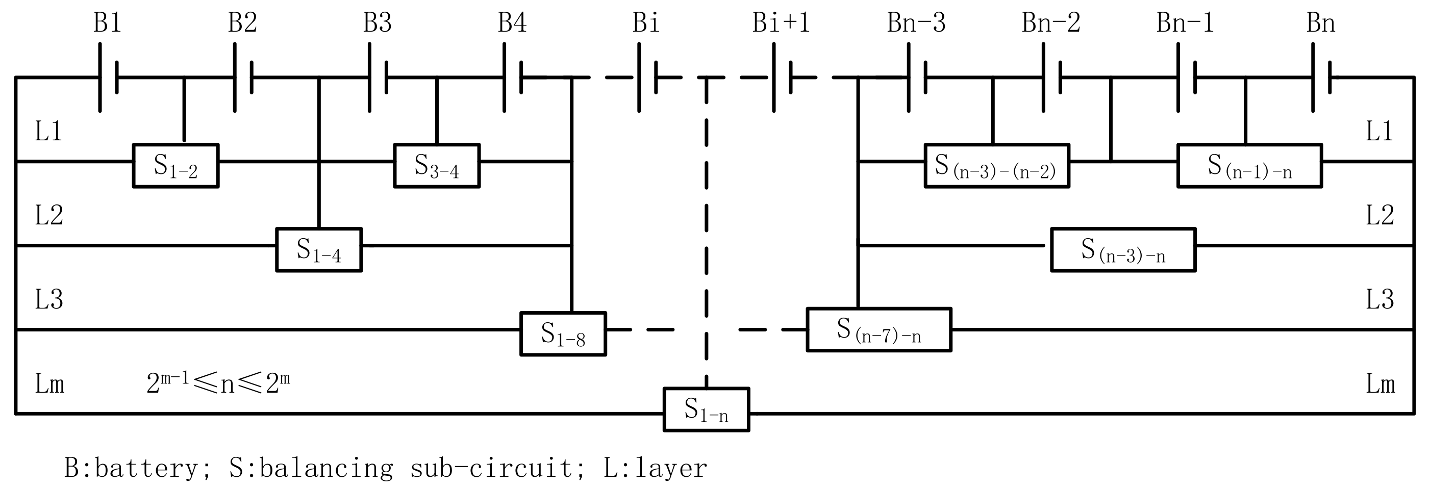
15], as shown in
Figure 1. In the PAE, all the balancing sub-circuits are placed in parallel layers. All the layers can equalize their corresponding cell groups simultaneously. Han has done a systematic comparison between parallel architecture equalizer (PAE) based on buck-boost converters, traditional inductor-based adjacent equalizer (IBAE) [
18], parallel architecture equalizer based on a multi-wind transformer (PAEBMWT) [
25] and double-tiered switched-capacitor equalizer (DTSCE) [
10]. The comparison results show that the PAE has a good performance in balancing speed, balancing efficiency, and control complexity. The balancing time of PAE is the shortest, and it can be reduced by 50%, compared with IBAE. In addition to PAE, some parallel architecture equalizers realized by switched-capacitor converters [
8,
9] and switched-inductors [
16,
20] will be introduced in detail in
Section 4.
In consideration of the advantages and disadvantages of the equalization methods discussed above, a novel inductor-based layered bidirectional equalizer (IBLBE) with the advantages of series-parallel connected balancing path and high level balancing speed is proposed. The main idea of the IBLBE is modularizing the battery string with layered balancing circuits based on buck-boost converters to realize fast active equalization in different layers synchronously, especially for large battery strings. The IBLBE has a higher level balancing speed than other equalizers based on switched-capacitor or switched-inductor converters.
In this paper, the IBLBE is proposed and analyzed. Its circuit structure and equalization principle are introduced in
Section 2. The models and calculation of the key parameters are derived in
Section 3. In
Section 4, the simulation results and comparison with several existing equalizer are presented. The experimental result is shown in
Section 5, followed by the conclusion in
Section 6.
2. Proposed Equalizer Scheme
2.1. Structure of the Proposed Equalizer
Figure 2 shows the system configuration of the proposed equalizer.
Figure 2a is the structure of the equalizer;
Figure 2b is the schematic diagram of the bottom balancing circuit;
Figure 2c is the schematic diagram of the balancing sub-circuit.
The battery string connected in series is subdivided into N modules, and each module contains n individual cells. The N battery modules are divided into two parts with cutoff point K. If N is an even number, N = 2 × K; if N is an odd number, N = 2 × K − 1. Every battery module Mi is equipped with a balancing sub-circuit Ei, which controls the charge transfer between Mi and other modules. Each battery module is divided into two parts with cutoff point k. If n is an even number, n = 2 × k; if n is an odd number, n = 2 × k − 1. Every individual cell is equipped with a balancing sub-circuit Si, which controls the charge transfer between Bi and other individual cells in this module.
The balancing sub-circuits Ei and Si are implemented by buck-boost converters, which allow bidirectional energy flows. The balancing sub-circuits Ei compose the upper balancing circuits, which are used to achieve the equalization between battery modules. The balancing sub-circuits Si compose the bottom balancing circuits which are used for equalization between cells in each module. The upper layer circuits and the bottom layer circuit are connected in parallel and can be operated simultaneously, which extends the balancing path and can achieve fast equalization for a large series connected battery string.
The proposed equalizer IBLBE can achieve the dynamic adjustment of equalization path and equalization threshold, described as follows:
• Dynamic adjustment of the equalization path
The balancing sub-circuit Ei provides equalization path for module Mi, and the balancing sub-circuit Si provides equalization path for individual cell Bi. Each balancing sub-circuit can be operated independently according to the specific algorithm, which is determined according to different requirements. For instance, the equalizer operates Ei(s) in upper layer and Sj(s) in bottom layer concurrently to realize fast active equalization for a large battery string. Furthermore, the Sr and St (suppose Br and Bt are in the same module, VBr > > , r, j, t = 1, 2, …, n) can be operated synchronously to balance the most overcharged cell Br and most undercharged cell Bt at the same time.
• Dynamic adjustment of equalization threshold
The equalization circuits have two equalization thresholds; one for the battery modules and the other for the individual cells in the same module. If the two thresholds are not met, the balancing circuits stop working.
The working condition for the upper layer circuitsis , s are the modules terminal voltages. In each battery module, the working condition for the bottom layer circuitsis , s are the terminal voltages of cells in the same module.
The equalization thresholds could be adjusted according to the system requirements and the accuracy of sampling circuits [
1].
2.2. Equalization Principle
2.2.1. The Equalization Principle of the Bottom Layer Circuits
We use four battery cells connected in series as an example to elaborate the equalization principle of the bottom layer circuits. Firstly, we identify the highest and lowest cell voltage; secondly, we control the corresponding sub-circuit to transfer energy from the cell with the highest voltage to the others in the same module and from the other cells to the one with the lowest voltage synchronously. Suppose that the cell
B1 is with the highest voltage and cell
B4 has the lowest voltage in the module
M1. The equalization principle with two consecutive stages is shown in
Figure 3:
Stage 1: charge L1 and L4.
As shown in
Figure 3a, the switches
S1a and
S4a are first turned ON. The individual cell
B1 charges the inductor
L1; the
B1,
B2 and
B3 connected in series charge the inductor
L4. The inductor
L1 and
L4 store energy with the current
and
gradually increasing. Some of the electrical energy is transferred into magnetic energy stored in the inductors.
Stage 2: discharge L1 and L4.
As shown in
Figure 3b, the switches
S1a and
S4a are turned OFF. The inductor
L1 charges cell
B2,
B3 and
B4 through the flywheel diode of
S1b; the inductor
L4 charges cell
B4 through the flywheel diode of
S4b. The most overcharged cell
B1 and most undercharged cell
B4 are balanced at the same time. Furthermore, the balancing current does not only flow through
B1 and
B4 but also flows through
B2 and
B3. This accelerates the balancing process compared to other equalizers.
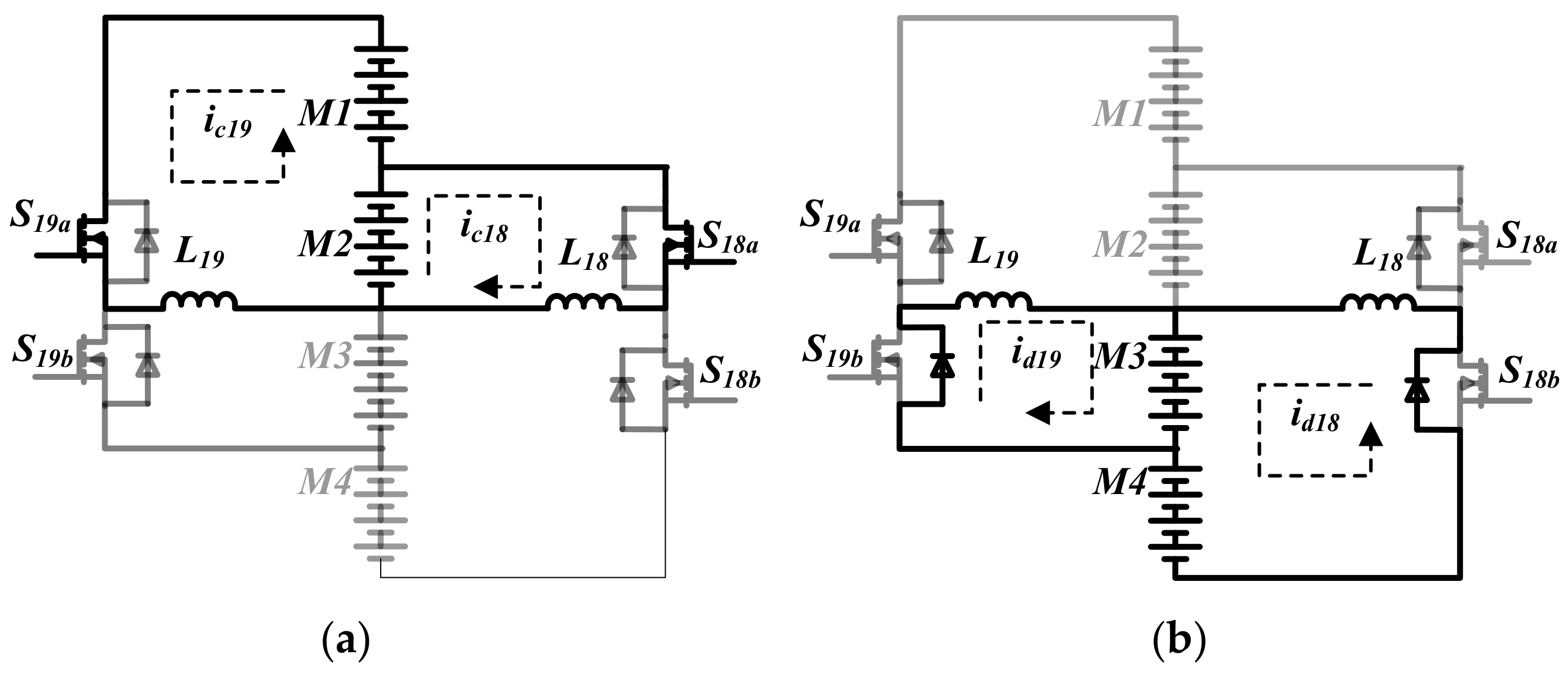
2.2.2. Equalization Principle of the Upper Layer Balancing Circuits
Use four battery modules connected in series as an example to elaborate the equalization principle of the upper layer circuits. The module M2 is assumed to be overcharged and the module M3 is under charged.
As shown in
Figure 4a, switches
S18a and
S19a are first turned ON. The
M2 charges the inductor
L18;
M1 and
M2 charge the inductor
L18. Then, as is shown in
Figure 4b, the switches
S18a and
S19a are turned OFF. The inductor
L18 charges the module
M3 and
M4 through the flywheel diode of
S18b and the inductor
L19 charges module
M3 through the flywheel diode of
S19b.
3. Modeling, Analysis and Calculation of the Key Parameters
In this section several key parameters are analyzed including the balancing current, the inductors current, duty cycle of switch waveform, the switching frequency and the inductances.
3.1. Modeling of Inductor Current and Duty Cycle of Driving Waveform
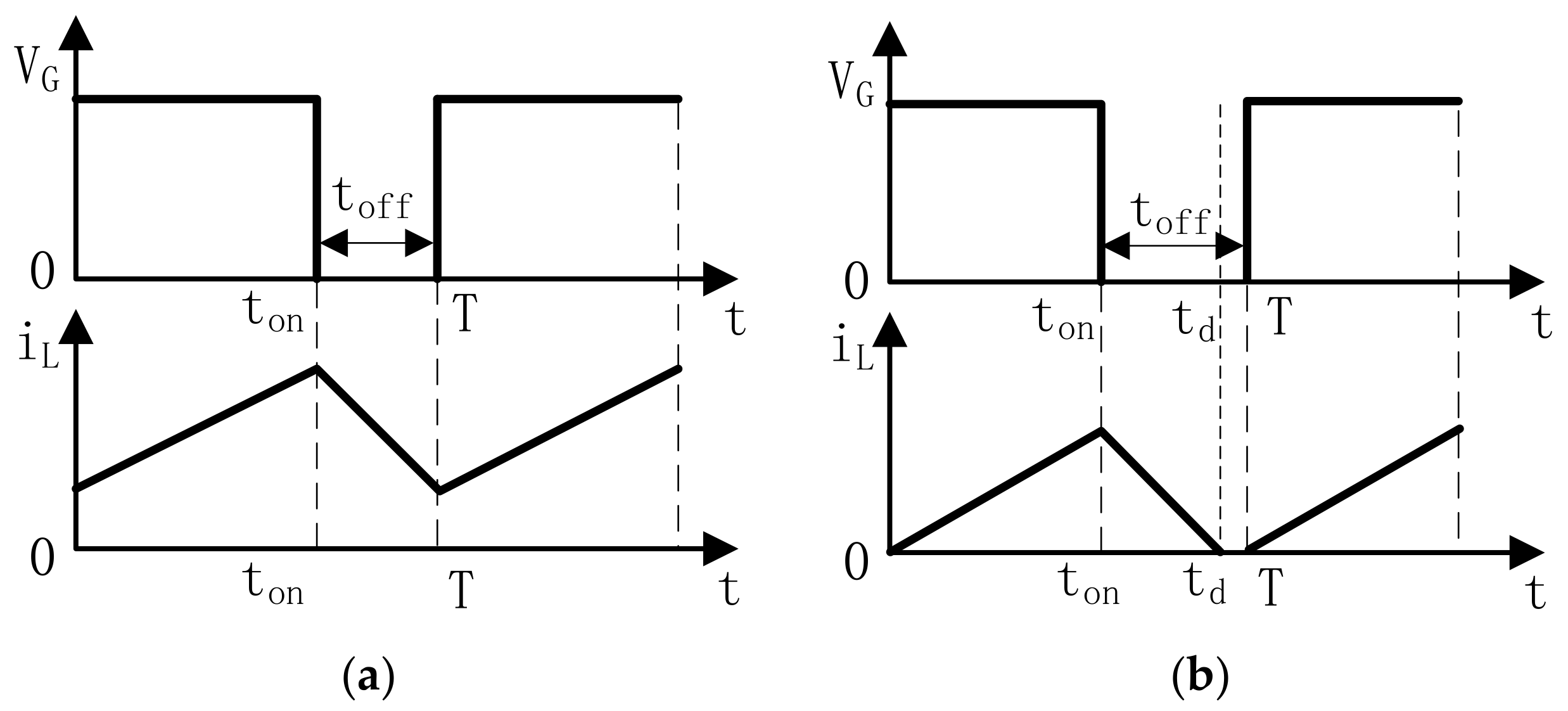
DC-DC (direct current) converters have two working modes: continue current mode (CCM) and discontinuous current mode (DCM), shown in
Figure 5. The CCM has a large inductor current with feedback control [
15]. Considering the magnetic saturation and the complexity of control, DC-DC converters work in the DCM in this paper. In DCM, the inductors can release all absorbed energy in the off-time of the switches and the converters is without current sensors and feedback control [
20].
During the energy transfer process of the inductor
Li, denote the voltage across
Li by
Vc when the switch is turned ON, namely the total cells voltage charging
Li; denote the voltage across
Li by
Vd when the switch is turned OFF, namely the total cells voltage discharging by
Li:
In which, is the inductor current, VD is the forward voltage across the body diode of MOSFET, Ron is the loop total resistance when the switch is turned ON, Roff is the loop total resistance when the switch is turned OFF, td is the moment that inductor current falls to zero.
This is a first order full response circuit, and the inductor current response is:
In (5),
ip is the peak value of inductor current
. The resistances
Ron,
Roff and
VD are ignored since their values are very small. Then the inductor current increases linearly when the switches are turned ON; the inductor current decreases linearly, when the switches are turned OFF:
In (7),
D represents duty cycle, and
T represents switching period. To make the DC-DC converters working in the DCM, the inductor current need drop to 0 in the off-time of switch. The conditions that the duty cycle need satisfy are derived as follows:
when
; since
, when
:
3.2. Inductance, Switching Frequency and Equalization Time
The cell-balancing time is a key indicator for equalizer need to be considered. This problem can not only be solved by improving the equalizer topologies but also by increasing the balancing current. This is because the amount of charge transferred from one cell to others in unit time is proportional to the average value of current through the cell [
8]:
In which, ΔQ is the energy transferred from one cell to the others in one second, iBiavr is the average current through Bi, T is the switching period and f is the switching frequency. In equalization process, the current in balancing circuit is derived as follows:
The peak value of inductor current:
The average value of inductor current:
In the balancing sub-circuit
Si, the average value of the cell
Bi:
The average value of inductors current is proportional to the product of D2 and Vc or D(1 − D) and Vc; is inversely proportional to the product of L and f. The values of D and Vc cannot adjust at will. The balancing time is inversely proportional to the average value of balancing current, shown in Equation (9), therefore, the balancing time of IBLBE is proportional to the product of L and f. In that case, the selection of L and f can achieve different levels of the balancing current and balancing time. Increase the switching frequency f can reduce the volume of inductors and improve equalizer integration. The impact of equalizer topology and the initial distribution sequence of the cells charge will be further discussed in next section.
4. Simulation
The simulation model of the proposed equalizer is built in PSIM9.0. In order to reduce the balancing time, 10F capacitors are employed to substitute battery cells [
8,
14] with initial voltage shown in
Table 1. The switching frequency is set as 10 kHz. Cell balancing based on voltage inconsistency is more easily implemented and more common [
15,
20,
22]. In this paper, the cells terminal voltages are employed as the index of inconsistency.
It is assumed that the capacitors, inductors and switches are all lumped element. Moreover, the influence of parasitic inductance and parasitic capacitance and the deviation generated by AD (anolog to digital) transfer are ignored.
SOC (%): SOC values corresponding to each cell voltage are for a 2.6 Ah Sanyo ternary lithium battery. VBmax = 3.961 V, VBmin = 3.852 V, maximum voltage gap is 109 mV, maximum SOC gap is 15%. VMmax = 15.676 V, VMmin = 15.587V, maximum voltage gap is 89 mV.
4.1. Equalization Simulation for IBLBE and PAE
4.1.1. Equalization Simulation for IBLBE and PAE with 4 Cells
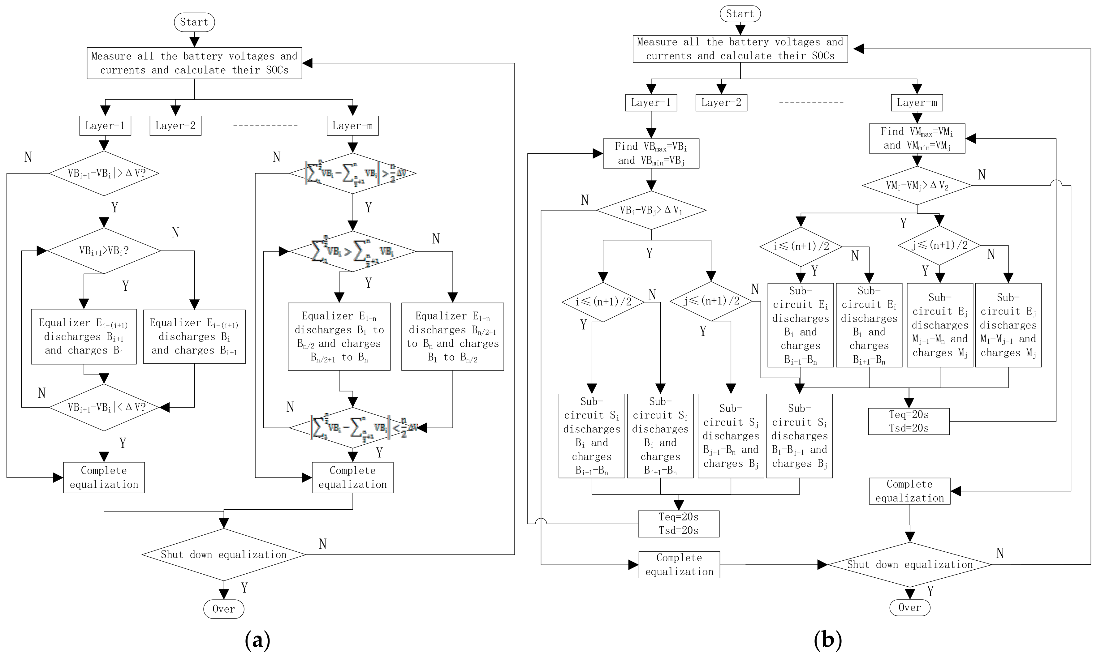
The circuit diagrams and the equalization flow charts of the two equalizers are shown in
Figure 6 and
Figure 7. The balancing time of the two topologies both depend strongly on the initial distribution sequence of the cells’ charge. In fact, some charge transferred from one cell to another occurs directly; in other cases, the charge transferred from one cell to another only occurs after multiple transfers between groups of cells. Therefore, the balancing time depends on the initial distribution sequence of the cell charges.
A statistic work has been done to obtain the average balancing time in different initial distribution sequence of the cell charges for PAE and IBLBE. Take the four cells battery string as an example. The number of different distribution sequence is
, and only 12 are independent samples. The initial voltages of the four cells are A = 3.961 V, B = 3.935 V, C = 3.909 V, D = 3.871 V, the values of SOC are 65%, 61%, 57%, 53% for a 2.6 Ah Sanyo ternary lithium battery. Set the equalization threshold as 3 mv for the two equalizers.
Table 2 shows the 12 independent samples and their balancing time in PAE and IBLBE.
Table 3 shows the comparison between PAE and IBLBE in 4 cells battery string. The proposed equalizer IBLBE uses two more MOSFETs and one more inductor than PAE. In the 12 independent samples, there are nine samples in which the balancing time of IBLBE is shorter than PAE. The IBLBE reduces balancing time by 29% in average. The balancing time variance of IBLBE is much smaller than that of PAE, which means the IBLBE has a relatively stable balancing time than PAE in different initial distribution sequence of the cell charges. In PAE, the balancing time is usually longer when the voltage difference in the first layer equalizer becomes larger, such as ADBC, ADCB, BCAD, DABC.
Furthermore, the IBLBE can use more different algorithms than PAE since all the balancing sub-circuits in IBLBE are independent.
4.1.2. Equalization Simulation for IBLBE and PAE with 16 Cells
The initial voltages of cells and modules are shown in
Table 1. We built layered balancing circuits for IBLBE and PAE to compare the balancing speed between IBLEB and PAE with a 16 cell battery string. The 16 cell battery string is divided into four battery modules, and each module has four cells connected in series.
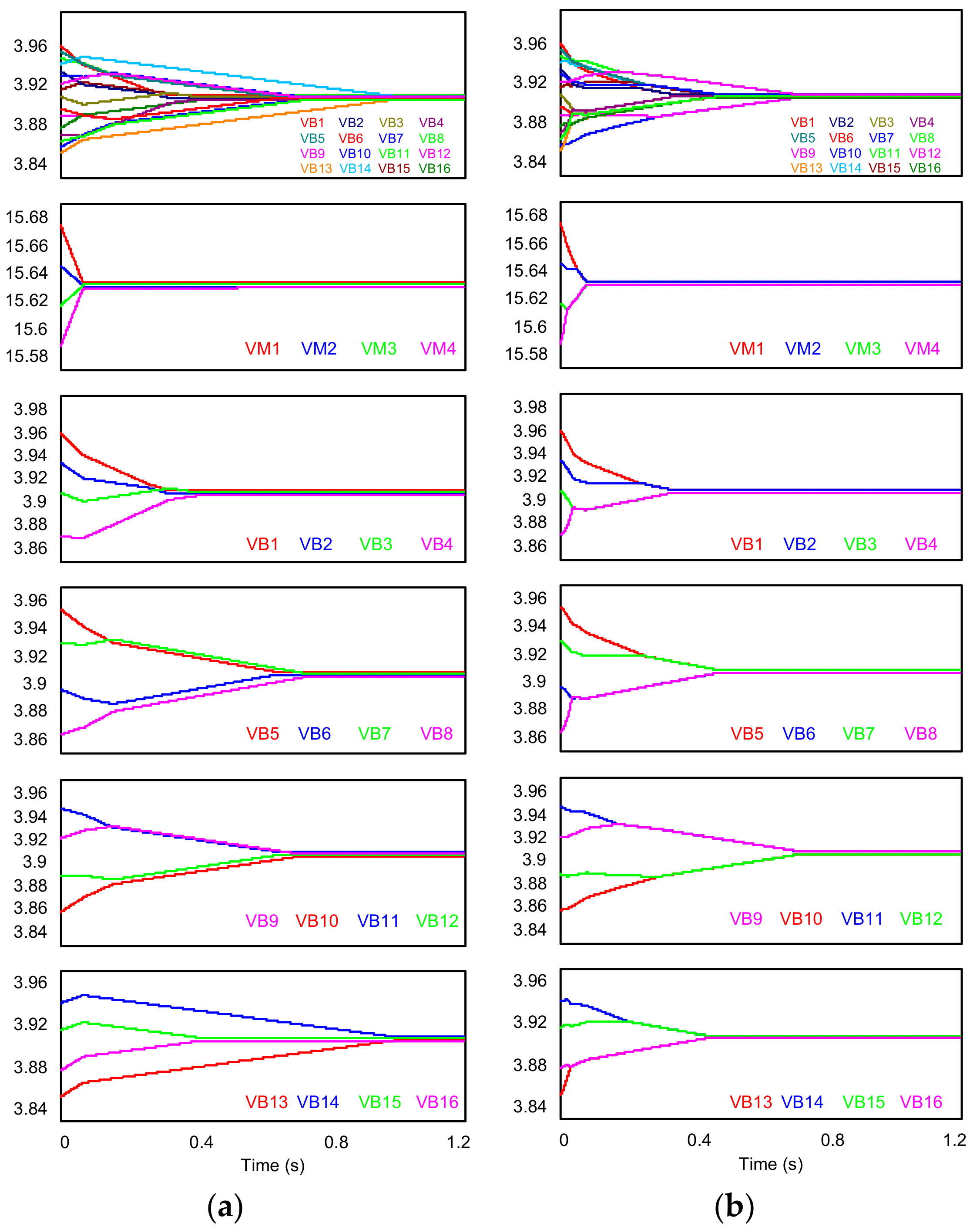
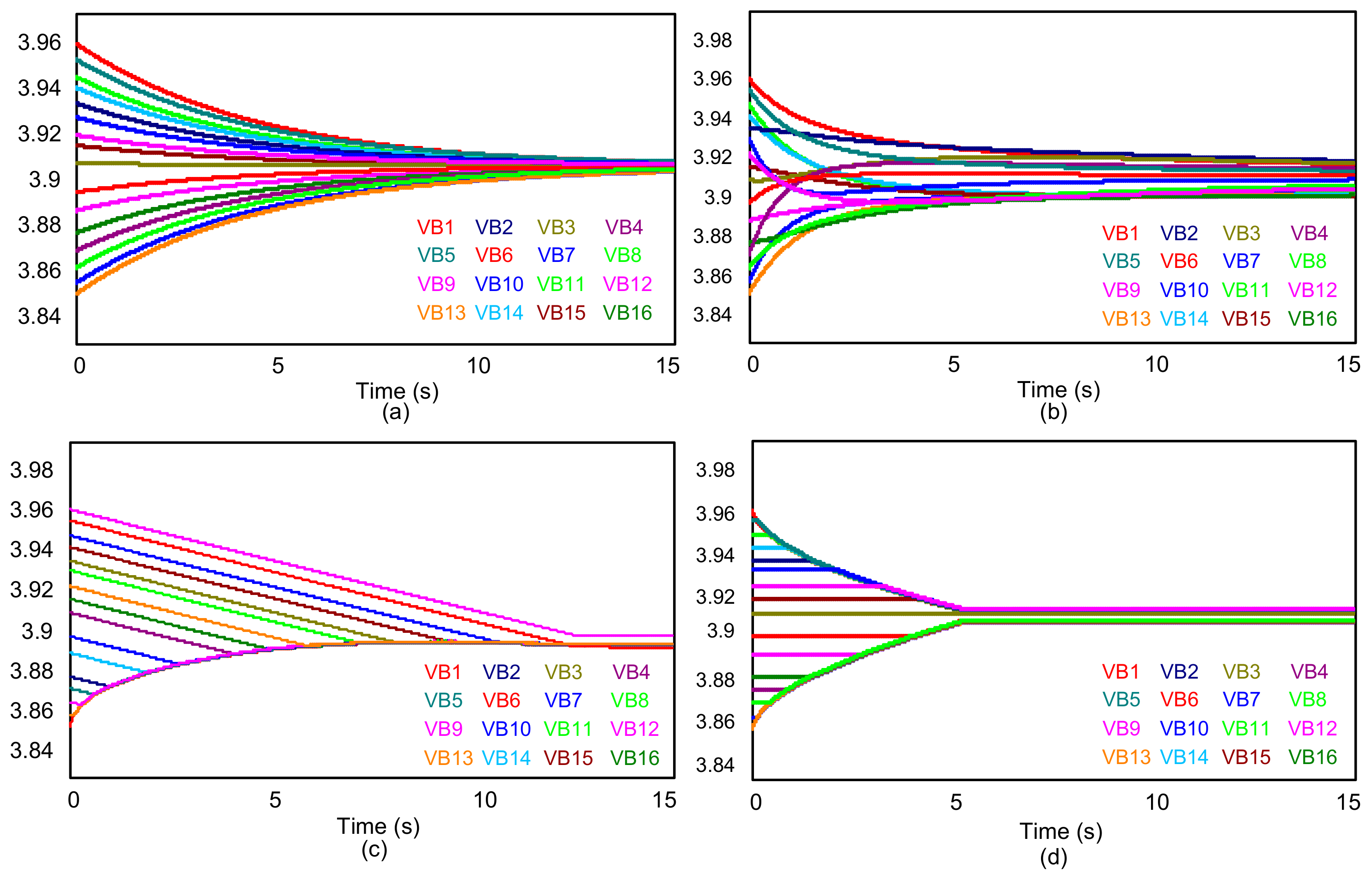
Figure 8 presents the cell voltages trajectories in PAE and IBLBE. As is shown in
Figure 8, the IBLBE stops equalization at about 0.7125 s, and the PAE stops at 0.9969 s. The equalization between four battery modules is much faster than the equalization in the bottom layer (or the first layer).
In
Figure 8a, the slowest battery module is M4, and its balancing time is 0.9969 s which puts off the whole PAE equalization process. In
Figure 8b, the slowest battery module is
M3, and its balancing time is 0.7125 s, which equals the whole balancing time of IBLBE. In module
M1, the balancing speed of IBLBE is faster than PAE. In module
M2 and
M3, the balancing time is the same in PAE. The IBLBE is a little bit slower than PAE in
M3, but it is faster than PAE in
M2.
Thus, the balancing time for the whole battery string depends on the slowest battery module. The balancing time for each battery module depends on the initial distribution sequence of cell charges. The IBLBE can achieve faster active equalization than PAE, because the balancing time fluctuation of IBLBE is much smaller than that of PAE in different distribution sequence of cells charge and the expected balancing time of IBLBE is shorter than PAE. For example, the module M4 stops equalization at 0.9969 s in PAE, but it only needs 0.4332 s in IBLBE.
To quantitatively evaluate the expected balancing time for the two topologies with 16 cells battery string, the statistical model is simplified in this paper. Suppose that the initial charges of cells are the same in different modules, but the distribution sequence is different. Thus, balancing operation only occurs between cells in each module and not occurs between battery modules. The whole balancing time depends on the slowest module. As shown in
Table 2, the PAE has three independent samples for four cells; IBLBE has about four “independent” samples for four cells (the samples with similar speeds are sorted into the same independent sample). After probabilistic and statistical computing, the expected balancing time of IBLBE is 0.6531 s, the expected balancing time of PAE is 0.9311 s. IBLBE reduces the expected balancing time by about 30%.
4.2. Equalization Simulation for Other Topologies with 16 Cells
Han has done some comparisons between PAE [
15], IBAE [
18], PAEBMWT [
25] and DTSCE [
10]. The comparison results showed that the PAE balancing time of PAE is the shortest, and it can be reduced by 50%, compared with IBAE. Furthermore, the PAE has good performance in balancing efficiency, and control complexity. In this part, some further comparison between switched-capacitor-based equalizer (SCBE) [
8], chain structure switched-capacitor equalizer (CSSCE) [
9], single switched-inductor equalizer (SSIE) [
21] and buck-boost-and-LC-resonant based equalizer (BBLCRE) [
13] has been presented. The equalization process of the four equalizers is shown in
Figure 9.
Table 4 presents the comparison between different equalizers. The SCBE proposed by Ye and Cheng, has a simply topology and its balancing speed is independent of both of the number of battery cells and initial distribution sequence of cell voltages. However its balancing speed is much slower than IBLBE. The balancing time of SCBE is 21 times longer than that of IBLB. The CSSCE can’t realize accurate equalization between 16 cells or a large number of cells during an acceptable time. The BBLCRE has excellent performance in balancing efficiency, but the balancing speed is slow. The balancing speed of BBLCRE is proportional to the voltages difference across LC resonant converter, but the balancing efficiency is inversely proportional to it. Thus, balancing efficiency and speed, the BBLCRE can’t have both. In addition, it needs more relays than other topologies. When the V out of the buck-boost converter is set to 4.5 V, and the ideal efficiency of LC resonant converter is about 86.7%. In this case, the balancing time of BBLCRE is 12 times longer than that of IBLBE. The SSIE uses only one inductor. However, this equalizer has a complex switch matrix which needs to operate four switches in a loop in each switching period and it takes a long time to serve all cells in a long battery string with only one balancing bypass. Furthermore, the balancing time of SSIE is about eight times longer than that of IBLBE.
5. Experimental Results
In order to further verify the equalization principles and show the balancing performance of the proposed equalizer, a balancing system is implemented and tested with sixteen 2.6 Ah Sanyo ternary lithium batteries.
Table 5 summarizes the parameters of IBLBE. The inductances and the resistances in
Table 5 are measured by a TH2810D LCR Meter (Tonghui, Changzhou, China). The initial cell voltages and SOCs are shown in
Table 1.
In every equalization cycle, the equalization time teq = 10 s, and the standing time tsd = 10 s. The standing time in every equalization cycle is aimed at eliminating the polarization voltage of cells. Therefore, it is more accurately to test the real open-circuit voltages (OCVs) of cells, and issue the balancing instructions.
Figure 10a shows the experimental waveforms of inductors current
and
and the duty cycle of PWM is 65%;
Figure 10b shows the experimental waveforms of inductors current
and
and the duty cycle of PWM is 24%. The inductors current is discontinuous and varies in saw-tooth waveform. The peak value of
comes to 2.2 A; the peak value of
is about 2.1 A; the peak value of
is 2.5 A; the peak value of
is about 2.2 A. These agree with the theoretical analysis in
Section 3.
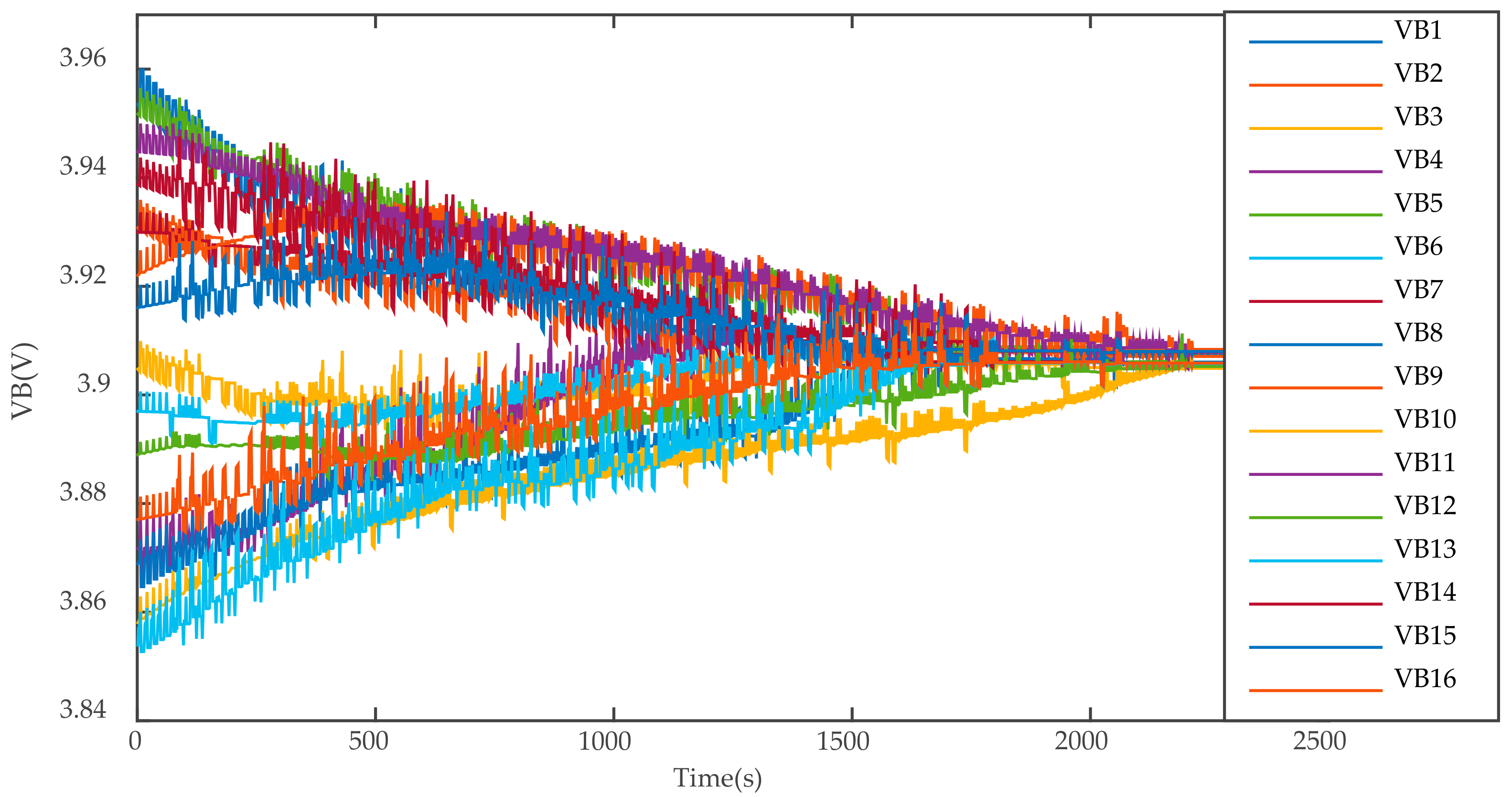
Figure 11 shows the 16 cells’ voltage trajectories in the equalization process.
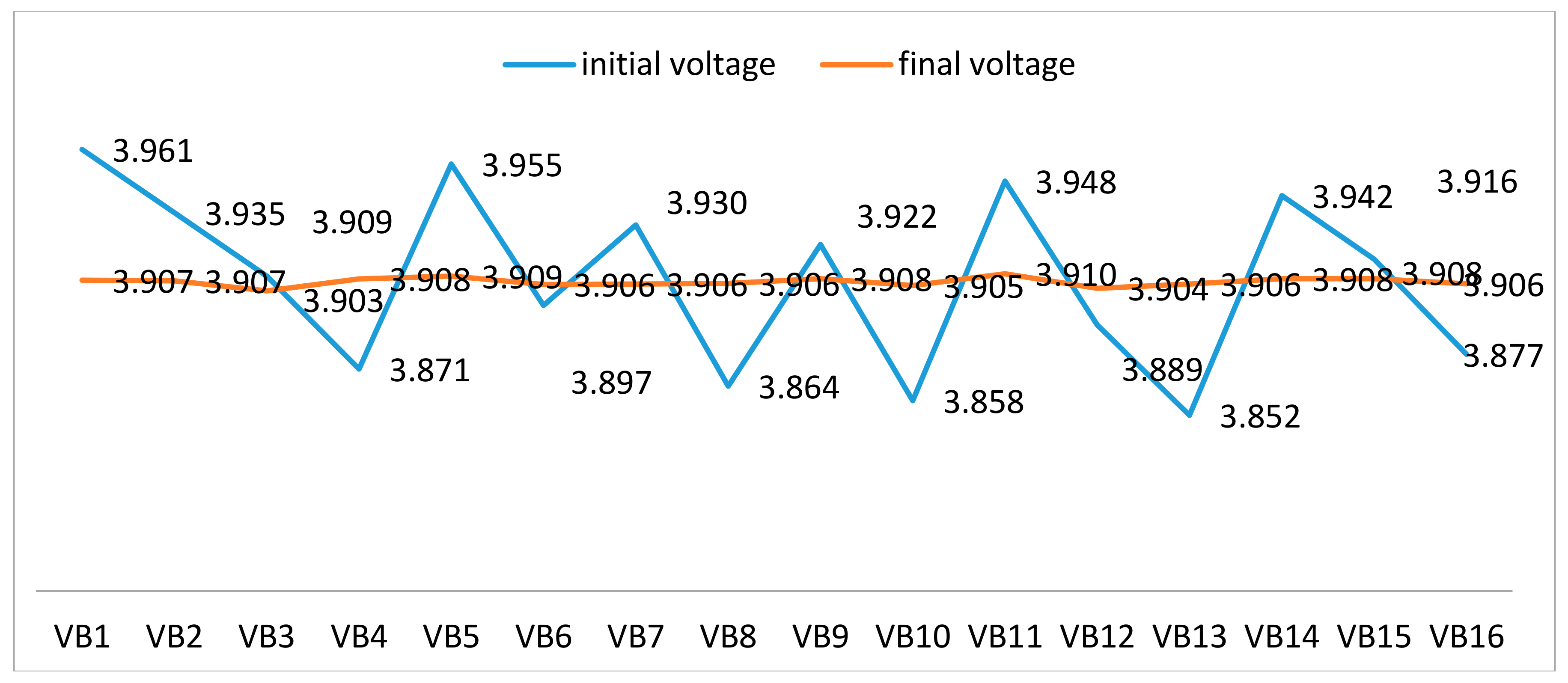
Figure 12 presents the 16 cells’ voltage before and after equalization. The initial voltage gap shown in
Table 1 is 103 mV, and it decreases to 8 mV at about 37 min.
The initial SOC gap is 15%, and the final SOC gap decreases to 1.2%. The accuracy of the equalization is excellent. The balancing time in
Figure 11 agrees with the simulation result in
Figure 8b after an equivalent calculation method.


