
Sensible Heat Transfer during Droplet Cooling: Experimental and Numerical Analysis
by
 , , and
Emanuele Teodori
1 ,
,
Pedro Pontes
1,
Ana Moita
1,
Anastasios Georgoulas
2,*,
Marco Marengo
2 and
Antonio Moreira
1
1
IN+ Center for Innovation, Technology and Policy Research, Instituto Superior Técnico, Universidade de Lisboa, Av. Rovisco Pais, Lisbon 1049-001, Portugal
2
Advanced Engineering Centre, School of Computing, Engineering and Mathematics, Cockcroft Building, Lewes Road, University of Brighton, Brighton BN2 4GJ, UK
*
Author to whom correspondence should be addressed.
Energies 2017, 10(6), 790; https://doi.org/10.3390/en10060790
Submission received: 25 February 2017
/
Revised: 2 June 2017
/
Accepted: 5 June 2017
/
Published: 9 June 2017
(This article belongs to the Special Issue Advanced Thermal Simulation of Energy Systems)
Abstract
:This study presents the numerical reproduction of the entire surface temperature field resulting from a water droplet spreading on a heated surface, which is compared with experimental data. High-speed infrared thermography of the back side of the surface and high-speed images of the side view of the impinging droplet were used to infer on the solid surface temperature field and on droplet dynamics. Numerical reproduction of the phenomena was performed using OpenFOAM CFD toolbox. An enhanced volume of fluid (VOF) model was further modified for this purpose. The proposed modifications include the coupling of temperature fields between the fluid and the solid regions, to account for transient heat conduction within the solid. The results evidence an extremely good agreement between the temporal evolution of the measured and simulated spreading factors of the considered droplet impacts. The numerical and experimental dimensionless surface temperature profiles within the solid surface and along the droplet radius, were also in good agreement. Most of the differences were within the experimental measurements uncertainty. The numerical results allowed relating the solid surface temperature profiles with the fluid flow. During spreading, liquid recirculation within the rim, leads to the appearance of different regions of heat transfer that can be correlated with the vorticity field within the droplet.
1. Introduction
1.1. Objectives
The present work aims to experimentally measure the temperature field of a heated surface during the impact of a cold droplet with high temporal and spatial resolution. The results obtained are then used to benchmark a coupled solver based on the volume of fluid (VOF) method that accounts for conjugate heat transfer (CHT) between the solid and fluid regions. It is expected that further insight on the characteristic mechanisms of sensible heat transfer, will be given.
1.2. Motives
Droplet cooling in the non-boiling regime is an efficient cooling method. Most of the studies reported in the literature usually quantify the heat transferred using measurements at a single point i.e., at the centre of the impact. Such measurements, are not very useful for the validation of numerical studies, since they are limited to a finite number of measuring probes. On the contrary, the present work compares numerical predictions with experimental results where the entire temperature field resulting from droplet cooling is numerically resolved and experimentally measured.
1.3. Research Importance
Directly comparing experimental and numerical temperature fields can lead to a deeper understanding of the principal heat transfer processes. The high spatial-temporal resolution achieved in the experimental measurements is extremely useful for a deeper evaluation of the present as well as other numerical solvers. Once the solver is benchmarked it allows a detailed description of the flow field of the impinging droplet. The relation of the flow field with the temperature field can allow a better description of the underlying heat transfer mechanisms.
1.4. Research Questions
The present investigation aims to answer the following research questions:
- Is it possible to reproduce high spatial-temporal resolution experiments numerically? If yes, which are the limitations?
- Can the numerical results describe properly the sensible heat transfer in droplet cooling?
- How is the flow field within the droplet connected with the heat removed?
- Gap in knowledge 1: Validation of a numerical solver has never been conducted comparing high resolution, transient, experimental and numerical results for the entire temperature field that is developed in the solid region during the droplet impact.
- Gap in knowledge 2: The relation between the flow field within the droplet and the heat removed during droplet spreading has not been accurately described yet.
1.5. Literature Review
Droplet/spray cooling of a heated surface usually occurs by the impact of single or multiple cold droplets on a heated surface. Many authors try to take advantage from boiling and evaporation of the droplets/sprays impinging onto the surface to be cooled [1]. However efficient cooling can be obtained also relying only on the sensible heat removed from the droplet without the occurrence of phase change. Even in this case, heat transfer coefficients as high as 24,000 W/m2·K [2] and up to 660,000 W/m2·K [3] have been reported in literature, thus confirming that even without boiling, the sensible heat transfer during droplet impact is still suitable for cooling applications.
Studying a relatively simpler system based on a single droplet can be useful to properly describe the physics of complex cooling systems based on multiple droplets impact. In this context, the fluid dynamics of a droplet impacting onto a rigid surface has been widely investigated. Extremely useful reviews and descriptive papers are available on the topic [4,5,6,7]. It is well known that when a single droplet impacts a solid surface, different outcomes can occur. Namely, the droplet can spread, disintegrate (splash) or bounce from the surface after impact. These outcomes depend on the impact conditions (impact velocity and size of the droplets), on the liquid and surface properties and conditions related to temperature and wettability. High speed imaging is usually used to characterize the collision dynamics of a liquid droplet on a solid surface. The pioneer work from [8] showed the capabilities of this technique and since then several authors e.g., [9,10,11] used high speed photography to analyse different parameters affecting the phenomena of droplet impact.
Although droplet collision on a surface has been extensively studied, an accurate description of the combined heat transfer and fluid dynamics mechanisms is not a trivial task. In the non-boiling cooling regime, a strong variation of temperature occurs in the surface due to the convective heat removal at the first instants after impact. After this stage, heat is removed mainly by evaporation of the droplet. Many authors have investigated the heat transfer during droplet impact onto heated surfaces e.g., [12,13]. However, the usual quantification of the heat transfer in the majority of these works, is based on surface temperature measurements at the centre of the impact to the surface only, using thermocouples.
1.6. State of the Art
High spatial and temporal resolution measurements of the temperature field in the heated surface can be a valid alternative to single point measurement, to properly describe the underlined heat transfer mechanisms during droplet impact. Examples of experimental techniques that allow this kind of measurements are micro heaters [14,15] thermocromic liquid crystals [16] and laser-based thermo-reflectance [17,18].
Another technique that is being increasingly used within the last years is infrared thermography. This technique was used to measure the evolution of the temperature field of an impacting droplet during evaporation, for example in [19]. These authors provided temperature measurements of the surface/droplet interface. They could highlight differences in the temperature between the centre and the periphery of the droplet. In [20], the authors monitored the liquid-solid interface temperature after droplet impact through an infrared transparent material. They could confirm typical trends of droplet cooling and properly measure the distribution of temperature at the droplet-solid interface. These studies were focused on the evaporative heat removal of the droplet. Droplet evaporation occurs in a relatively long time scale (seconds), so the authors could use an IR camera with about 25–60 Hz acquisition frequency. Higher acquisition frequency is required to focus on the sensible heat removed during droplet impact in the spreading stage (milliseconds), which can be achieved with high-speed infrared thermography as proposed in [21]. The authors focused on the resulting temperature field of the surface during droplet impact, spreading and recoil. Using high-speed thermography and high-speed visualization, they could infer on the effect of surface wettability and on the improved cooling performance of nanofluids, when compared to base fluids without the nanoparticles. In [21], the authors could measure the temperature field of the bottom side of the surface and quantify the sensible heat removed during droplet impact. Other examples of the use of IR thermography are the studies of [22] and [23]. In [22] the authors measured the surface temperature during droplet impact in the Leideinfrost regime, while in [23] measurements of the temperature field of the liquid/air interface in the droplet film during impact onto a heated surface, are reported.
The numerical reproduction of the heat transfer between a surface and impinging droplets can also give further insight in the mechanisms occurring during droplet impact. In this context [24], proposed the “Marker and Cell” (MAC) finite difference method to solve the Navier-Stokes equations. Despite being a pioneer work, the MAC code originally implemented, needed some modifications to account for heat transfer which were further introduced in [25] and [26]. Other methods have been used to solve numerically the problem of drop impact onto heated surfaces such as the Lagrangian approach [27]; the Immersed Boundary Method (IBM) [28,29] and the Level Set (LS) methodology ([30,31]). In [30], the authors highlight different regions of heat flux along the radial direction of the impacting surface, which can be related with the flow in the lamella (the radial liquid film formed as the droplet spreads) and in the rim, surrounding the lamella. Particularly, a dip in the heat flux was noticed close to the droplet rim when the film becomes thinner and thus unable to remove as much heat as the other regions of the spreading droplet. In fact, despite being recognized by many authors that the lamella has an irregular shape, e.g., [32], such shape, including the flow within the rim are sparsely considered, e.g., in [33]. The authors in [30], also emphasised that the heat removed during the spreading of the droplet is not negligible, despite the short characteristic time intervals addressed (maximum of tens of milliseconds).
The LS method employed by [30] uses a continuous distance function to indicate the distance from any point in space to the free-surface. Similarly, the volume of fluid (VOF) method tracks the motion of the free surface by introducing a VOF function. Differently from the LS method the VOF function distinguishes the liquid region from the gas region using the discrete values 1 and 0 respectively. The interface is in this case identified by values between 1 and 0. Therefore, the volume fraction indicates the fraction of a computational cell that is occupied by liquid.
Using VOF methodology Pasandideh-Fard et al. [34], could simulate the impact of a water droplet onto a hot stainless steel surface. They did not account for phase change in the droplet, since the temperature of the substrate was kept lower or just slightly above the boiling temperature. They presented numerical results for pressure, velocity and temperature distributions within the droplet and temperature distribution within the heated solid. The authors in [34], highlighted an irregular distribution of the temperature and of the heat flux along the radial direction of the droplet. They benchmarked their solver by comparing their results with experimental data obtained using a single thermocouple placed at the centre of impact of a stainless steel heated surface.
More recently in [35], a VOF-based approach was also used. The authors solved the conjugate problem of fluid flow and heat transfer during the impact of water droplets onto a heated surface. They performed simulations at moderate surface temperature to prevent nucleate boiling. Evaporation of the droplet was considered using a Fick’s law-based, local vaporisation rate formula. Liquid properties were a function of local temperature. The authors reported a region of high heat flux close to the contact line. They related the presence of this region with higher evaporation rates occurring in the contact line.
Despite the completeness of the different models proposed so far in literature, their validation was based on comparison only with experimental measurement of temperatures at the centre of droplet impact. Instead, the present investigation, according to the authors’ best knowledge, addresses for the first time a more detailed benchmark process, in which the entire calculated temperature field of the surface in contact with the spreading droplet is compared with the temperature fields obtained experimentally, for different time instants during droplet impact and spreading. The experimental data were gathered combining high speed IR thermography of the temperature field of the heated surface, with high speed visualization of the droplet impinging process.
It is expected that through this process, further insight will be provided regarding the underpinned mechanisms of heat transfer, especially in the spreading stage of droplet impact. Moreover, potential limitations in the comparison between numerical and experimental results can be highlighted. Main emphasis is put on the sensible heat removed by the droplet and in how the flow field of the droplet can be related with heat and mass transfer phenomena. In fact, the post-processing and analysis of the numerical results reveals for the first time, a relationship between the local heat transfer coefficient and the vorticity field within the spreading droplet.
2. Materials and Methods
2.1. IR Thermography—High Speed Visualization Set-Up
The experimental set-up consists of an infrared IR high-speed camera (MWIR-InSb, ONCA 4696 series from Xenics, Leuven, Belgium) placed below the heated target, a high-speed camera (Phantom v4.2, Vision Research Inc., Wayne, NJ, USA) placed at the side of the heated target, a power source for electrically heating the target, a syringe pump and a needle from which the droplet falls onto the heated target. The falling height, i.e., the vertical distance from the tip of the needle to the surface was varied to set the desired impact velocity. For instance, for an impact velocity of 2 m/s (Weber number We = 151) the needle was placed at 20 cm from the surface. The real impact velocity was then checked, following the procedure described in Section 2.2. A LED light source is placed in front of the high-speed camera at a distance of 15 cm from the point of impact onto the heated target. At this distance, the LED does not heat the falling droplet.
The heated target is a foil of stainless steel electrically heated. The foil is characterized by a thickness of 20 µm, a width of 20 mm and a length of 70 mm. Wettability is assessed measuring the static and the quasi-static advancing and receding contact angles, using an optical tensiometer (THETA from Attension, Biolin Scientific Holding AB, Stockholm, Sweden). The measured static contact angle was θ = 81.7° ± 1°. The quasi-static angles were used to evaluate the hysteresis of the foil, which was always larger than 20° ± 1° for the hydrophilic foils tested here. It is worth mentioning that despite the argument that advancing contact angles are more representative for the spreading motion of the droplet e.g., [36,37], as explained by [38], quasi-static angles are still static angles and accurate measures of dynamic angles are very difficult to obtain [37]. In the present work, measurements of the advancing and receding contact angles were characterized by low repeatability (standard deviation ±6°, maximum deviation from the mean value 12°). The applicability of the theoretical functions to derive advancing angles can also fail in the spreading analysis [39]. Therefore, for the numerical simulations of the present work, the accurate static contact angle was used to finally assess the surface wettability.
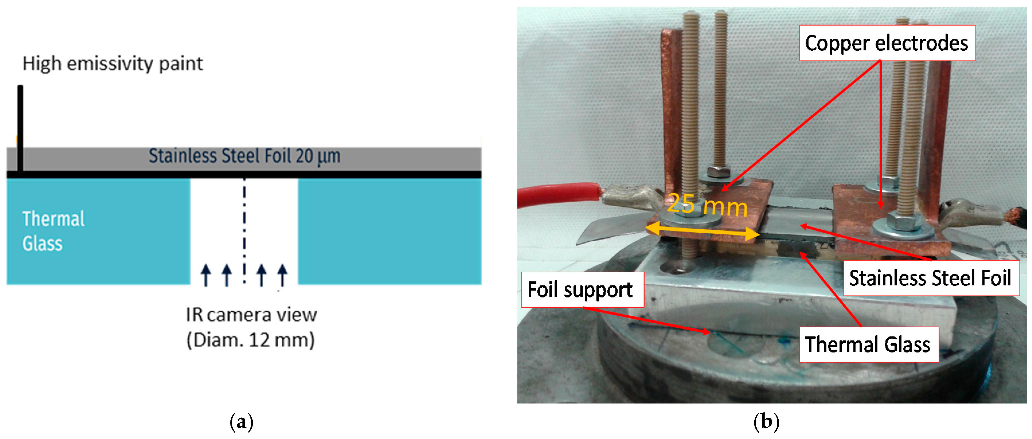
Once characterized, the foil is placed in a heating assembly that consists of copper electrodes clamped on top of the stainless-steel foil which is then glued on top of an insulating thermal glass. The whole assembly is then placed on a stainless-steel support (foil support) for an easier positioning. The bottom side of the stainless-steel foil used for IR thermography is black matt painted to increase the emissivity (ε = 0.95). A schematic view and a picture of the set up are reported in Figure 1, while an illustrative view of the heating assembly and foil positioning are reported in Figure 2.
2.2. Experimental Methods
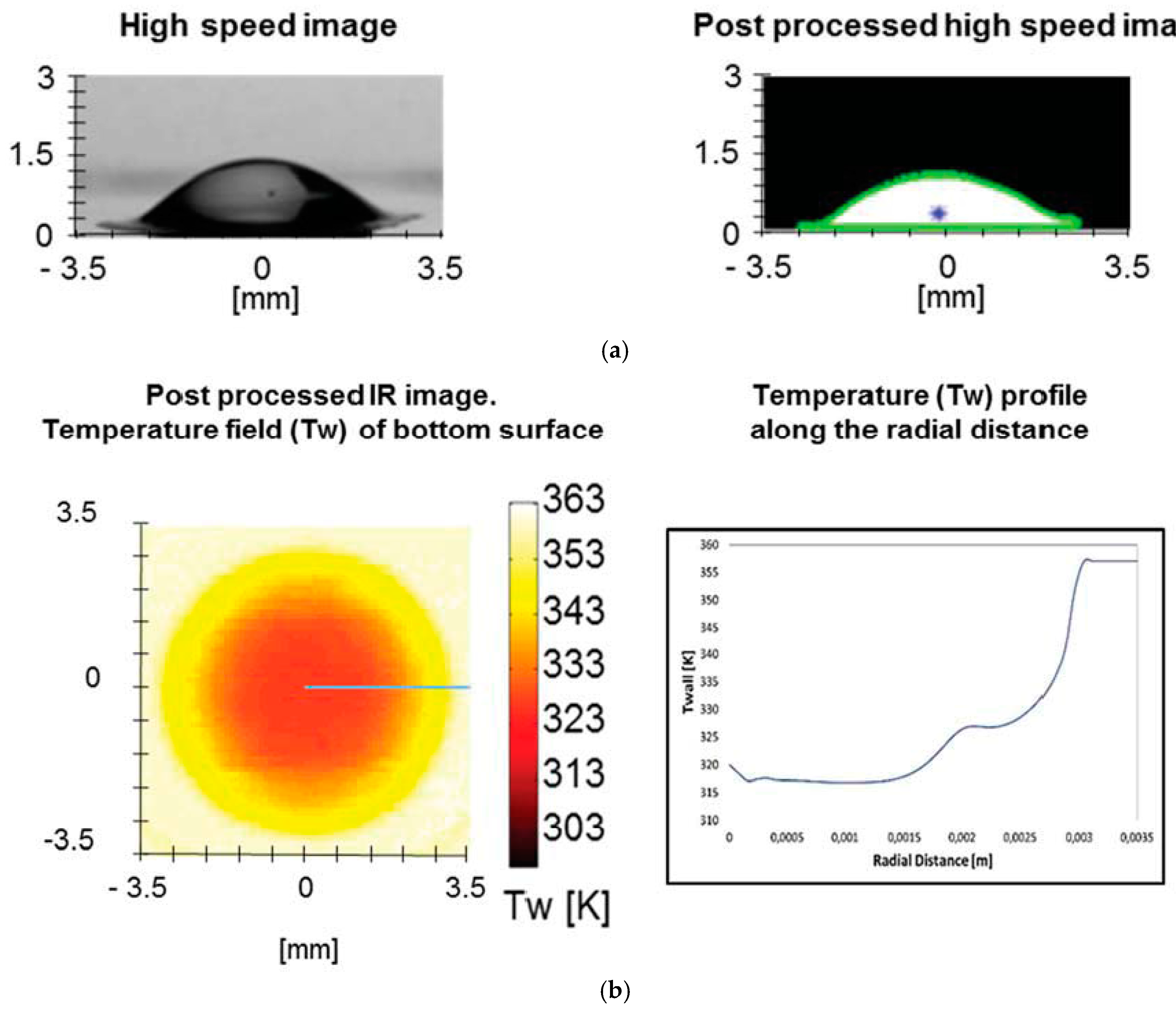
Water drop impact tests were performed for Weber numbers, We = 24–151 (see Equation (1)), initial surface temperatures Tw(in) =333.15–373.15 K and ambient temperature Tamb = 293 ± 2 K. The droplet diameter before the impact was = 2.6 ± 0.1 mm. The temperature of the droplet before impact was assumed to be equal to the ambient temperature. The test consisted in electrically heating the stainless-steel foil up to the desired temperature and then let the droplet impact on it, by action of gravity. During droplet impact, simultaneous but not synchronized high-speed and high-speed thermography images were recorded. The acquisition frequency and resolution were 2000 fps and 512 × 512 px2 for the high-speed images and 1000 fps and 150 × 150 px2 for the IR images. For each experimental condition considered here, five tests were performed to assure reproducibility of the experiments. Care was taken to assure that the initial surface temperature and wetting conditions were reproducible before each new droplet impact. The radial temperature profiles were obtained after post processing the IR images using a custom made, in-house developed MatLab code which allowed conversion of the raw IR images to temperature data. The high speed images were used to evaluate the spreading diameter i.e., the contact diameter and impact velocity using a code previously developed MatLab [40]. An example of the IR post processed images, temperature profiles as well as the raw and post-processed high speed images, is shown in Figure 3.
From the post-processed high-speed images, the spreading factor is evaluated as the ratio between the contact diameter at the liquid-solid interface, and the diameter of the droplet previous to the impact , ( (-)).
The impact velocity was evaluated by image post processing, as the vertical displacement of the droplet before impact divided by the time elapsed (i.e., three successive frames of the high-speed video). From the impact velocity and the diameter measured previous to impact, the Weber number We was obtained as:
where is the liquid density, is the impact velocity and is the liquid surface tension.
Radial profiles of temperature were obtained from the post processed infrared images. However, since the experimental conditions considered different initial foil temperatures a dimensionless temperature was used to remove the influence of the initial temperature of the surface and of the ambient temperature in the results. This dimensionless temperature is defined as:
where is the temperature of the bottom of the foil (wall) at time after impact and distance from the center of the droplet. is the initial temperature of the surface and is the ambient temperature. Temperature profiles are obtained plotting as a function of the dimensionless radial distance .
The imposed volumetric heat rate was evaluated as follows:
where and are correspondingly the applied voltage and resulting current passing through the stainless-steel foil and , , and are the thickness, length and width of the foil, respectively.
2.3. Measurement Uncertainties
2.4. Numerical Methodology
A VOF-based approach was used for interface capturing. In more detail, a previously enhanced VOF model implemented in OpenFOAM CFD Toolbox [41] is further coupled with an energy equation that accounts for two-phase heat transfer in the a fluid domain and with transient heat conduction in a solid domain.
In the VOF method a volume fraction field α identifies the volume of liquid within a cell. The volume of the gaseous phase is calculated as (1 − α). The value of α is 1 inside the pure liquid cells, 0 in the pure gas cells and between 0 and 1 in the cells containing the interface area. This procedure allows using a single set of continuity and momentum equations for the entire flow domain:
Continuity equation:
Momentum equation:
The volume fraction α is advected by the flow field using the following equation:
Interface sharpening is very important in simulating two-phase flows of two immiscible fluids. In OpenFOAM the sharpening of the interface is achieved artificially by introducing the extra compression term in Equation (6) (). Ur is the artificial compression velocity which is calculated from the following relationship:
where nf is the cell surface normal vector, φ is the mass flux, Sf is the surface area of the cell, and Cγ is a coefficient the value of which can be set between 1 and 4. Ur is the relative velocity between the two fluid phases due to the density and viscosity change across the interface. In Equation (6) the divergence of the compression velocity Ur, ensures the conservation of the volume fraction α, while the term α (1 − α) limits this artificial compression approach only near the interface, where 0 < α < 1 [42]. The level of compression depends on the value of Cγ [42,43]. For the simulations of the present investigation, initial, trial simulations indicated that a value of Cγ = 1 should be used, in order to maintain a quite sharp interface without at the same time having unphysical results.
It should be mentioned that the VOF method in OpenFOAM does not solve Equation (6) implicitly, but instead by applying a multidimensional universal limiter with explicit solution algorithm (MULES). Together with the interface compression algorithm, this method ensures a sharp interface and bounds the volume fraction values between 0 and 1 [44].
Energy equation:
where stands for the fluid velocity, the pressure and the temperature. Gravitational forces are represented as while represents the volumetric surface tension forces. , , and are the thermal conductivity, the density, the dynamic viscosity and the heat capacity of the bulk fluid, respectively. These are calculated as the weighted averages over the two phases according to the value of , using the following relationship:
where and are the liquid and gas properties, respectively.
The fluid energy equation (Equation (8)) does not account for evaporation or diffusion of the liquid phase in the gas phase. This approximation is considered valid in the relatively small time scales that are investigated here. In fact in [30,34] the authors conclude that heat transferred by evaporation of the droplet during spreading is negligible.
The VOF-based solver that is used in the present investigation has been modified accordingly in [41] in order to account for an adequate level of spurious currents suppression. The proposed modification involves the calculation of the interface curvature κ using smoothed volume fraction values that are obtained from the initially calculated volume fraction field , smoothing it over a finite region near the interface:
All other equations are using the initially calculated (non-smoothed) volume fraction values of α. The proposed smoothing is achieved by the application of a Laplacian filter which can be described by the following equation:
In Equation (11), the subscripts P and f denote the cell and face index respectively and is the linearly interpolated value of α at the face centre.
The Continuum Surface Force (CFS) method proposed in [45] is then used to model the surface tension as a volumetric force:
where is the surface tension.
Heat is transported only by conduction in the solid. Therefore, the energy equation in the solid domain can be expressed as:
where the subscript “s” indicates that the properties are of the solid only. The volumetric heat source is represented as and is considered as a property of the solid domain. It is constant and homogenously distributed in every single cell of the solid domain, with a value that coincides with the experimentally measured one.
2.5. Numerical Set Up
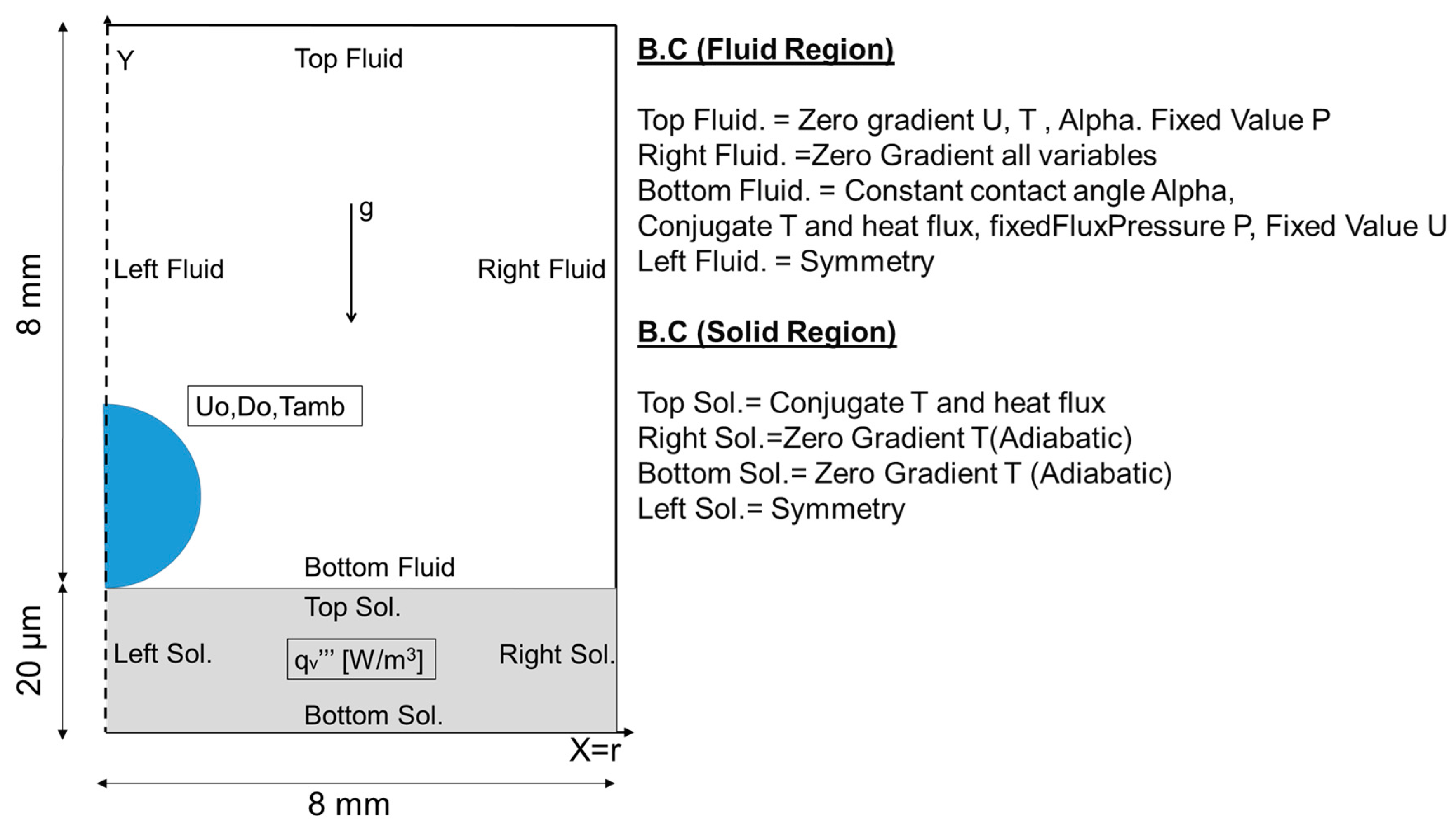
The set of equations previously listed, is solved in an axisymmetric domain, represented by a 5° wedge. An 8 × 8 mm2 fluid domain in the X-Y plane was chosen to avoid the influence of the boundaries in the fluid flow. The solid domain dimensions were 8 × 0.020 mm2 (20 µm thickness of the heated foil). The mesh consisted of 640,000 hexahedral cells in the fluid domain and 4000 in the solid domain. In the fluid domain, the mesh progressively coarsens away from the initial droplet position by a grading factor of 5 in both X and Y directions (last to first cell dimension in each direction is equal to 5). This leads to a minimum cell size of 4 μm and a maximum cell size of 20 μm. These cell dimensions were selected, for the solution to be mesh independent. Before every simulation an arbitrary thermal boundary layer was patched in the domain to facilitate the initial convergence of the coupling between the solid and liquid temperatures. A droplet with the same diameter and velocity as the experimental conditions was patched as well, at the time instant just before it touches the heated surface. The solid was considered as a volumetric heat source. Constant contact angle was assumed between the fluid and the solid with a value of θ = 81.7°, following the experimentally measured equilibrium contact angle value, for the sample. As aforementioned, a static contact angle was chosen instead of an advancing contact angle, due to the reasons explained in Section 2.1. A sensitivity analysis was performed on adiabatic droplet impact, which revealed that up to the maximum spreading, using a static contact angle instead of an advancing one would lead to errors within the uncertainty of the experimental tests, so this decision is shown not to affect significantly the results of the simulations, for the conditions tested here. The boundary conditions and the initial configuration of the simulation are summarized in Figure 4.
The fluid and solid thermo-physical properties used during the simulation are reported in Table 3. The fluids are considered Newtonian and incompressible. A sensitivity analysis showed that the variation of most of the thermo-physical properties of the fluids with temperature, for the range of temperatures considered here, was negligible. The kinematic viscosity is the property more influenced by the temperature. However, trial, sensitivity analysis simulations showed that it does not affect significantly the spreading dynamics (the maximum variation in the spreading ratio is always smaller than 8%). Hence, for the overall tests simulated, the thermo-physical properties of the solid and the fluid domain were assumed not to vary with temperature and to be equal to those evaluated at initial ambient temperature.
The PISO algorithm is used for pressure-velocity coupling, considering an Eulerian scheme for the time derivative and a Gauss linear for the gradient divergence as well as for the Laplacian terms. The flow field is assumed to be laminar. The conjugate heat transfer problem is solved by iteratively coupling the temperature field and the heat flux between the solid and liquid domains, using a procedure similar to that reported in [46]. The simulations were run with a variable calculation time step to assure a constant Courant number of 0.2.
Numerical reproduction of some of the experimental results was performed to benchmark the code. An overview of the conducted simulations is reported in Table 4.
3. Results
The analysis discussed in the following paragraphs is based on the comparison between experimental and numerical results. The heat transfer and fluid dynamics of droplet cooling are investigated in detail looking at the calculated flow and temperature fields.
3.1. Comparison Between Experimental and Numerical Results
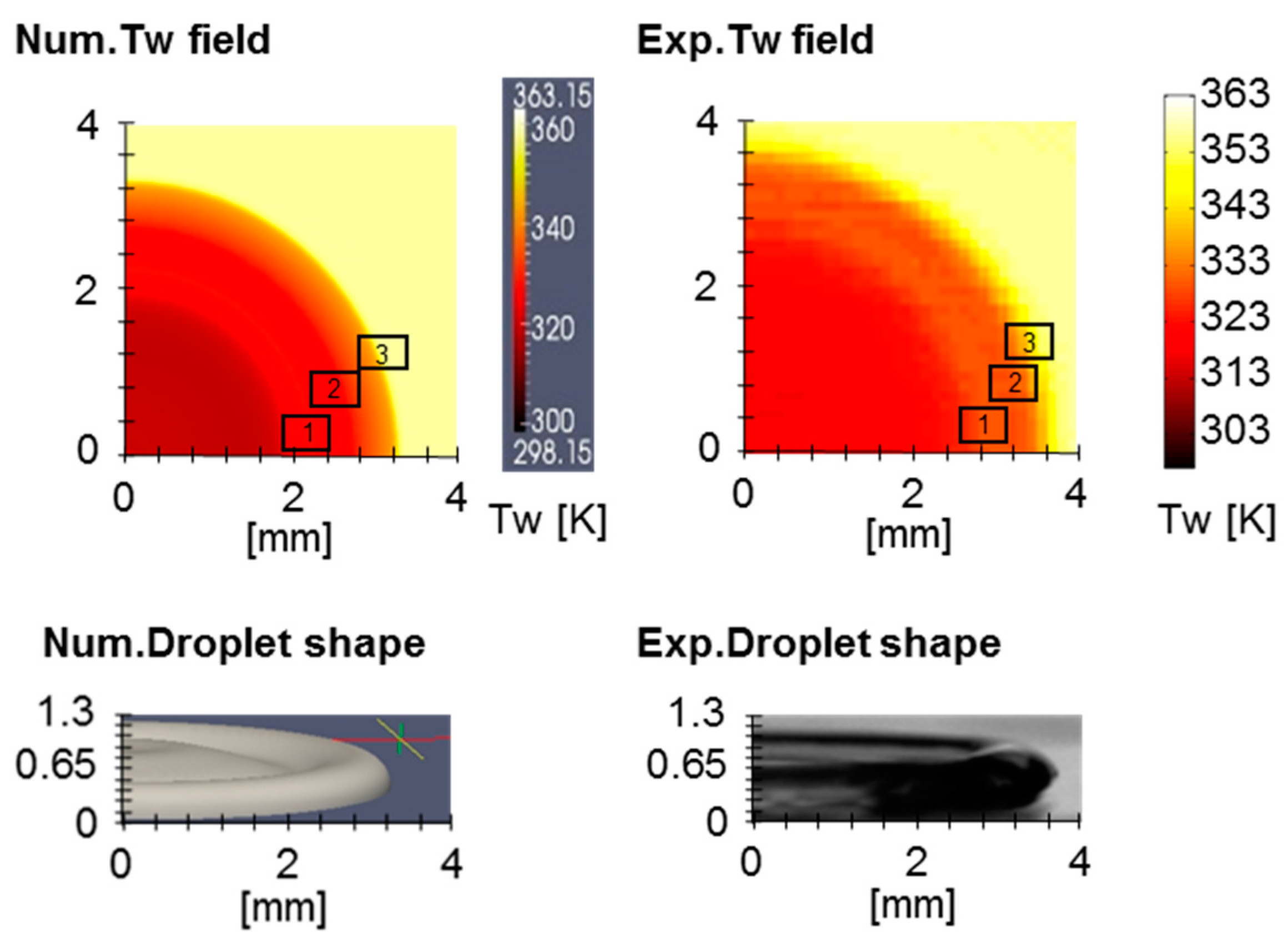
A first qualitative comparison between the experimental results and the corresponding numerical predictions is depicted in Figure 5, for the case of We = 24 (-) and Tw(in) = 353.15 K. In the thermal images, t = 0 ms corresponds to the time of impact identified from the IR images, as the first frame in which a temperature variation was noticed, while in the high-speed images t = 0 ms was identified as the frame in between no contact and evident contact between the droplet and the heating surface was observed.
From a first approximate analysis, it can be inferred that, for all the reported time steps, the numerically predicted droplet shapes and temperature fields at the bottom of the heated foil agree with the experimental data. From the observation of the droplet shape one can notice the typical droplet dynamics during impact and subsequent spreading. The droplet contact diameter increases at higher rate at the first stages of impact, to then stabilize at the last time instances, near the maximum spreading diameter. The height of the droplet bulk decreases along time as the lamella becomes thinner and a rim is generated at the edges of the droplet. At the latter time instances of spreading, the vertical extension of the rim starts to increase due to fluid recirculation towards the droplet centre that feed with new fluid the rim region.
The resulting thermal footprint of the droplet follows the behaviour of the contact diameter along time, in terms of dimensions and is strongly influenced from the droplet dynamics. In fact, the temperature distribution is far from being homogeneous, as one can notice a monotonic decrease of temperature from the centre of the droplet towards the periphery at the first stages of impact (t = 0–2 ms). Moreover, at the late stages of impact (t = 4–6 ms), regions of temperature variation are evident at the edges of the droplet which could be related with the fluid dynamics within the rim as further elucidated in the next paragraphs.
Discrepancies between numerical results and experiments can be revealed from a deeper analysis of Figure 5. At time t = 0 ms, the experimental and calculated surface temperature (Tw) differ mostly in terms of dimensions of the thermal footprint of the droplet. Similarly, in all the consecutive time instants, the measured temperature fields are slightly larger than the numerical ones.
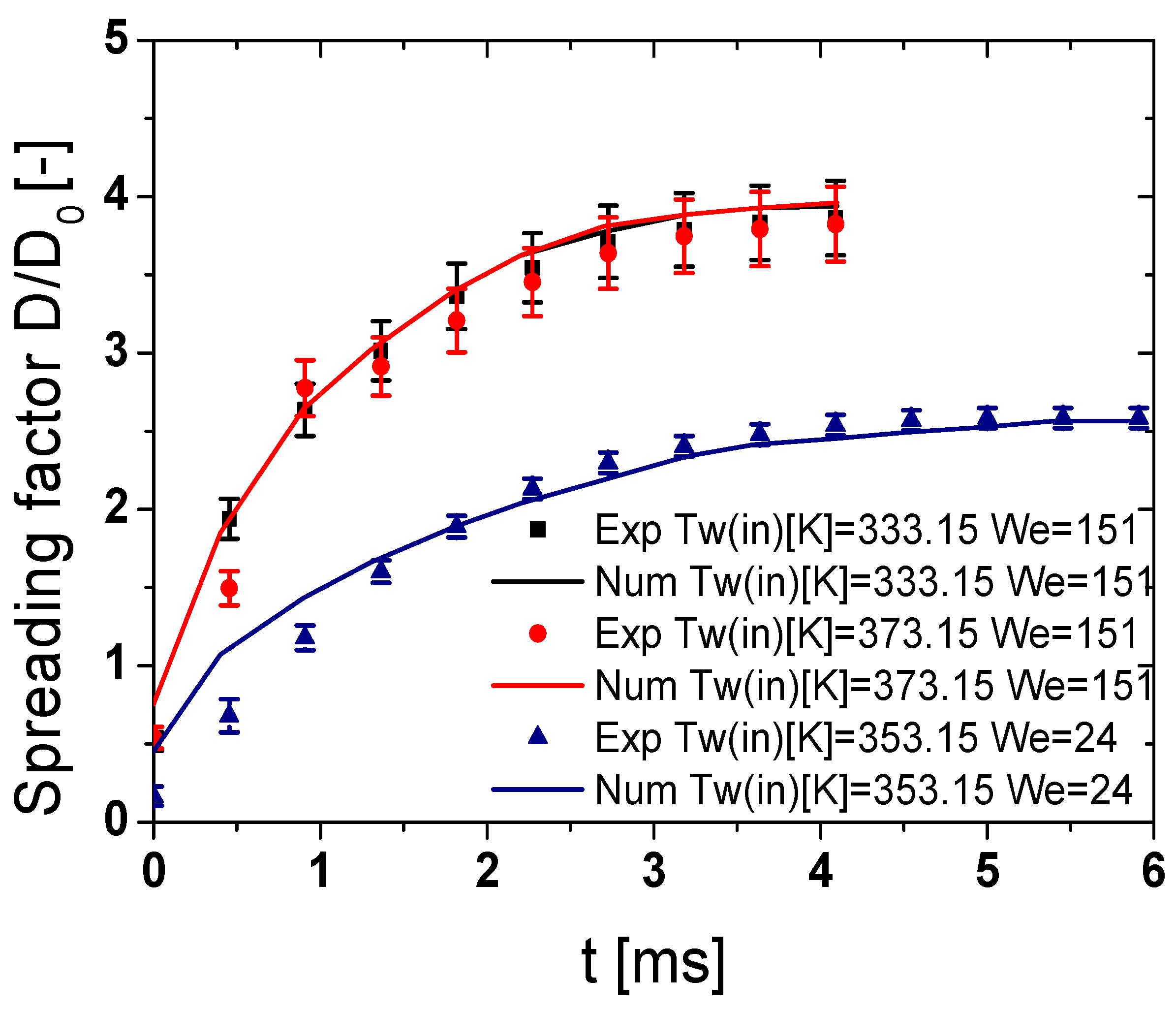
The discussion reported so far referred to test conditions of We = 24, Tw(in) =353.15 K, and comparison between numerical and experimental results has been considered only in qualitative terms. Focusing more in a quantitative analysis, a proper experimental assessment of the contact diameter along time can be performed, and from the latter, the spreading factor can be evaluated. In this context, Figure 6 depicts the temporal evolution of the calculated and measured spreading factors showing that extremely good agreement is found between the numerical and the experimental results. At the first stage of spreading (t < 1 ms) discrepancies are mostly due to the procedure of defining the instant in which impact occurs, as previously reported. In fact, according to the high-speed camera frame rate (2000 fps), the actual impact can occur up to 0.5 ms before or after the frame chosen for the definition of the instant of impact. In the numerical simulation, the time resolution of the post-processed data is 0.1 ms. Thus, particularly at the first stages of the impact, such differences between the numerical and the experimental results are reasonable. However, as the spreading factor increases and therefore the time after impact increases, the difference between numerical and experimental results reduces. Finally, at the maximum spreading the maximum difference between the experimentally measured and the numerically predicted spreading factor is 3.4%. Calculated and measured data confirm that greater impact velocity, i.e., greater Weber number, leads to a larger maximum spreading factor, as also highlighted in previous investigations (e.g., [11]). The higher inertia of the impinging droplet results in a larger spreading diameter.
A significant effect of the initial foil temperature could not be detected, for the same Weber number (We = 151), in the measured spreading factors. In fact, the difference between the maximum spreading factor measured for two different initial foil temperatures, Tw(in) = 373.15 K and Tw(in) = 353.15 K is less than 1%. These findings are in agreement with [8], who concluded that the spreading rate of the droplet is independent of the surface temperature during the early stages of the impact.
The experimentally measured maximum spreading factors are in the range of those reported in literature. For instance, in [36] the authors measured a maximum spreading factor of 2.1 for a water droplet impinging onto a stainless steel surface (equilibrium contact angle 90°) at We = 27 and at ambient temperature of 298 K. While in [34] maximum spreading factors of 3.1 and 4.1 were reported for water droplets impinging onto a stainless steel surface kept at 393.15 K, for We = 114 and 257, respectively. In the case reported here the maximum spreading factors were 2.6 for We = 24 at Tw(in) = 353.15 K and around 3.8 for We = 151 for all the temperatures studied.
In the numerical set-up considered in the present work, the thermo-physical properties of the fluid are not varying with temperature. Hence, no significant effect can be observed in the spreading factor with respect to the initial temperature. In fact, for We = 151 the spreading factors versus time for different Tw(in), are almost identical. Similarly, in [47] the change of thermo-physical properties with temperature was neglected.
On the other hand, in [30] the authors predicted in their model a 10% variation in the spreading factor when the surface temperature was changed, due to the consequent modification of the thermo-physical properties of the fluids with the temperature. However, since, as explained in Section 2.5 the sensitivity analysis performed did not show a relevant variation of the thermo-physical properties with the temperature, for the ranges studied here, and since no significant variation was observed also in the experimental data obtained in the present investigation, due to the increase of the surface temperature, it was decided not to include the variation of the thermo-physical properties with temperature in the numerical simulations.
A first relation can be established between droplet dynamics and heat transfer by direct comparison of the dimensionless surface temperature (T*, Equation (2)) profiles along the dimensionless radial distance at different instants after impact.
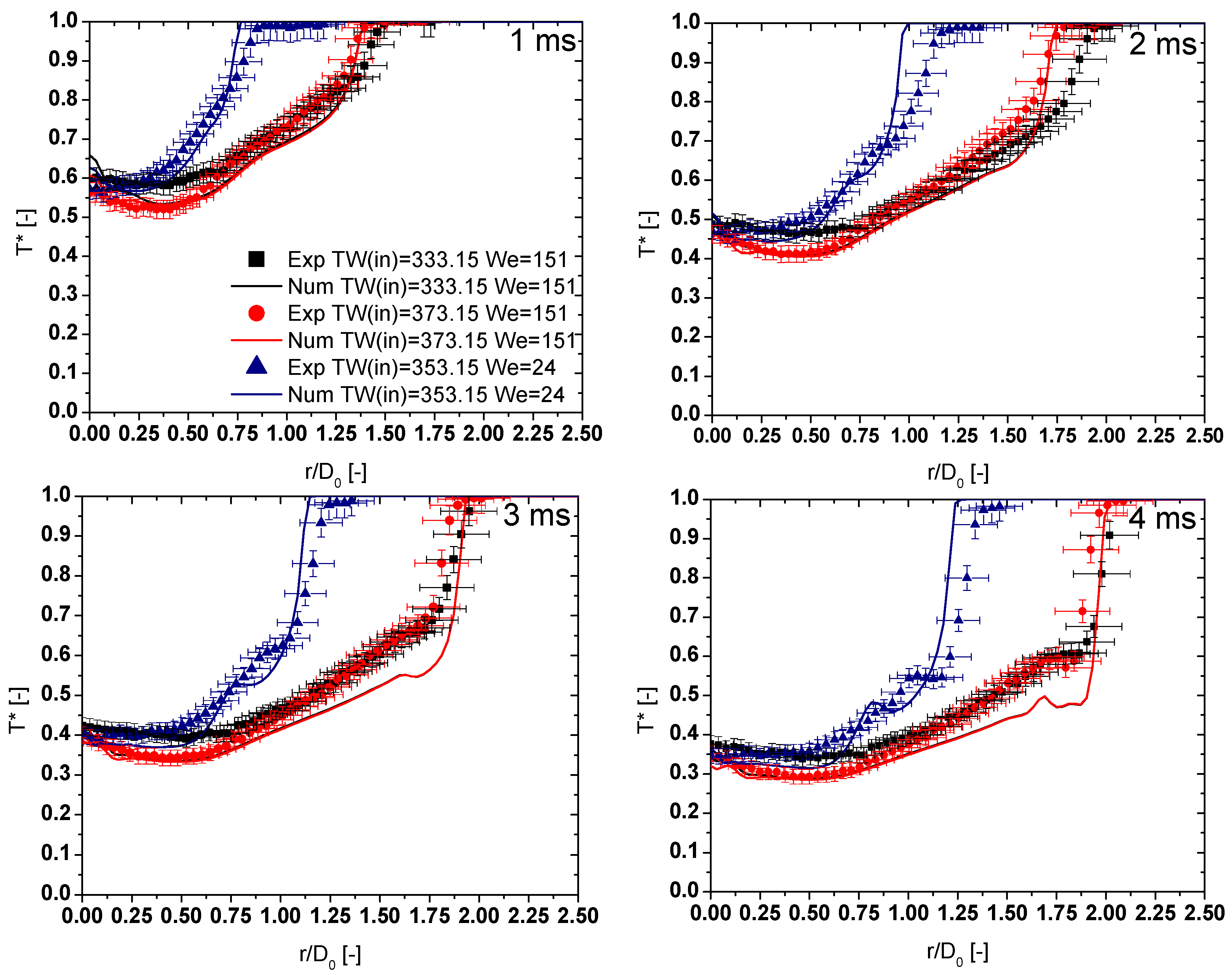
Figure 7, depicts the experimental and the calculated surface dimensionless temperature along the dimensionless radial distance, at different instants after the impact. All the numerically predicted results are reported with a continuous line, while the corresponding experimental results are represented just with symbols. Numerical results at We = 151 are reported in black and red lines. However, since the numerical spreading factor almost overlaps for the same Weber number, in the plots reported in Figure 7 only the red line is more visible. Also, since the maximum spreading diameter for We = 151 is reached 4 ms after impact, the results are only presented and discussed up to this time instant.
The figure cleary shows a very good agreement between the experimental and numerical results, particularly towards the center of the impact region (), for all the conditions tested. For We = 151 in the range or the maximum difference in T* was 11%. For We = 24 in the range the maximum difference in T* was 5%. It should be mentioned here that these differences are comparable with the uncertainty in the experimental measurements.
Some discrepancies are however noticeable at higher values of , at the region of the rim and of the gas-liquid-solid contact line. The contact line can be indetified in terms of position as the maximum before T* = 1. T* = 1 indicates in fact that no temperature variation occurred in the wall and thus the wall is not wetted yet by the droplet. Close to the contact line, a steep temperature variation occurs. Consequently, any small difference between the measured and the calcultated position of the contact line can lead to substantial differences between the measured and the numerically predicted T*, which may reach up to 30% of the experimentally measured value. The rim region is identified by the non monotonic decrease in temperature along . Both experimental and numerical results show that the temperature does not decrease with increasing , but local maxima and minima occur. This is particularly evident in the case of t = 3 and 4 ms after impact, for all the We numbers tested. Here, the maximum difference between the experimental and the numerical values of T* was 16% for We = 151 at 4 ms after impact and at and 11% for We = 24 at 4 ms after impact and at .
Close to the rim, various heat transfer mechanisms occur in extremely small temporal and spatial scales. This implies that matching between the experimental and the numerically calculated temperatures is, on one side strongly dependent on the relation between the instrumental and the numerical resolution and on the other side considerably affected by other physical phenomena such as for example “fingering” at the late stage of spreading (Figure 8). The latter was in fact experimentally observed for higher weber numbers, i.e., We = 151.
Fingering of the lamella, at this stage of the work, could not be reproduced numerically. Since the occurrence of this phenomenon leads to irregular temperature field, especially in the rim region, it can contribute to the discrepancies found between measured and calculated radial temperature profiles at values of . However, a proper quantification of the influence of “fingering” of the lamella on the measured temperature is not addressed here due to its stochastic nature.
Focusing now on the differences in terms of resolution, in the numerical simulations the mesh size varies between 4 µm up to 20 µm and the reported numerical profiles were sampled with a sampling size of 80 µm. Temporal resolution was 0.1 ms. On the other hand, the spatial resolution of the IR camera was of 110 µm/px, the temporal resolution of the IR camera is 1 ms and the integration time was 200 µs. This means that the temperature variation captured by the IR camera could be integrated within a larger temporal-spatial domain and thus the resulting values can be spatially damped or temporal delayed up to a certain amount.
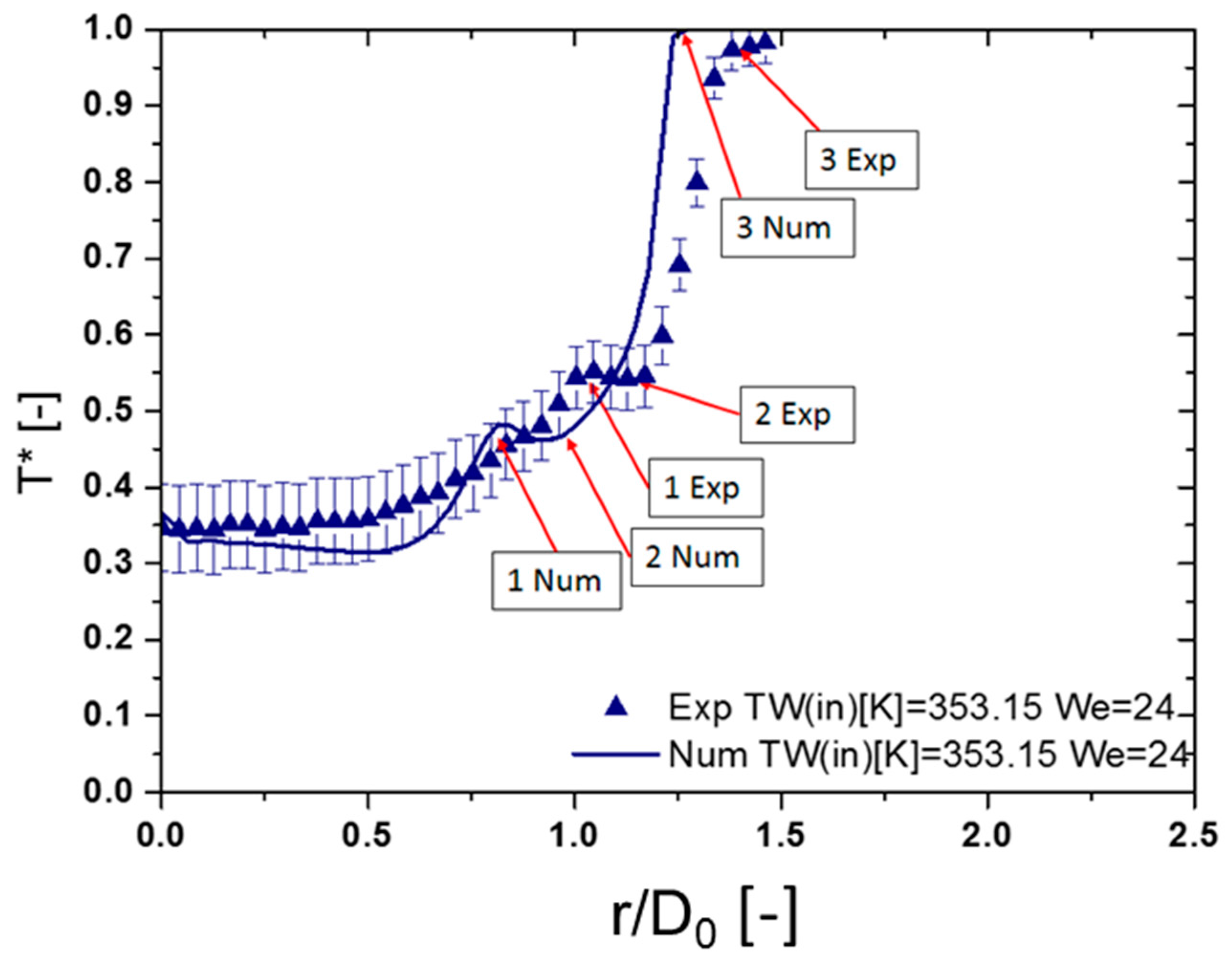
Despite these limitations, the trend of the temperature profiles is well captured by the numerical simulations. This is particularly important in the stages of impact that involve a rim formation. At this stage of impact, three typical characteristic regions can be identified in the temperature profile as reported in Figure 9 and Figure 10. The first is a steep increase in temperature at the entrance to the rim, the second is the appearance of a temperature local minimum in the region within the rim and the third is a steep decrease in temperature that is observed near the contact line. Figure 9 depicts the temperature profile within the rim for the case of We = 24 and Tw(in) = 353.15 K, at 4 ms after the impact. The three typical characteristic regions are identified in the proposed figure by numbered boxes. Number 1, corresponds to the a region just after the entrance of the rim, number 2 identifies the region within the rim and number 3 refers to the contact line. The position of the three characteristic regions is not necessarly in agreement when comparing calculated and measured temperature profiles. In fact, from Figure 8 it can be noticed that the rim entrance (box number 1) in the numerical simulations is observed at values of , while in the experimental case at . The corresponding spatial difference is 0.55 mm. This displacement is then similar for all the other regions identified. However the radial distace between box 1 and 3 resulted to be quite similar, being in the experimental case 0.9 mm, while in the numerical case 1.1 mm.
These regions are also qualitatively identified in Figure 10, which compares the experimentally obtained temperature distribution at the bottom of the heated foil and the high-speed image (to visualize the region of the lamella being addressed) at 4 ms after the impact, with the corresponding numerical prediction.
Experimentally, this description differs from that reported by [21], who measured a constant increase of the temperature along the droplet radius due to the decreased convective heat transfer in the outward fluid direction. Numerically, instead, a temperature distribution similar to that observed here, was also highlighted before in [30,34,35]. In [35] the authors correlated the steep decrease in the temperature at the contact line with the heat removed by evaporation in this region. On the other hand, in [30], the authors related the temperature maxima with the diminished thickness of the lamella just at the entrance of the rim.
In [34], the authors noticed a reverse flow within the droplet which could result in variation of temperature and heat transfer. The discrepancies arising from experimental and numerical studies and the possibility to explain them by correlating the flow field within the droplet and the heat transfer within the solid surface, as suggested by [34], lead the authors of the present investigation to search for a more detailed description of the fluid dynamics within the droplet, specifically at the lamella and within the rim.
3.2. Relation Between Heat Tranfer and Droplet Dynamics
From the analysis presented in the previous subsection, it can be deduced that local variations of temperature, i.e., heat transfer along the radial distance, might be related with the fluid dynamics of the droplet. This relation is more evident in the rim region, where adverse flow can occur, as reported for example in [18] and [34]. The present subsection attempts an accurate description of the correlation between droplet dynamics and heat transfer with emphasis on the rim region, in the case of We = 24 and Tw(in) = 353.15 K. This condition has been selected, since at higher Weber numbers, fingering starts to occur at the edges of the lamella, as captured in the high speed images (see Figure 8).
This phenomenon, as previously mentioned, could not be reproduced by the axisymmetric numerical simulations. A first insight in the fluid dynamics in the rim region and the resulting heat transfer is given in Figure 11 that refers to the fluid region only at 4 ms after impact. The calculated temperature field in the rim region highlights that only a thin layer of fluid is heated during the spreading process. The fluid is colder within the rim, apart from the rim entrance, where hotter fluid can be traced also away from the liquid-solid interface. The radial velocity field presents regions of adverse flow i.e., negative velocity, which are then better identified by the vorticity field, calculated in the Z direction. The Z component of vorticity is chosen since it was considered more characteristic of the flow within the rim that mostly presents velocity variations along the X-Y plane. Here X represents the radial direction. It can be noticed that a complex structure of vortices exists within the rim. In detail, focusing on the region close to the solid wall three different vortex structures can be identified: a clockwise vortex (negative vorticity) just before the entrance to the rim, an anticlockwise vortex (positive vorticity) within the rim and a clockwise vortex (negative vorticity), at the pinned contact line. These vortex structures can influence the transient heat and mass transfer within the bulk fluid and lead to mixing of the thermal boundary layer which is of importance at the liquid-solid interface. Consequently, they should be taken into consideration, especially when dealing with sensible heat transfer. Therefore, it is worth exploring the potential link between the vorticity field and the heat transfer process near the liquid-solid interface.
For this purpose, the vorticity is evaluated and correlated with the heat transfer coefficient at the centre of the first layer of fluid cells i.e., at a vertical distance of 2 µm from the liquid-solid interface.
The vorticity in the Z-direction can be expressed as in Equation (14):
were is the derivative of the radial component of the velocity on y (along the vertical direction). is the derivative of the vertical component of the velocity along the radial direction.
The heat transfer coefficient measured at the first layer of fluid cells can be defined as:
where is the initial droplet temperature (293.15 K) i.e., the ambient temperature imposed before impact, while is the temperature at the wall measured at time t and at a radial distance r from the centre of the impact. is the vertical gradient of the temperature of the fluid and is sampled at the centre of the first layer of fluid cells.
Before analysing the correlation between heat transfer coefficient and vorticity, one should consider the following:
Due to the assumption of axisymmetric geometry, the vorticity becomes a scalar field directed always perpendicularly to the X-Y plane with its signed numerical value identifying the magnitude and direction of the rotational flow.
The components and of the vorticity field were found to be negligible when compared to , consequently only the latter have been considered.
In Equation (14), accounts also for phenomena occurring in the fluid layers on top of the first layer of cells near the wall.
near the liquid-solid interface is usually an order of magnitude lower than .
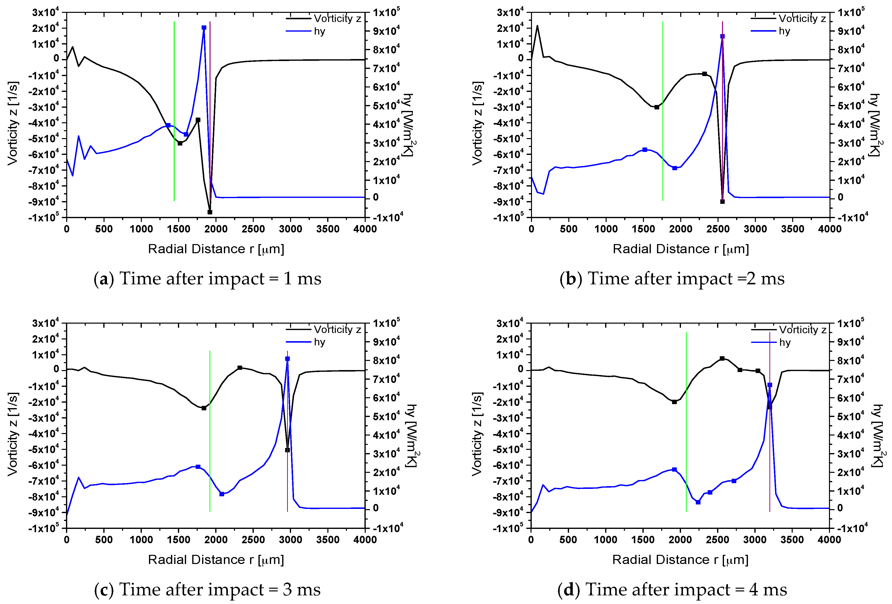
Figure 12, shows the numerically evaluated profiles of Z-vorticity and heat transfer coefficient along the radial distance from the centre of the droplet. Half of the computational domain (i.e., 4000 µm) is considered here to enhance visibility to the results. In the plots, the squares highlight the local maxima or minima of the two compared parameters in the rim region. The position of the rim entrance is depicted by a light green line. The position of the contact line is depicted by a purple line.
From a first analysis, it can be observed that the heat transfer coefficient values evaluated according to the proposed formulation are in the same order of magnitude as those reported in the, literature by [2] and [3] for the sensible heat transfer removed by spray cooling. In the present investigation, a maximum heat transfer coefficient of 91,831 W/m2·K was evaluated at t = 1 ms after the impact and at a radial distance r = 1840 µm. The corresponding minimum value was around 3900 W/m2·K at t = 4 ms after impact and at a radial distance r = 2240 µm.
Still referring to Figure 12, it is possible to observe a correlation between vorticity and heat transfer coefficient in all time instants. In fact, the “trends” of the two parameters with respect to the radial distance from the droplet impact centre are in a way inverted. This is more evident in the wider region of the droplet rim (region between the green and purple line). In more detail, a local maximum in the heat transfer coefficient always corresponds to a local minimum in the vorticity and vice versa. In most of the presented time instants, slightly before the entrance to the rim there is a minimum in the vorticity (negative vorticity), corresponding to a local maximum in the heat transfer coefficient. Only in the case of 1 ms after impact, the proposed minimum in the vorticity is placed a little bit after the entrance to the rim. This can be explained since in this time instance, the rim is not well defined yet. At the contact line a local maximum in the heat transfer coefficient, in all time instances, corresponds to a minimum in the vorticity. The minimum of the vorticity (i.e., negative vorticity) in the contact line is expected due to the passage to zero velocity of the droplet, just after the contact line.
From all the above, it is evident that there is a relationship between local peaks (maxima/minima) in the vorticity and in the heat transfer coefficient, in the regions near the rim, within the rim and at the contact line. However, in most cases a small spatial shift can be observed between the position of the local maxima/minima in the vorticity and the corresponding local minima/maxima in the heat transfer coefficient. This shift can be due to the fact that the vorticity accounts also for the heat and mass transfer within the bulk fluid, so the spatial shift can be seen as a “spatial gap” between the phenomena of heat removal occurring at the liquid/solid interface (represented by the calculated heat transfer coefficients) and those occurring within the bulk rim correlated with the vorticity. However, the complexity of the flow field does not allow at this stage to find a proper correlation between vorticity and heat transfer coefficient. Consequently, in the following subsection, a simplified theoretical formulation is suggested attempting to quantify the observed spatial shift in the local peaks and compare it with the corresponding numerically predicted value.
3.3. Theoretical Analysis of Heat and Mass Tranfer in the Rim Region
Spatial shifts, from now ahead called , between the maxima and the minima of the heat transfer coefficient and vorticity, were noticed in the rim region. In detail, is the distance between the local maximum of the heat transfer coefficient at a radial distance r and the corresponding local minimum of the vorticity at a radial distance . The same definition holds if a local minimum in the heat transfer coefficient is correlated with the corresponding local maximum in the vorticity.
As previously suggested the existence of these shifts can be connected with the different mechanisms of heat and mass transfer occurring at the liquid/solid interface and within the bulk of rim, respectively. In the liquid/solid interface, heat is mainly transported by convection, while within the bulk of the rim, remixing of the thermal boundary layer and transient heat and mass transfer due to vorticity, is believed to be one of the main mechanisms of heat transfer. The latter is influenced by the thermal inertia of the fluid and is more sensible to transient phenomena characterizing droplet spreading.
Taking into account these considerations, the two identified concurring mechanisms of heat transfer can be expressed in a simplified form by the following energy balance for a single cell:
where is the volume of the cell, is the variation of the fluid cell temperature with time, is the temperature of the cell face at the solid/liquid interface. The left-hand side of the equation identifies transient heat removal while the right-hand side identifies heat removed by convection only, in agreement with the two main mechanisms of heat transfer previously highlighted.
The proposed simplified single cell energy balance is only a guideline. In fact, the effect of vorticity should be addressed within the bulk rim. Following this reasoning, Equation (16) can be modified and consequently the heat transported by convection in the first layer of the fluid near the heated foil, can be correlated with the transient heat and mass transport phenomena occurring within the bulk rim using the following proposed formulation:
where on the right-hand side of Equation (17), is the heat removed at the first fluid cell by convection. corresponds to the initial temperature of the droplet.
On the left-hand side accounts for the thermal mass of the rim, is the surface wetted by the droplet, is a characteristic vertical dimension, indicates a typical temperature variation in the fluid occurring in the spatial range of the shift and is a characteristic velocity. The left-hand side of Equation (17) is still correlated with transient phenomena, similarly to the left-hand side of Equation (16). This can be explained, since it includes a characteristic velocity and can now be used for a single time step once the has been introduced. The theoretical shift at this stage allows to study transient phenomena as stationary, by means of the following correlation:
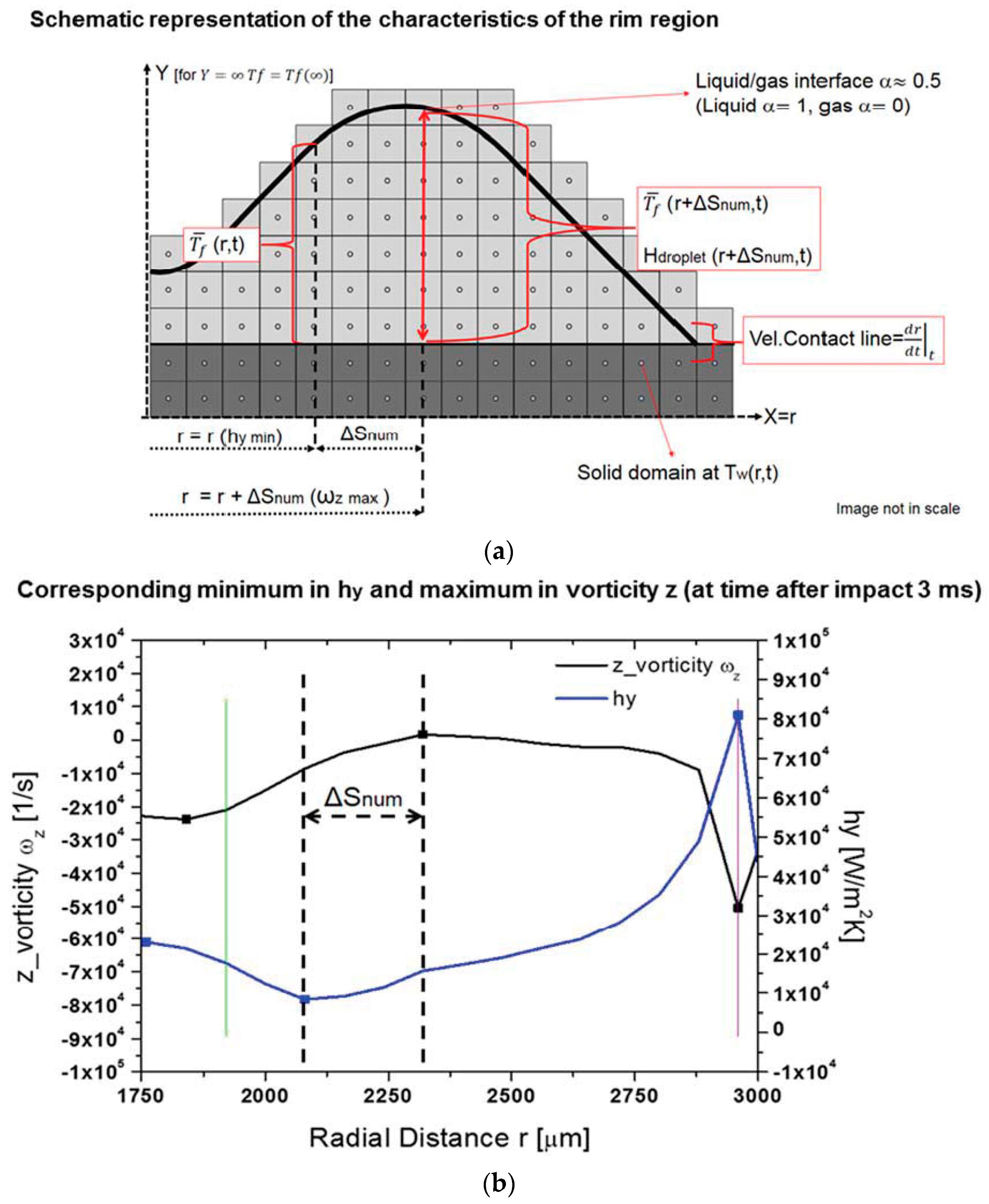
From Equation (17), a theoretical shift can be calculated (), which can then be compared with the one evaluated numerically. For the evaluation of the theoretical shift and in order to properly represent the rim thermo-fluid dynamics, the following assumptions are considered (see Figure 12):
- A characteristic dimension for the vorticity field is the height of the droplet measured at the position of the minima or maxima of the vorticity, . The height of the droplet corresponds to the maximum value of the Y coordinate, measured for a volume fraction of . Therefore, the height of the droplet coincides with the vertical position of the liquid-air interface. substitutes the distance in Equation (17).
- The shifts relate to phenomena occurring in the bulk of the rim. Hence, the variation of the average temperature of the fluid measured along the shift dimension, should be accounted as . Here is the average temperature where the local minima or maxima of the heat transfer coefficient are, while is the average temperature at the corresponding local maxima or minima of the vorticity. The average temperature of the fluid is obtained as the average of the calculated temperatures in the vertical direction of the droplet for . replaces in the initially proposed formulation (Equation (17)).
- A characteristic velocity of the droplet can be defined as measured in time by the forward finite difference method, from the previously obtained spreading factors. This has been chosen since the minima or maxima for the vorticity and heat transfer coefficient in the region of the contact line, move together with the contact line and consequently with a velocity similar to . The proposed velocity also accounts for the bulk conditions of the droplet. This characteristic velocity substitutes in Equation (17).
In summary, since the vorticity is related with phenomena occurring in the bulk of the rim, the initially proposed formulation is accordingly modified to account for variables more related with the bulk properties of the rim.
Figure 13a provides a schematic description of the assumptions for the calculation of the theoretical shift between minimum of heat transfer coefficient and maximum of vorticity observed in the bulk rim, as for example at t = 3 ms after impact (Figure 13b).
Once all the proposed assumptions are considered, the initially proposed formulation is modified as follows:
Rearranging Equation (18), the theoretical shift can be calculated as follows:
As proposed, the confirms to be an instantaneous “spatial gap” between heat and mass transfer within the bulk rim and heat transferred by convection only, in a similar way to the explanation suggested in the previous section.
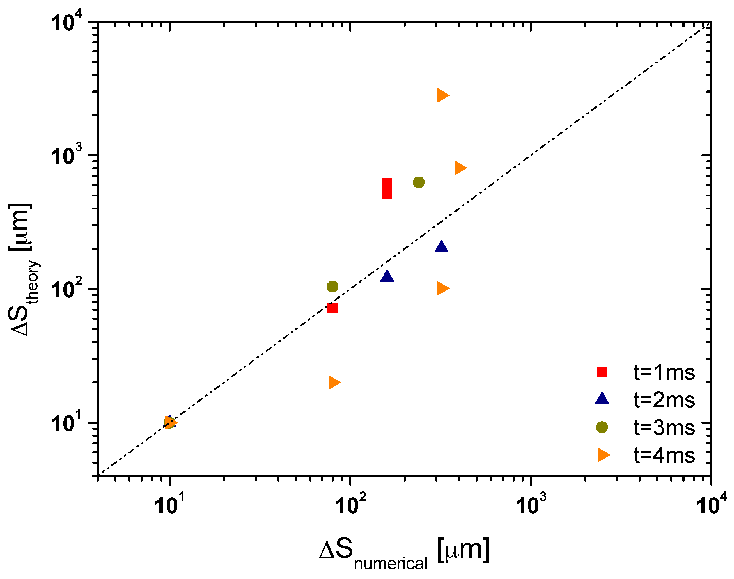
An overview of the variables of interest and of the obtained theoretical shifts for t = 1, 2, 3 and 4 ms after droplet impact, in the case of We = 24 and Tw(in) = 353.15 K is summarized in Table 5. Figure 14 depicts a comparison between numerical and theoretical shifts.
The evaluated theoretical shifts are of the same order of magnitude as the numerical ones in most cases, as shown in Figure 14. The only exception was identified for t = 4 ms after impact, where for a numerical shift of 320 µm, a theoretical shift of 2811 µm was found (see Table 5). This is mostly due to two concurring factors: the increased average temperature of the fluid and the increased height of the liquid in the rim which, according to Equation (17), leads to an overevaluated theoretical shift. Despite this limitation, the proposed formulation is believed to be a proper first attempt to clarify heat and mass transport phenomena, occurring in the rim region. However, since the suggested theoretical formulation is a first approach to the problem and oversimplifies a quite complex mechanism, a further detailed investigation is now required, sustained by wider number of simulations.
4. Conclusions
The spreading process, coupled with the heat transfer process occurring at droplet interaction with a heated surface are studied numerically and experimentally in the present paper. A detailed comparison is performed between the numerically and experimentally obtained droplet spreading factors and surface temperature fields, resulting from the cooling of the droplet impacting onto a thin stainless steel foil (20 μm thick). The numerically obtained spreading factors were in extremely good agreement with the experimental values. The calculated solid surface temperature fields were also in good agreement with those obtained experimentally by high speed IR thermography. The main characteristics of the surface temperature field measured were reproduced properly by the numerical solver. The temperature fields revealed a non-homogenous cooling of the surface, which was correlated with droplet dynamics.
The correlation between the resulted temperature field and droplet dynamics was obtained by assuming a relation between the vorticity and the local heat transfer coefficient, in the first fluid cell i.e., near the liquid-solid interface. The two measured fields revealed that local maxima and minima in the vorticity correspond to spatially shifted local minima and maxima in the heat transfer coefficient, at all stages of droplet spreading. This was particularly clear in the rim region. This is an important new finding that according to the authors’ best knowledge has not been reported in previous similar investigations. Following this analysis, a formulation to theoretically calculate these spatial shifts is proposed. The theoretically calculated shifts were in most of the cases within the same order of magnitude with the corresponding numerically predicted values. However, additional simulations must be performed in the future, to further improve this preliminary formulation.
In summary, the present investigation adds significantly to the existing knowledge of sensible heat transfer during droplet cooling. Finally, it can be said that the use of the improved VOF-based interface-capturing approach, which was proposed, presented, validated and applied in the present investigation, constitutes a quite promising tool for future further investigation in the proposed field.
Acknowledgments
The authors are grateful to Fundação para a Ciência e Tecnologia (FCT) for partially financing the research under the framework of the project RECI/EMS-SIS/0147/2012 and for supporting Pedro Pontes with a research fellowship. Ana Moita acknowledges FCT for financing her contract through the IF 2015 recruitment program (IF 00810-2015) and Emanuele Teodori acknowledges FCT for supporting his PhD fellowship (SFRH/BD/88102/2012). Finally, the authors are grateful to Y. Liu from Jilin University, for providing the thin stainless steel foils used in the experimental tests.
Author Contributions
Emanuele Teodori contributed to the development of the conjugate heat transfer solver. In detail, he modified the existing VOF code to account for conjugate heat transfer between fluid and solid domains. He performed and set the simulations and he compared the numerical results with the experimental results. He designed the experimental procedure to be followed, and he partially designed and assembled the heating assembly. He performed the evaluation of all the uncertainties related with the measured values and wrote the first draft of the paper. Pedro Pontes, improved the firstly devised heating assembly, performed the experiments, re-calibrated the IR camera and developed a Matlab code to post process the IR images. Ana Moita contributed in the discussion of the results of droplet spreading particularly in the experimental part. Moreover, she supervised the activities performed by Pedro Pontes. Anastasios Georgoulas and Marco Marengo have developed in the past the enhanced VOF solver that formed the basis of the present numerical activities. Furthermore, they contributed in the training of Emanuele Teodori in the use and interaction with the proposed VOF code and they supervised the overall numerical activities. Antonio Moreira, supervised the overall experimental activities performed by Emanuele Teodori. All authors contributed equally in the analysis of the overall data, the writing and revision of the present paper.
Conflicts of Interest
The authors declare no conflict of interest.
References
- Kim, J. Spray cooling heat transfer: The state of the art. Int. J. Heat Fluid Flow 2007, 28, 753–767. [Google Scholar] [CrossRef]
- Karwa, N.; Kale, S.R.; Subbarao, P.M.V. Experimental study of non-boiling heat transfer from a horizontal surface by water sprays. Exp. Therm. Fluid Sci. 2007, 32, 571–579. [Google Scholar] [CrossRef]
- Wang, Y.; Liu, M.; Liu, D.; Xu, K. Heat flux correlation for spray cooling in the nonboiling regime. Heat Transf. Eng. 2011, 32, 1075–1081. [Google Scholar] [CrossRef]
- Rein, M. Phenomena of liquid drop impact on solid and liquid surfaces. Fluid Dyn. Res. 1993, 12, 61–93. [Google Scholar] [CrossRef]
- Yarin, A.L. Drop impact dynamics: Splashing, spreading, receding, bouncing. Annu. Rev. Fluid Mech. 2005, 38, 159–192. [Google Scholar] [CrossRef]
- Josserand, C.; Thoroddsen, S.T. Drop impact on a solid surface. Annu. Rev. Fluid Mech. 2016, 48, 365–391. [Google Scholar] [CrossRef]
- Moreira, A.L.N.; Moita, A.S.; Panão, M.R. Advances and challenges in explaining fuel spray impingement: How much of single droplet impact research is useful? Prog. Energy Combust. Sci. 2010, 36, 554–580. [Google Scholar] [CrossRef]
- Chandra, S.; Avedisian, C.T. On the collision of a droplet with a solid surface. Proc. R. Soc. Lond. Ser. A Math. Phys. Sci. 1991, 432, 1525. [Google Scholar] [CrossRef]
- Antonini, C.; Innocenti, M.; Horn, T.; Marengo, M.; Amirfazli, A. Understanding the effect of superhydrophobic coatings on energy reduction in anti-icing systems. Cold Reg. Sci. Technol. 2011, 67, 58–67. [Google Scholar] [CrossRef]
- Moita, A.S.; Moreira, A.L.N. Drop impacts onto cold and heated rigid surfaces: Morphological comparisons, disintegration limits and secondary atomization. Int. J. Heat Fluid Flow 2007, 28, 735–752. [Google Scholar] [CrossRef]
- Rioboo, R.; Marengo, M.; Tropea, C. Time evolution of liquid drop impact onto solid, dry surfaces. Exp. Fluids 2002, 33, 112–124. [Google Scholar] [CrossRef]
- Moita, A.S.; Moreira, A.L. Experimental study on fuel drop impacts onto rigid surfaces: Morphological comparisons, disintegration limits and secondary atomization. Proc. Combust. Inst. 2007, 31, 2175–2183. [Google Scholar] [CrossRef]
- Liang, G.; Mudawar, I. Review of drop impact on heated walls. Int. J. Heat Mass Transf. 2017, 106, 103–126. [Google Scholar] [CrossRef]
- Lee, J.; Kim, J.; Kiger, K.T. Time- and space-resolved heat transfer characteristics of single droplet cooling using microscale heater arrays. Int. J. Heat Fluid Flow 2001, 22, 188–200. [Google Scholar] [CrossRef]
- Paik, S.W.; Kihm, K.D.; Lee, S.P.; Pratt, D.M. Spatially and temporally resolved temperature measurements for slow evaporating sessile drops heated by a microfabricated heater array. J. Heat Transf. 2006, 129, 966–976. [Google Scholar] [CrossRef]
- Sodtke, C.; Ajaev, V.S.; Stephan, P. Evaporation of thin liquid droplets on heated surfaces. Heat Mass Transf. 2007, 43, 649–657. [Google Scholar] [CrossRef]
- Chen, Q.; Li, Y.; Longtin, J.P. Real-time laser-based measurement of interface temperature during droplet impingement on a cold surface. Int. J. Heat Mass Transf. 2003, 46, 879–888. [Google Scholar] [CrossRef]
- Bhardwaj, R.; Longtin, J.P.; Attinger, D. Interfacial temperature measurements, high-speed visualization and finite-element simulations of droplet impact and evaporation on a solid surface. Int. J. Heat Mass Transf. 2010, 53, 3733–3744. [Google Scholar] [CrossRef]
- Girard, F.; Antoni, M.; Sefiane, K. Infrared thermography investigation of an evaporating sessile water droplet on heated substrates. Langmuir 2010, 26, 4576–4580. [Google Scholar] [CrossRef] [PubMed]
- Tartarini, P.; Corticelli, M.A.; Tarozzi, L. Dropwise cooling: Experimental tests by infrared thermography and numerical simulations. Appl. Therm. Eng. 2009, 29, 1391–1397. [Google Scholar] [CrossRef]
- Jackson, R.G.; Kahani, M.; Karwa, N.; Wu, A.; Lamb, R.; Taylor, R.; Rosengarten, G. Effect of surface wettability on carbon nanotube water-based nanofluid droplet impingement heat transfer. J. Phys. Conf. Ser. 2014, 525, 12024. [Google Scholar] [CrossRef]
- Gradeck, M.; Seiler, N.; Ruyer, P.; Maillet, D. Heat transfer for Leidenfrost drops bouncing onto a hot surface. Exp. Therm. Fluid Sci. 2013, 47, 14–25. [Google Scholar] [CrossRef]
- Gambaryan-Roisman, T.; Budakli, M.; Roisman, I.V.; Stephan, P. Heat transfer during drop impact onto wetted heated smooth and structured substrates: Experimental and theoretical study. Prooceedings of the 14th International Heat Transfer Conference, Washington, DC, USA, 8–13 August 2010; pp. 755–761. [Google Scholar]
- Harlow, F.H.; Shannon, J.P. The splash of a liquid drop. J. Appl. Phys. 1967, 38, 3855–3866. [Google Scholar] [CrossRef]
- Tsurutani, K.; Yao, M.; Senda, J.; Fujimoto, H. Numerical analysis of the deformation process of a droplet impinging upon a wall. JSME Int. J. Ser. 2 Fluids Eng. Heat Transf. Power Combust. Thermophys. Prop. 1990, 33, 555–561. [Google Scholar] [CrossRef]
- Watanabe, T.; Kuribayashi, I.; Honda, T.; Kanzawa, A. Deformation and solidification of a droplet on a cold substrate. Chem. Eng. Sci. 1992, 47, 3059–3065. [Google Scholar] [CrossRef]
- Zhao, Z.; Poulikakos, D.; Fukai, J. Heat transfer and fluid dynamics during the collision of a liquid droplet on a substrate—I. Modeling. Int. J. Heat Mass Transf. 1996, 39, 2771–2789. [Google Scholar] [CrossRef]
- Francois, M.; Shyy, W. Computations of drop dynamics with the immersed boundary method, part 1: Numerical algorithm and buoyancy-induced effect. Numer. Heat Transf. Part B Fundam. 2003, 44, 101–118. [Google Scholar] [CrossRef]
- Francois, M.; Shyy, W. Computations of drop dynamics with the immersed boundary method, part 2: Drop impact and heat transfer. Numer. Heat Transf. Part B Fundam. 2003, 44, 119–143. [Google Scholar] [CrossRef]
- Healy, W.M.; Hartley, J.G.; Abdel-Khalik, S.I. On the validity of the adiabatic spreading assumption in droplet impact cooling. Int. J. Heat Mass Transf. 2001, 44, 3869–3881. [Google Scholar] [CrossRef]
- Rueda Villegas, L.; Tanguy, S.; Castanet, G.; Caballina, O.; Lemoine, F. Direct numerical simulation of the impact of a droplet onto a hot surface above the Leidenfrost temperature. Int. J. Heat Mass Transf. 2017, 104, 1090–1109. [Google Scholar] [CrossRef]
- Attané, P.; Girard, F.; Morin, V. An energy balance approach of the dynamics of drop impact on a solid surface. Phys. Fluids 2007, 19, 12101. [Google Scholar] [CrossRef]
- Roisman, I.V.; Rioboo, R.; Tropea, C. Normal impact of a liquid drop on a dry surface: Model for spreading and receding. Proc. R. Soc. A Math. Phys. Eng. Sci. 2002, 458, 1411–1430. [Google Scholar] [CrossRef]
- Pasandideh-Fard, M.; Aziz, S.D.; Chandra, S.; Mostaghimi, J. Cooling effectiveness of a water drop impinging on a hot surface. Int. J. Heat Fluid Flow 2001, 22, 201–210. [Google Scholar] [CrossRef]
- Strotos, G.; Aleksis, G.; Gavaises, M.; Nikas, K.-S.; Nikolopoulos, N.; Theodorakakos, A. Non-dimensionalisation parameters for predicting the cooling effectiveness of droplets impinging on moderate temperature solid surfaces. Int. J. Therm. Sci. 2011, 50, 698–711. [Google Scholar] [CrossRef]
- Pasandideh-Fard, M.Y.M.; Qiao, Y.M.; Chandra, S.; Mostaghimi, J. Capillary effects during droplet impact on a solid surface. Phys. Fluids 1996, 8, 650–659. [Google Scholar] [CrossRef]
- Vignes-Adler, M. Physico-chemical aspects of forced wetting. In Drop-Surface Interactions; Rein, M., Ed.; Springer: Vienna, Austria, 2002; pp. 103–157. [Google Scholar]
- Marmur, A. Measures of wettability of solid surfaces. Eur. Phys. J. Spec. Top. 2011, 197, 193. [Google Scholar] [CrossRef]
- Rioboo, R. Impactes De Gouttes Sur Surfaces Solides et Sèches. Ph.D. Thesis, Université de Paris VI, Paris, France, 2001. (In French). [Google Scholar]
- Teodori, E.; Valente, T.; Malavasi, I.; Moita, A.S.; Marengo, M.; Moreira, A.L.N. Effect of extreme wetting scenarios on pool boiling conditions. Appl. Therm. Eng. 2016, 115, 1424–1437. [Google Scholar] [CrossRef]
- Georgoulas, A.; Koukouvinis, P.; Gavaises, M.; Marengo, M. Numerical investigation of quasi-static bubble growth and detachment from submerged orifices in isothermal liquid pools: The effect of varying fluid properties and gravity levels. Int. J. Multiph. Flow 2015, 74, 59–78. [Google Scholar] [CrossRef]
- Hoang, D.A.; van Steijn, V.; Portela, L.M.; Kreutzer, M.T.; Kleijn, C.R. Benchmark numerical simulations of segmented two-phase flows in microchannels using the Volume of Fluid method. Comput. Fluids 2013, 86, 28–36. [Google Scholar] [CrossRef]
- Deshpande, S.S.; Anumolu, L.; Trujillo, M.F. Evaluating the performance of the two-phase flow solver interFoam. Comput. Sci. Discov. 2012, 5, 14016. [Google Scholar] [CrossRef]
- OpenFOAM, the Open Source CFD Toolbox, User Guide. Available online: http://www.openfoam.com/documentation/user-guide/ (accessed on 5 June 2017).
- Brackbill, J.; Kothe, D.; Zemach, C. A continuum method for modeling surface tension. J. Comput. Phys. 1992, 100, 335–354. [Google Scholar] [CrossRef]
- Kunkelmann, C. Numerical Modeling and Investigation of Boiling Phenomena. Ph.D. Thesis, Technische Universität, Darmstadt, Germany, 2011. [Google Scholar]
- Healy, W.M.; Hartley, J.G.; Abdel-Khalik, S.I. Comparison between theoretical models and experimental data for the spreading of liquid droplets impacting a solid surface. Int. J. Heat Mass Transf. 1996, 39, 3079–3082. [Google Scholar] [CrossRef]
Figure 1.
(a) Schematic view and (b) photograph of the experimental set up used in the present work.
Figure 1.
(a) Schematic view and (b) photograph of the experimental set up used in the present work.
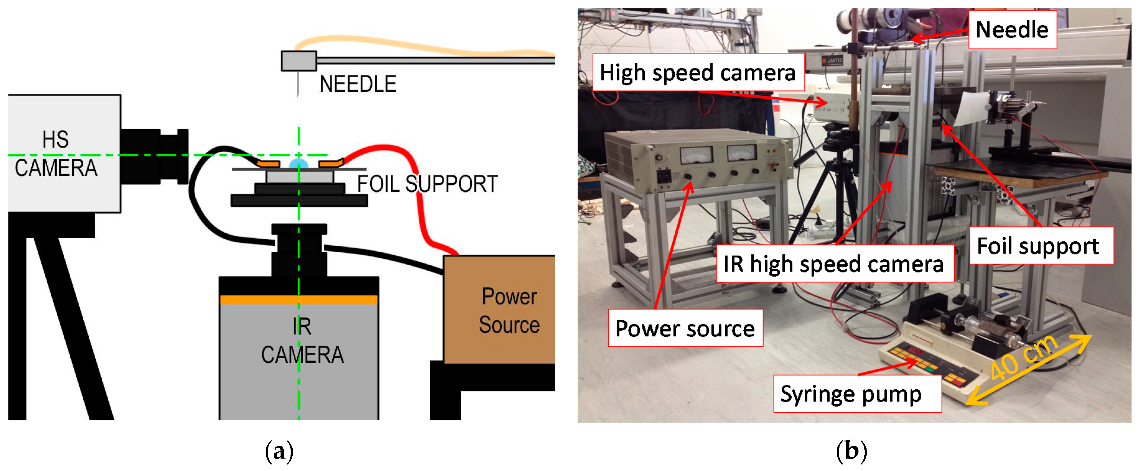
Figure 2.
(a) Detail of the stainless-steel foil and relative position of the IR camera; (b) Foil support and heating assembly.
Figure 2.
(a) Detail of the stainless-steel foil and relative position of the IR camera; (b) Foil support and heating assembly.

Figure 3.
Illustrative representation of a raw and post-processed high-speed image (a). Corresponding infrared thermography and relative temperature profile along the radial direction (b). The blue line in the infrared thermography indicates the radius along which the temperature is measured. The green curve in the post-processed high-speed image, indicates the definition of the interface of the droplet.

Figure 4.
Schematic view of the computational domain, boundary conditions and initial condition for the simulations.
Figure 4.
Schematic view of the computational domain, boundary conditions and initial condition for the simulations.

Figure 5.
Qualitative comparison between high-speed recorded and numerically predicted droplet shape and between experimentally measured and numerically calculated temperature field (Tw) at the bottom of the solid sample. Comparison is presented for different time instants after impact at test conditions We = 24, Tw(in) = 353.15 K.
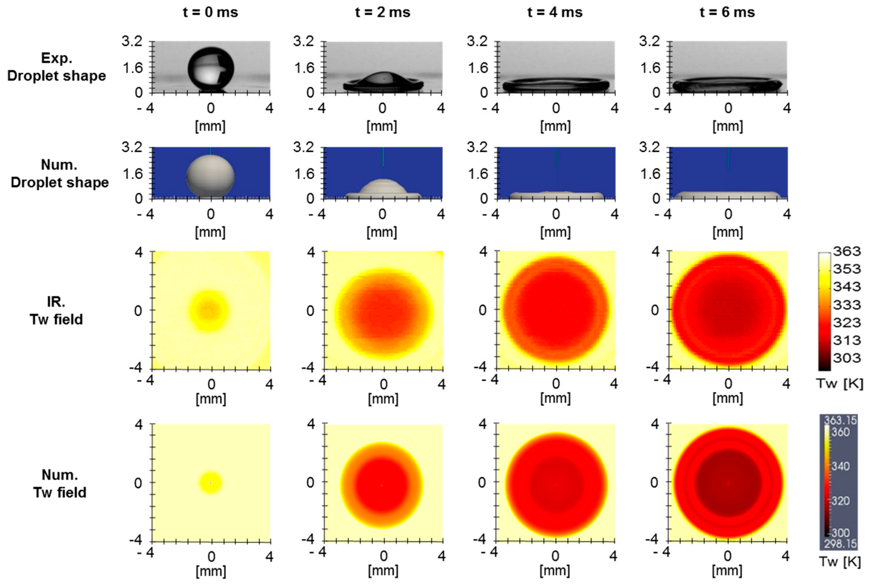
Figure 6.
Evolution of the spreading factor versus time for all the experimental and the corresponding numerical tests performed.
Figure 6.
Evolution of the spreading factor versus time for all the experimental and the corresponding numerical tests performed.

Figure 7.
Distribution of dimensionless temperature within the solid domain, along the dimensionless radial distance for 1, 2, 3 and 4 ms after impact, for all the calculated and measured conditions.
Figure 7.
Distribution of dimensionless temperature within the solid domain, along the dimensionless radial distance for 1, 2, 3 and 4 ms after impact, for all the calculated and measured conditions.

Figure 8.
Example of lamella fingering as captured in the high speed recorded images and in the correspondent IR thermography images, taken from the bottom of the heated stainless steel foil. The blue circle highlights the region where fingering is observed. The reported images refer to We = 151, Tw(in) = 333.15 K and were taken at a time after impact t = 4 ms.
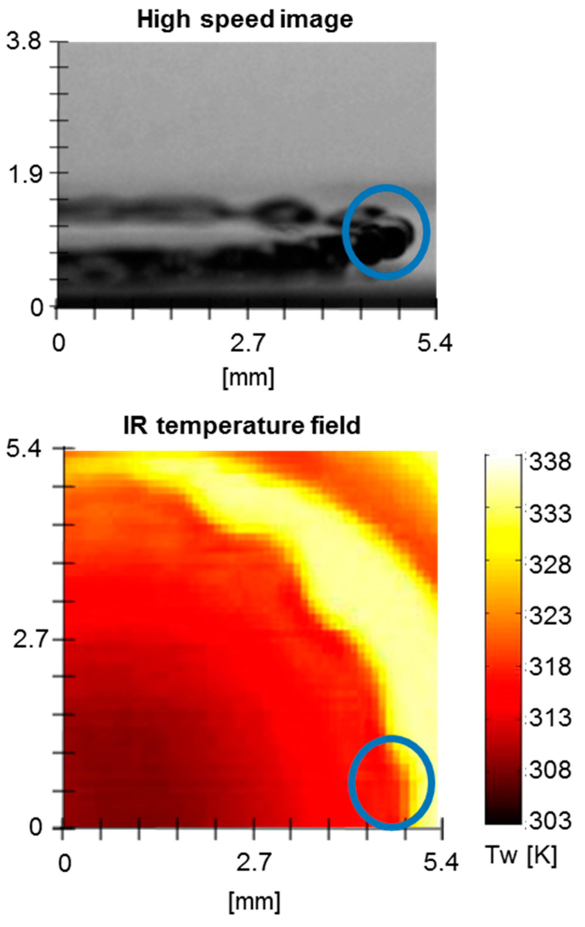
Figure 9.
Measured and calculated temperature distribution along the dimensioless radial distance (We = 24, Tw(in) = 353.15 K).
Figure 9.
Measured and calculated temperature distribution along the dimensioless radial distance (We = 24, Tw(in) = 353.15 K).

Figure 10.
Details of the temperature distribution in the rim region as predicted by the numerical simulation and measured from the IR image (top). Spreading stage of the droplet from corresponding high speed image.
Figure 10.
Details of the temperature distribution in the rim region as predicted by the numerical simulation and measured from the IR image (top). Spreading stage of the droplet from corresponding high speed image.

Figure 11.
Numerically obtained temperature, radial velocity and z-vorticity fields within the fluid domain in the rim region. For We = 24 and Tw(in) = 353.15 K at 4 ms after impact. The z-axis is perpendicular to the plane of view. The white line identifies interface between the liquid and gas phases (alpha = 0.5).
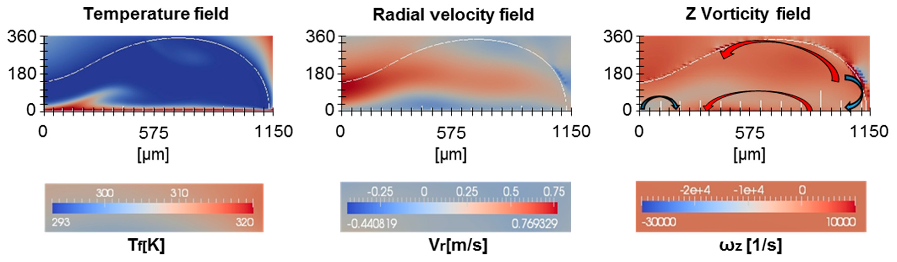
Figure 12.
Vorticity in the Z direction and heat transfer coefficient numerically evaluated along the droplet radial distance, at different times after impact, for We = 24 and Tw(in) = 353.15 K. In the plots, the squares in the curves highlight the local maxima and minima of the numerically evaluated vorticity and heat transfer coefficients. The green line identifies the rim entrance and the purple line identifies the contact line.

Figure 13.
(a) Schematic view of the rim region and representation of the parameters chosen for the final formulation of the theoretical spatial shift between local maxima and minima of heat transfer coefficient and vorticity. The bright grey area represents the fluid domain and the dark grey area the solid domain; (b) Corresponding local minimum in heat transfer coefficient and local maximum in vorticity for which the theoretical shift is calculated.

Figure 14.
Theoretical versus numerical shifts for time after impact t = 1, 2, 3, 4 ms.

Table 1.
Uncertainties of the measured parameters used for heat transfer characterization.
| Parameter | Uncertainties (rel. or abs) | Evaluation Method |
|---|---|---|
| Temperature T (K) | for is the one given by manufacturer. for is calculated after black body recalibration of the Infrared Camera. No standard deviation was accounted. | |
| Temperature difference ΔT (K) | ; ; | ; |
| Non-dimensional temperature T* (-) | ; ; | ; |
| Imposed volumetric heat rate | ||
| Radial distance r (mm) (infrared) | is evaluated according to the resolution in the arrangement used in the study |
Table 2.
Uncertainties of the measured parameters used for the droplet dynamic characterization
| Parameter | Uncertainties (rel. or abs) | Evaluation Method |
|---|---|---|
| Contact Diameter Droplet diameter before impact | The uncertainty of post processed and was given as the maximum uncertainty of the image post processing in the definition of the interface of the droplet. | |
| Spreading ratio (-) | ||
| Impact velocity | In which is the measured value of velocity considering a vertical displacement of the droplet in the time interval between three consecutive frames i.e., 1.5 ms. is the velocity that would result from a displacement equal to in the same interval between three consecutive frames. is considered to be ±1 pixel (40 µm) in the optical arrangement used. | |
| Weber number We (-) |
Table 3.
Thermo-physical properties of the fluids and solid used in the performed simulations.
| Material Properties | (kg/m3) | (J/kg·K) | (W/m·K) | ν (m2/s) | σ (N/m) |
|---|---|---|---|---|---|
| Air | 1 | 1006.4 | 0.025874 | 0.0000148 | - |
| Water | 1000 | 4184 | 0.59844 | 0.000001 | 0.007 |
| Stainless steel | 7880 | 477 | 18 | - | - |
indicates the density, the specific heat, the thermal conductivity, ν the viscosity, σ the surface tension .
Table 4.
Parameters of the conducted simulations.
| (W/m3) | Tw(in) (K) | We (-) |
|---|---|---|
| 98.6 × 10⁶ | 353.15 | 24 |
| 65.4 × 10⁶ | 333.15 | 151 |
| 122.8 × 10⁶ | 373.15 | 151 |
Table 5.
Variables of interest and numerical versus theoretical shifts for We = 24 and Tw(in) = 353.15 K taken at 1, 2, 3 and 4 ms after droplet impact.
Table 5.
Variables of interest and numerical versus theoretical shifts for We = 24 and Tw(in) = 353.15 K taken at 1, 2, 3 and 4 ms after droplet impact.
| Time after Impact = 1 ms | ||||
| 160 | 516 | 238 | 1.3 | 0.67 |
| 160 | 616 | 179 | 2 | 0.67 |
| 80 | 72 | 89 | 1.5 | 0.67 |
| Time after Impact = 2 ms | ||||
| 160 | 121 | 240 | 0.2 | 0.45 |
| 320 | 202 | 298 | 0.3 | 0.45 |
| 0 | 0 | 29 | 0 | 0.45 |
| Time after Impact = 3 ms | ||||
| 80 | 104 | 209 | 0.3 | 0.26 |
| 240 | 626 | 327 | 0.5 | 0.26 |
| 0 | 0 | ≈0 | 0 | 0.26 |
| Time after Impact = 4 ms | ||||
| 80 | 20 | 149 | 0.2 | 0.08 |
| 320 | 2811 | 327 | 3 | 0.08 |
| 400 | 806 | 358 | 3.2 | 0.08 |
| 320 | 101 | 120 | 1.2 | 0.08 |
| 0 | 0 | 0 | 0 | 0.08 |
© 2017 by the authors. Licensee MDPI, Basel, Switzerland. This article is an open access article distributed under the terms and conditions of the Creative Commons Attribution (CC BY) license (http://creativecommons.org/licenses/by/4.0/).
Share and Cite
MDPI and ACS Style
Teodori, E.; Pontes, P.; Moita, A.; Georgoulas, A.; Marengo, M.; Moreira, A. Sensible Heat Transfer during Droplet Cooling: Experimental and Numerical Analysis. Energies 2017, 10, 790. https://doi.org/10.3390/en10060790
AMA Style
Teodori E, Pontes P, Moita A, Georgoulas A, Marengo M, Moreira A. Sensible Heat Transfer during Droplet Cooling: Experimental and Numerical Analysis. Energies. 2017; 10(6):790. https://doi.org/10.3390/en10060790
Chicago/Turabian StyleTeodori, Emanuele, Pedro Pontes, Ana Moita, Anastasios Georgoulas, Marco Marengo, and Antonio Moreira. 2017. "Sensible Heat Transfer during Droplet Cooling: Experimental and Numerical Analysis" Energies 10, no. 6: 790. https://doi.org/10.3390/en10060790
Note that from the first issue of 2016, this journal uses article numbers instead of page numbers. See further details here.