
A Novel Hybrid Model Based on Extreme Learning Machine, k-Nearest Neighbor Regression and Wavelet Denoising Applied to Short-Term Electric Load Forecasting


School of Mathematics and Statistics, Lanzhou University, Lanzhou 730000, Gansu, China
*
Author to whom correspondence should be addressed.
Energies 2017, 10(5), 694; https://doi.org/10.3390/en10050694
Submission received: 24 March 2017
/
Revised: 23 April 2017
/
Accepted: 9 May 2017
/
Published: 16 May 2017
(This article belongs to the Section F: Electrical Engineering)
Abstract
:Electric load forecasting plays an important role in electricity markets and power systems. Because electric load time series are complicated and nonlinear, it is very difficult to achieve a satisfactory forecasting accuracy. In this paper, a hybrid model, Wavelet Denoising-Extreme Learning Machine optimized by k-Nearest Neighbor Regression (EWKM), which combines k-Nearest Neighbor (KNN) and Extreme Learning Machine (ELM) based on a wavelet denoising technique is proposed for short-term load forecasting. The proposed hybrid model decomposes the time series into a low frequency-associated main signal and some detailed signals associated with high frequencies at first, then uses KNN to determine the independent and dependent variables from the low-frequency signal. Finally, the ELM is used to get the non-linear relationship between these variables to get the final prediction result for the electric load. Compared with three other models, Extreme Learning Machine optimized by k-Nearest Neighbor Regression (EKM), Wavelet Denoising-Extreme Learning Machine (WKM) and Wavelet Denoising-Back Propagation Neural Network optimized by k-Nearest Neighbor Regression (WNNM), the model proposed in this paper can improve the accuracy efficiently. New South Wales is the economic powerhouse of Australia, so we use the proposed model to predict electric demand for that region. The accurate prediction has a significant meaning.
Highlights:
- A novel hybrid model named ELM-WA-KNN is proposed for electric load forecasting in New South Wales, Australia.
- The wavelet analysis (WA) is introduced to eliminate the noise of the electric load time series.
- k-Nearest Neighbor regression (KNN) is used to get the input-output relationship in the hybrid model.
- The kernel function of KNN is established by extreme learning machine (ELM).
- The proposed ELM-WA-KNN model has the best performance among all the considered models.
1. Introduction
Electric load prediction is one of the major tasks in power management departments which carry out electric power dispatching, usage and planning. Improving the accuracy of load forecasting is helpful for planning power management and is advantageous to the arrangement of power grid operations. Meanwhile, it is also advantageous for the reduction of power generation costs and is beneficial to establish the power for construction plans. Therefore, electric load forecasting has become an important part of power system management modernization.
In recent years, a large number of techniques for time series forecasting have been used in electric load forecasting. In traditional predictive methods, the linear regression model and grey model have been widely used. Goia et al. proposed a linear regression model using heating demand data to forecast the short-term peak load in a district-heating system [1]. Zhou et al. presented a trigonometric grey prediction approach by combing the traditional GM (1, 1) with the trigonometric residual modification technique for forecasting electricity demand [2]. Akay et al. proposed GPRM to predict Turkey’s total and industrial electricity consumption [3]. Meanwhile, artificial neural networks and support vector machines have a variety of applications in electric load forecasting. Chang et al. proposed the so-called EEuNN framework by adopting a weighted factor to calculate the importance of each factor among the different rules to predict monthly electricity demand in Taiwan [4]. Kavaklioglu used SVR to model and predict Turkey’s electricity consumption [5]. Wang et al. presented a combined ε-SVR model considering seasonal proportions based on development trends from history data to forecast the short-term electricity demand [6]. Other predictive techniques have also been proposed to deal with the electric load forecasting problem. Kucukali et al. attempted to forecast Turkey’s short-term gross annual electric demand by applying fuzzy logic methodology based on the economical, political and electricity market conditions of the country [7]. Dash et al. presented the development of a hybrid neural network to model a fuzzy expert system for time series forecasting of electric loads [8]. Taylor showed that for predictions up to a day-ahead the triple seasonal methods outperform the double seasonal methods in predicting electricity demand [9].
However, no matter which techniques are utilized to predict electric load, with only a single model it is difficult to achieve high precision because of the various shortcomings in the models [10]. Therefore, hybrid models are built with different combinations of data mining technology to improve the prediction accuracy in load forecasting research. Wu et al. proposed a Particle Swarm Optimization-Supporter Vector Machine (PSO-SVM) model based on cluster analysis techniques and data accumulation pretreatment in short-term electric load forecasting [11]. Chen et al. proposed a new electric load forecasting model by hybridizing FTS and GHSA with LSSVM [12]. Huang presented a SVR-based load forecasting model which hybridized the chaotic mapping function and QPSO with SVM [13]. Zhang et al. successfully established a novel model for electric load forecasting by combination of SSA, SVM and CS [14]. Hence, it is apparent that lots of novel hybrid models combined with different data mining techniques could improve the prediction precision in the research of load forecasting.
In this paper we also propose an outstanding hybrid model to predict electric loads. In non-parametric model research, KNN regression has been widely used in time series prediction. The KNN regression is one of the historical approximation methods in machine learning. The main idea of the algorithm is that we get the output by calculating the degree of similarity between the independent variables [15]. Poloczek proposed the KNN regression as a geo-imputation preprocessing step for pattern-label-based short-term wind prediction of spatio-temporal wind data sets [16]. Ban proposed a new multivariate regression approach for financial time series based on knowledge shared from referential nearest neighbors [17]. Hu proposed a conjunction model named EMD-KNN which was based on an EMD and KNN regressive model for forecasting annual average rainfall [18]. Li established a novel hybrid BAMO with KNN to predict apoptosis protein sequences using statistical factors and dipeptide composition [19]. Wang selected k-nearest neighbors to correct the commonly used precipitation data on the Qinghai-Tibetan plateau by establishing the relationship between daily precipitation and environmental as well as other meteorological factors [20]. Meanwhile in the neural network research field, Huang established an innovative algorithm called extreme learning machine (ELM) which was based on a traditional single-hidden-layer feed-forward neural network [21]. Generally speaking, ELM not only reduces the training time of neural networks but also has a great predictive performance. Meanwhile the speed of ELM is faster than traditional machine learning algorithms. Ma built an adaptive prediction model based on ELM to predict traffic flows [22]. Masri targeted predicting the functional properties of soil samples by establishing a hybrid model based on a Savitzky-Golay filter for preprocessing and ELM for obtaining non-linear relationship [23]. Liao used ELM and economic theory to study stock price forecasting and the results showed that ELM had the highest prediction accuracy [24]. Zhang researched the short-term prediction of wind by a proposed model based on wavelet decomposition and ELM [25]. Shamshirband predicted the horizontal global solar radiation by using and extreme learning machine method and the comparative results clearly specified that ELM can provide reliable predictions with better precision compared to the traditional techniques [26]. In the field of signal processing, compared to traditional methods such as EMD and EEMD, the wavelet transform (WT) has a great ability to obtain the characteristics of data from the time and frequency domains [27]. Hence we can eliminate the noise in signals and grab the main information using WT. Wang targeted forecasting future stock prices by utilizing wavelet analysis to denoise the time series applying a neural network to obtain the nonlinear relationships [28]. Wang proposed a novel approach for short-term load forecasting by applying wavelet denoising in a combined model that is a hybrid of SARIMA and a neural network [29]. Qin predicted chaotic time series based on wavelet denoising, phase space reconstruction and LSSVM, and the proposed model had better performance than the traditional models [30]. Abbaszadeh proposed a new hybrid model based on a wavelet denoising technique to denoise hydrological time series and applied ANN to acquire the best prediction of hydrological data [31].
In this paper, because the Australian region of New South Wales (abbreviated as NSW) is an active economic region in the Asia-Pacific region and it has a large population, its economic development and peoples’ lives have become inextricably tied to electricity, so the electricity department is concerned with ensuring sufficient power production. Accurate electric load forecasting could be particularly important for this, as surplus electricity production will lead to environmental pollution and resource wastage. Thus, effective electric load forecasting could be a useful indicator for decision-makers, and effective early warning of an increase in electricity demand is important to ensure supply-demand balance. Based on these facts, we propose a new hybrid model based on the wavelet denoising technique, k-nearest neighbor regression and extreme learning machine to forecast the short-term electricity load in New South Wales.
This paper mainly consists of three parts: (1) the first part introduces the wavelet denoising technique, the k-nearest neighbor regression (KNN), extreme learning machine (ELM) and the establishment of the proposed hybrid model; (2) the second part presents the data set of the experiment, the evaluation criteria of models, the predictive values of the electric load and the analysis of comparative models; (3) the third part is a summary of the proposed model to illustrate the great predictive performance we could achieve for electric loads through the proposed ELM-WA-KNN hybrid model (EWKM).
2. Materials and Methods
The proposed hybrid model presented in this paper for short-term electric load forecasting mainly consists of three basic data mining technologies: wavelet denoising technique, k-nearest neighbor regression (KNN) and extreme learning machine (ELM). Detailed descriptions are given below.
2.1. Wavelet Denoising Technique
The wavelet transform proposed by Mallat has become one of the strongest mathematical tools for providing a time-frequency representation of an analyzed signal in the time series domain. Detailed coefficients are produced by high-pass filters and approximation series are produced by low-pass filters [32]. With the development of the wavelet analysis theory, the dyadic wavelet transform (DWT) for discrete time series is as shown in Equation (1):
where and are the scale and location of the discrete wavelet, respectively. N stands for the integer power of 2, and for the wavelet function. By the transform method, DWT could eliminate the white nose of the time series and acquire the useful information of the time series on a different scale.
2.2. Extreme Learning Machine (ELM)
Extreme learning machine (ELM) is a type of the single-hidden-layer feed-forward neural network (SLFN) which cannot adjust the parameters of the neural network, but ELM has the threshold of the hidden layer and the weights between each layers. The model of the ELM is as shown in Figure 1.
Given a data set , the output of the ELM is:
where ; stands for the learning parameters of the hidden layers and represents the weights between the input layer and hidden layer. Meanwhile the is the weights between the hidden layer and output layer and is the activation function of the hidden layer. Specifically, the radial basis function is selected as the active function in the hidden node in the experiment. So we could obtained the formula of the ELM as follows:
where the weight matrix between the hidden layer and output layer is and stands for the ELM output. It is apparent that represents the result of the hidden layer. Here, two important ELM theorems by Liang must to be mentioned [33]:
Theorem 1.
If SLFN with additive nodes and with activation function which is differentiable in any interval of is given, then the output matrix of hidden layer is invertible and .
Theorem 2.
If small positive value and activation function : which is differentiable in any interval is given, then there exists such that arbitrary distinct input vectors randomly produced based upon any continuous probability distribution with probability one.
Based on Theorems 1 and 2, we could solve the equation by the least squares method and the result is:
where is the Moore-Penrose pseudo inverse of the hidden layer.
2.3. k-Nearest Neighbor Regression (KNN)
KNN is a non-parametric technology which derives from pattern recognition studies [34]. With the development of the study of nonlinear dynamics, many researchers have utilized KNN to frequently predict time series because the algorithm has a great ability to get the nonlinear properties of a time series. The main idea of KNN is that the similarity (neighborhood) between the independent variable of the predictors is used and the independent variable in the historical observations is calculated to acquire the best estimators for the predictor [15].
KNN applies a metric on the predictors to seek the set of k past nearest neighbors in the historical data set for the current condition. To deal with the regressive problem, Lall and Sharma proposed the kernel function and we could get the result of the KNN regression as follows [35]:
where represents the value of the prediction; stands for the magnitude of nearest neighbor j in the above formula. It must be noticed that j is the order of the nearest neighbors based on the distance from the current condition i (j = 1 to k ). The similarity between predictor and historical label is depended on the distance as following formula:
where is the th independent variable of ; stands for the th independent variable of and represents the number of independent variables in the formula.
Establishing the kernel function of KNN is therefore the main concern to predict the time series. Many researchers have tried different methods to build fitter kernel functions in dealing with the regression. However almost all the kernel functions are established based on the linear relationship and these methods have failed to get the nonlinear property, so in this paper the kernel function is obtained by ELM, which is a popular data mining technique, to search for the nonlinear properties.
2.4. The Proposed Hybrid Model
In this section, the hybrid model of ELM-WA-KNN is proposed as follows:
Suppose the historical data set is , the training data set is and the testing data set is .
Firstly, the electric load time series including the historical data set, the training data set and the testing data set is decomposed by DWT. The one low-frequency signal and one high-frequency signal are regarded as the available time series and white noise, respectively. It could be expressed as follows:
Secondly, we select the last six electric load data as the input variable and the following one as the output variable of the hybrid model. The formula of the system is as follows:
Thirdly, the distances between the training (or testing) target and one of historical targets is represented by the following formula:
Suppose stands for any one of the training (or testing) targets and are the corresponding characteristic indicators of the training (or testing) data. In addition, is the historical data target and are the corresponding characteristic indicators of the historical data. In this paper, the distance is calculated by Euclidean distance:
Furthermore, the historical target of and the distance corresponding to the historical target can be expressed as follows:
Next, the distances can be listed in ascending order and the first k historical targets can be obtained as .
Then, the kernel function can be obtained by ELM:
where the kernel function can be trained by ELM. It cannot be ignored that a simple linear relationship is employed as the traditional method to build the kernel function, but the method cannot deal with the nonlinear relationship. Hence, ELM is selected to establish the kernel function because of its great accuracy and high speed. Finally, the prediction value of the innovative EWKM hybrid model can be obtained, and the basic structure of the proposed model is shown in Figure 2.
3. Empirical Study
3.1. Study Area Description
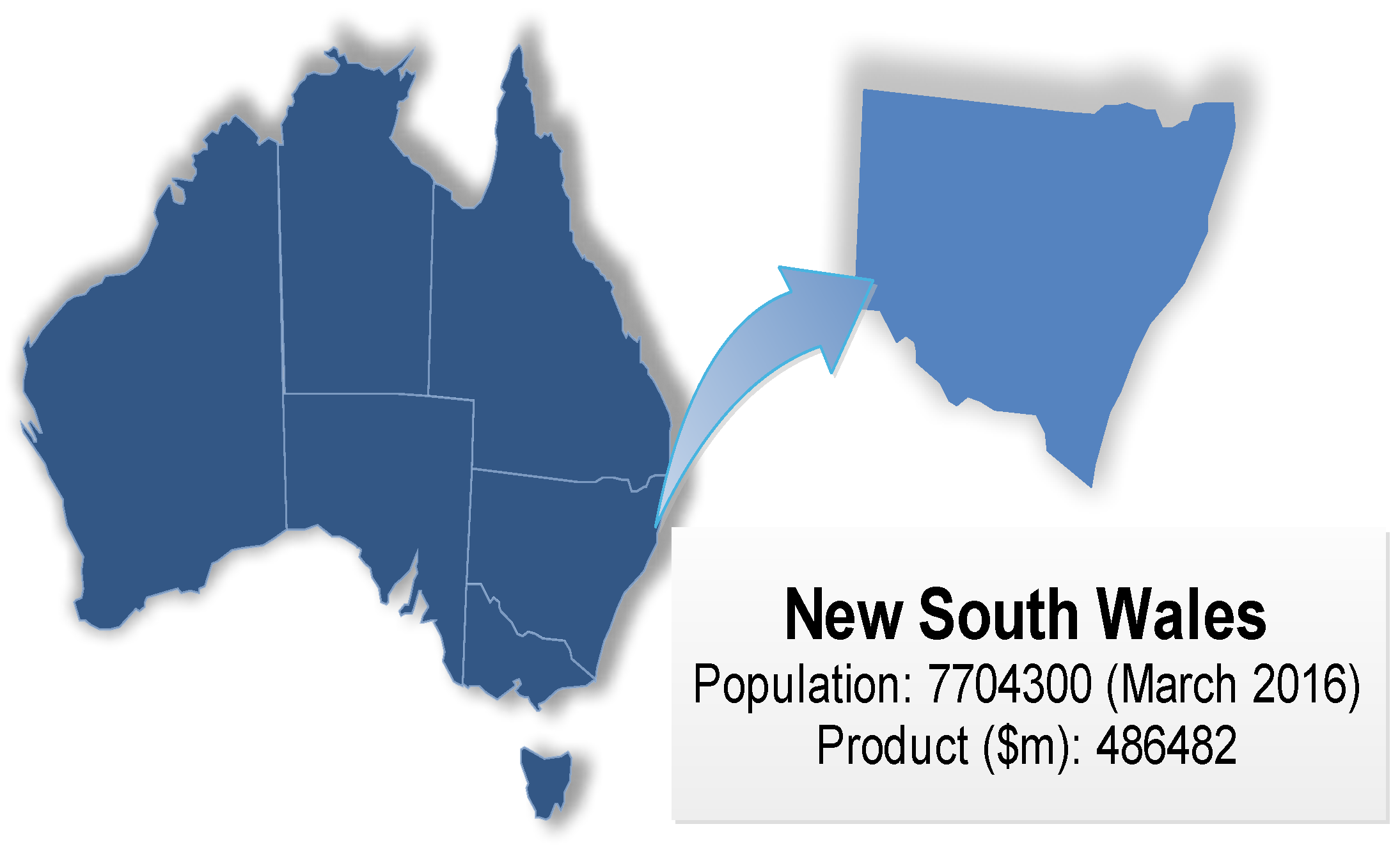
New South Wales is a state on the east coast of Australia (Figure 3). The estimated population of NSW at the end of March 2016 was 7.7 million, making it Australia’s most populous state. NSW is Australia’s economic powerhouse, and also one of the most active economic regions in the Asian-Pacific region. Among its industrial sectors, the most outstanding are the iron and steel industries. According to the data of the Australian immigration information network, the state’s GDP accounted for one third of Australia’s gross domestic product and more than 35% of the country’s products and services are manufactured in NSW. Its steel production accounted for about 85% of Australia’s total output, centering on the port of Newcastle and Ken Blah. Coal and related products are the state’s biggest exports. With an A$5 billion value, they account for about 19% of all exports. Electricity is inseparable from both industry and people’s life, and the electricity department must therefore ensure adequate power production.
3.2. Data Description
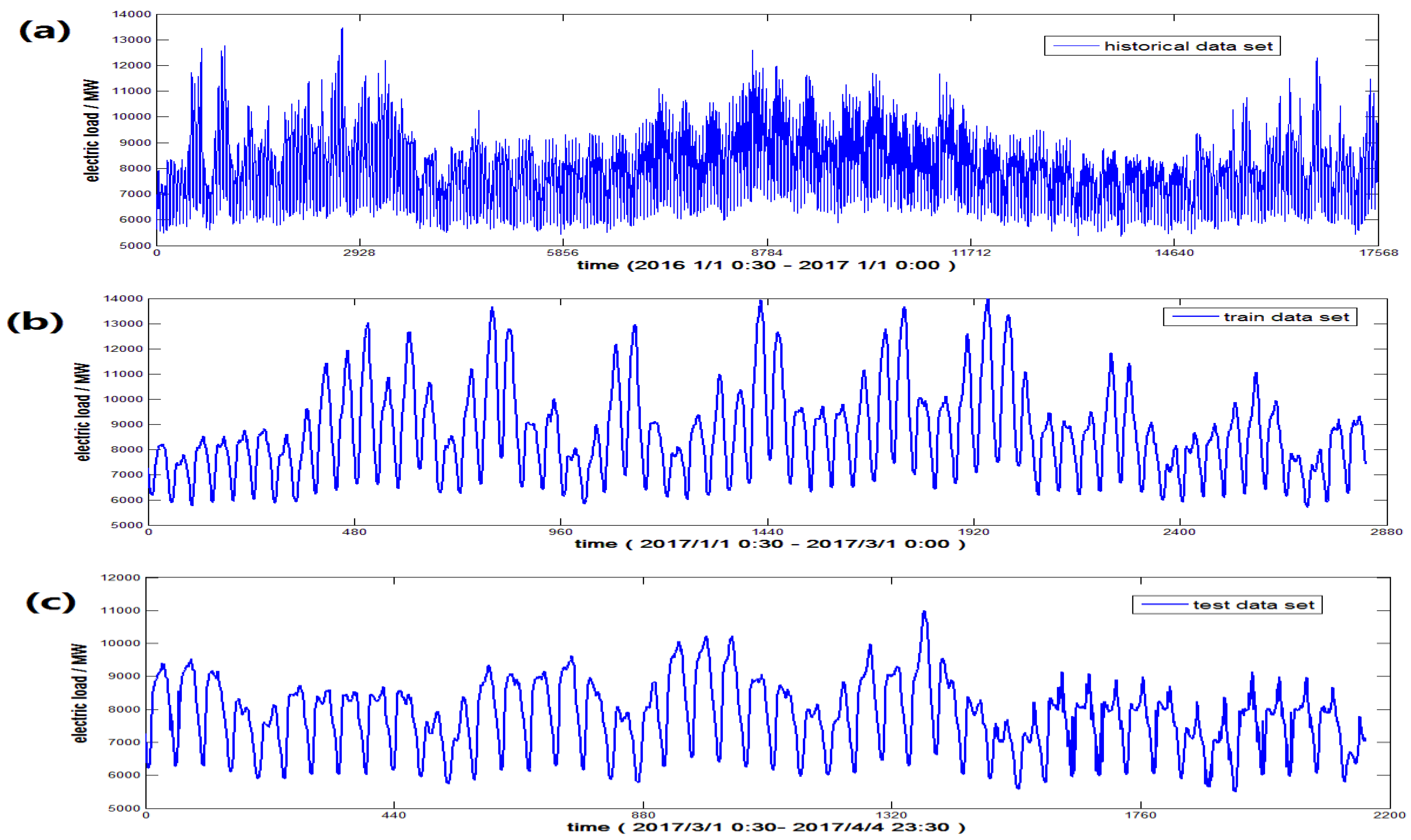
To verify the effectiveness of the proposed model, the data sets of electric load (Mw) from NSW (Australia) are used as the experimental data. They were obtained from the Australian Energy Market Operator (http://www.aemo.com.au/) [36]. Since the proposed hybrid model EWKM contains KNN and ELM, the sample data are divided into three groups: the first group is the historic subset of KNN, which contains 17,568 data points (from 1 January 2016 00:30 to 1 January 2017 00:00); the second is the training subset of ELM, which contains 2832 data points (from 1 January 2017 00:30 to 1 March 2017 00:00); the remaining 2158 data points (from 1 March 2017 00:30 to 14 April 2017 23:30) as the testing subset of ELM can be seen in Table 1 and Figure 4.
3.3. ELM-KNN as a Simulation Tool
The purpose of this section is to examine the fitting capacity of the combination of ELM and KNN for solving complex simulation problems. One thing that must be mentioned is that complex linear systems always appear in the application of projects, which can make it difficult to establish a suitable model, so there is a need for more research on how to find the reasonable and efficient methods to establish the nonlinear relationship between the input and the output. This section proposes a hybrid method that combines ELM and KNN. Three functions with different characteristics are employed as the benchmarks to prove its high fitting capacity. The structure of the three benchmarks considered in the experiment are as follows:
- F1: Sphere function (d = 2):
- F2: Rosenbrock function (d = 2):
- F3: Ackley function (d = 2):
The range of variables x1 and x2 are all from −2 to 2, with the step size of 0.04. That means the variables x1 and x2 have 101 possible values, respectively, and the algorithm can produce 10,201 groups of experimental data. After random ordering of these experimental data, all data are divided into three groups: the first group is the historical subset of KNN, which contains 8201 data points (from No. 1 to No. 8201); the second group is the training subset of ELM, which contains 1500 data points (from No. 8202 to No. 9701); the remaining 500 data points (from No. 9702 to No. 10,201) as the testing subset of ELM.
In order to prove the high fitting capacity of the proposed method ELM-KNN, three other method: KNN, BPNN-KNN and SVM-KNN are employed for comparison. After implementing these algorithms using Matlab 2014(b), we have carried out extensive simulations and each algorithm has been run 100 times so as to perform an average statistical analysis. Table 2 shows the results with the average value of sum error and time are taken as the criteria.
Multiple studies show that ELM-KNN can outperform KNN and other hybrid algorithm for solving non-linear simulation problems. The traditional KNN algorithm is suitable for solving linear problems, so although the run time is short, the sum error of this single algorithm is large. Therefore, this section take other algorithms which are suitable for non-linear fitting to combine with KNN. These hybrid algorithms are ELM-KNN, BPNN-KNN and SVM-KNN. It can be observed from Table 2 that while the accuracy of these hybrid algorithm is similar, the accuracy of ELM-KNN is slightly better than that of BPNN-KNN and SVM-KNN. More importantly, a marked improvement can be seen in the run speed with ELM-KNN. Each function evaluation is virtually instantaneous on a modern PC. For example, the computation time with ELM-KNN on a 2.13 GHz desktop is between 4 and 5 s, which was much superior to BPNN-KNN and SVM-KNN. These results show the high accuracy and efficiency of ELM-KNN that make it a very powerful tool for fitting.
3.4. Evaluation Criteria
The mean absolute error (MAE), the mean relative error (MRE) and the correlation coefficient (R) are used to evaluate the reliability of EWKM model. MAE and MRE measure residual errors, which give a global idea of the difference between the observed and forecasted values. MAE is used to evaluate the absolute error range of the predicted value, while MRE is used to reflect the specification of the predicted value on average. The lower the values of MAE and RMSE, the better the model is. The proportion of the total variance in the observed data can be described by the correlation coefficient (R). R is better when it is close to one.
MAE, MRE and R are calculated as follows:
where is the observed value, is the predictive value to , is the average of the observed value and n is the number of the observations of the validation set.
3.5. The Process of the Proposed Hybrid Model
3.5.1. Wavelet De-noising
The electrical demand is affected by a variety of factors, so electric load time series are usually accompanied by high noise. The direct forecasting of electric load with noisy data usually results in large errors. In this section, the DWT is executed for efficiently removing the noise from the observed data. In general, a normative procedure to select the decomposition level does not exist, so the selection is based on multiple experiments. In this study, the Daubechies wavelet of order 3 (db3) has a better performance, so the db3 is adopted in the wavelet denoising process [29,37]. Considering the characteristics of the experimental data, after testing the effect of different levels with db3, level 1 works best. The decomposition figure includes the approximation coefficients at level 1 (a1) and the detail coefficients at level 1 (d1). The decomposition process of the experimental data is shown in Figure 5. The a1 is a smoothed version of the original series and it represents the low frequency signal. Thus, a1 is selected to build forecasting model.
3.5.2. The Process of ELM-KNN
In Section 2.4, the EWKM hybrid model is established. The parameters of the hybrid model k = 12 are selected by lots of experiment tests. According to the choice of the electric load time series, there are 2832 training data from 1 January 2017 00:30 to 1 March 2017 00:00 (n = 2832) and 2158 testing data from 1 March 2017 00:30 to 14 April 2017 23:30 (m = 2158). Meanwhile, the half-hour electric load of the year 2016 (p = 17568) is selected as the historical data set in the experiment. Finally, the prediction of electric load could be calculated
3.6. Results and Analysis
3.6.1. Results of the Proposed Model
The results obtained from the modified hybrid model EWKM agree well with the original values. As is shown in Figure 6, the forecasting curve of EWKM closely approaches the original one. This figure confirms that the EWKM model has great performance in predicting the electric load series.
As Table 3 shows the MRE, R and MAE of the proposed model EWKM are 0.0262, 0.9660 and 196.7408, respectively.
The numerical value of the mean relative error (MRE) is close to zero and the correlation coefficient (R) is close to one. It clearly confirms that the EWKM model can capture the non-stationary and highly noisy features of the electric load series, and the new model can effectively improve the forecasting accuracy.
3.6.2. Model Comparisons
This section provides a comparison between the proposed EWKM model and three other benchmark models: EKM, WKM, and WNNM. Note that random selection of the parameters (ELM and BPNN) may cause different results. To prevent this uncertain phenomenon, fifty runs for each method are applied and the results of every run are recorded in Table 4.
The estimation performance of EWKM, EKM and WNNM are assessed by statistical indicators of MRE, MAE and R. The values are presented in Table 5. What needs special explanation is the fact that WKM is a non-parameter method and the result of this model is a fixed value, so it makes no sense to do lots of experiments with WKM. The mark “/” in Table 5 stands for the non-existent statistical values. To verify the EWKM model, this experiment compares it with EKM, WKM and WNNM, using the same electric load data. It must be noticed this analysis is done according to the mean value of three indicators. As listed in Table 5, EWKM has the lowest MRE, MAE and the highest R among the four models. Comparing EKM with EWKM, after introducing wavelet denoising into the model, the MRE and MAE have obviously decreased. Unlike the EKM model which is directly constructed from the original data, we decompose the original data into a low frequency and high frequencies parts, and the results indicate that the EWKM can capture the highly noisy and non-stationary features of electric load data after the wavelet denoising, so it can be concluded that the denoising process is crucial to predict electric loads. Then, comparing WKM with EWKM, the three average indicators MRE, R, MAE of the WKM are 0.0290, 0.9607 and 219.6566, respectively, which are all inferior to those of EWKM. This indicates that optimizing the kernel function by using the ELM has a wonderful effect, so the ELM is necessary to predict the electric load series. As for the WNNM, the BPNN is an artificial neural network which is widely used to predict time series. When using the BPNN to forecast electric loads, the two statistical errors MAE and MRE are clearly larger than the errors of the EWKM model. The comparison of the results between the four models shows that the proposed model EWKM can effectively improve forecasting accuracy. Therefore, the conclusion can be drawn that every part of the proposed model is suitable and reasonable. The proposed model EWKM that includes denoising processing, KNN and ELM constitutes a significant improvement in electric load forecasting.
4. Conclusions and Future Work
In electricity demand forecasting, noise signals, caused by various unstable factors, often corrupt electric load series. The contribution of this paper is a method that uses a hybrid model based on wavelet denoising processing. In previous studies, models had been usually established with the original data, however, this paper takes the low-frequency signal to modeling, so that it can reduce errors caused by noise signals. Moreover, in the construction of the kernel function, the traditional way is to construct a linear relationship, but this paper introduces the ELM into the establishment of the kernel function, so that it can optimize the KNN algorithm. Through the analysis of experimental results, a conclusion can be drawn that the every part included in the new hybrid model is necessary to predict future electric loads.
However, this paper only takes electric load data as the research subject, without taking other related variables into consideration. To resolve such limitations, future research should aim to include other factors which may influence the electric demand, such as the population and GDP, and there’s a lot of room for improvement.
Acknowledgments
The authors are grateful the editor and anonymous reviewers for their suggestions in proving the quality of the paper. This research is supported by the National Natural Sciences Foundation of China (No. 41571016).
Author Contributions
Weide Li designed research; Demeng Kong wrote the paper; Jinran Wu performed research and analyzed data.
Conflicts of Interest
The authors declare no conflict of interest.
Abbreviations
| ANN | artificial neural network |
| BAMO | binary animal migration optimization |
| BPNN | back propagation neural network |
| CS | cuckoo search algorithms |
| DWT | discrete wavelet transform |
| EEMD | ensemble empirical mode decomposition |
| EEuNN framework | evolving fuzzy neural network framework |
| ELM | extreme learning machine |
| EMD | empirical mode decomposition |
| FTS | fuzzy time series |
| GHSA | global harmony search algorithm |
| GM | grey model |
| GPRM | grey prediction with rolling mechanism |
| KNN regression | k-nearest neighbor regression |
| LSSVM | least squares support vector machines |
| MAE | mean absolute error |
| MRE | mean relative error |
| PSO | particle swarm optimization |
| QPSO | quantum particle swarm optimization algorithm |
| R | correlation coefficient |
| SARIMA | seasonal auto-regressive integrated moving average |
| SLFN | single hidden-layer feed-forward network |
| SSA | singular spectrum analysis |
| SVM | supporter vector machine |
| SVR | support vector regression |
| WT | wavelet transform |
References
- Goia, A.; May, C.; Fusai, G. Functional clustering and linear regression for peak load forecasting. Int. J. Forecast. 2010, 26, 700–711. [Google Scholar] [CrossRef]
- Zhou, P.; Ang, B.W.; Poh, K.L. A trigonometric grey prediction approach to forecasting electricity demand. Energy 2006, 31, 2839–2847. [Google Scholar] [CrossRef]
- Akay, D.; Atak, M. Grey prediction with rolling mechanism for electricity demand forecasting of Turkey. Energy 2007, 32, 1670–1675. [Google Scholar] [CrossRef]
- Chang, P.C.; Fan, C.Y.; Lin, J.J. Monthly electricity demand forecasting based on a weighted evolving fuzzy neural network approach. Int. J. Electr. Power Energy Syst. 2011, 33, 17–27. [Google Scholar] [CrossRef]
- Kavaklioglu, K. Modeling and prediction of Turkey’s electricity consumption using Support Vector Regression. Appl. Energy 2011, 88, 368–375. [Google Scholar] [CrossRef]
- Wang, J.; Zhu, W.; Zhang, W.; Sun, D. A trend fixed on firstly and seasonal adjustment model combined with the ε-SVR for short-term forecasting of electricity demand. Energy Policy 2009, 37, 4901–4909. [Google Scholar] [CrossRef]
- Kucukali, S.; Baris, K. Turkey’s short-term gross annual electricity demand forecast by fuzzy logic approach. Energy Policy 2010, 38, 2438–2445. [Google Scholar] [CrossRef]
- Dash, P.K.; Liew, A.C.; Rahman, S.; Ramakrishna, G. Building a fuzzy expert system for electric load forecasting using a hybrid neural network. Expert Syst. Appl. 1995, 9, 407–421. [Google Scholar] [CrossRef]
- Taylor, J.W. Triple seasonal methods for short-term electricity demand forecasting. Eur. J. Oper. Res. 2010, 204, 139–152. [Google Scholar] [CrossRef]
- Moghram, I.; Rahman, S. Analysis and evaluation of five short-term load forecasting techniques. IEEE Trans. Power Syst. 1989, 4, 1484–1491. [Google Scholar] [CrossRef]
- Wu, H.; Niu, D.; Song, Z. Short-term electric load forecasting based on data mining. Int. J. Eng. Technol. 2017, 8, 250–253. [Google Scholar] [CrossRef]
- Chen, H.Y.; Hong, W.-C.; Shen, W.; Huang, N.N. Electric load forecasting based on a least squares support vector machine with fuzzy time series and global harmony search algorithm. Energies 2016, 9, 70. [Google Scholar] [CrossRef]
- Huang, M.L. Hybridization of chaotic quantum particle swarm optimization with SVR in electric demand forecasting. Energies 2016, 9, 426. [Google Scholar] [CrossRef]
- Zhang, X.; Wang, J.; Zhang, K. Short-term electric load forecasting based on singular spectrum analysis and support vector machine optimized by Cuckoo search algorithm. Electr. Power Syst. Res. 2017, 146, 270–285. [Google Scholar] [CrossRef]
- Karlsson, M.S. Nearest Neighbor Regression Estimators in Rainfall-Runoff Forecasting. Ph.D. Thesis, University Of Arizona, Tucson, AZ, USA, 1985. [Google Scholar]
- Poloczek, J.; Andre Treiber, N.; Kramer, O. KNN regression as geo-impuation method for spatio-temporal wind data. In Proceedings of the International Joint Conference SOCO’14-CISIS’14-ICEUTE’14, Bilbao, Spain, 25–27 June 2014; Volume 299. [Google Scholar] [CrossRef]
- Ban, T.; Zhang, R.; Pang, S.; Sarrafzadeh, A.; Inoue, D. Referential KNN regression for financial time series forecasting. In Proceedings of the International Conference on Neural Information Processing, Daegu, Korea, 3–7 November 2013; Volume 8226, pp. 601–608. [Google Scholar]
- Hu, J.; Liu, J.; Liu, Y.; Gao, C. Emd-KNN model for annual average rainfall forecasting. J. Hydrol. Eng. 2013, 18, 1450–1457. [Google Scholar] [CrossRef]
- Li, X.; Ma, S.; Wang, Y. BamoKNN: A novel computational method for predicting the apoptpsis protein locations. In Proceedings of the IEEE International Conference on Bioinformatic & Biomedicine, Shenzhen, China, 15–18 December 2016; pp. 743–746. [Google Scholar]
- Wang, Y.; Nan, Z.; Chen, H.; Wu, X. Correction of daily precipitation data of ITPCAS dataset over the Qinghai-Tibetan plateau with KNN model. In Proceedings of the IGARSS IEEE International Geoscience & Remote Sensing Symposium, Beijing, China, 10–15 July 2016; pp. 593–596. [Google Scholar]
- Huang, G.B.; Rong, S.; You, K. Extreme learning machine:a new learning scheme of feedforward neural networks. In Proceedings of the International Joint Conference on Neural Networks, Budapest, Hungary, 25–29 July 2004; Volume 2, pp. 985–990. [Google Scholar]
- Ma, Z.; Luo, G.; Huang, D. Short term traffic flow prediction based on on-line sequential extreme learning machine. In Proceedings of the Eighth International Conference on Advanced Computational Intelligence, Chiang Mai, Thailand, 14–16 February 2016; pp. 143–149. [Google Scholar]
- Masri, D.; Woon, W.L.; Aung, Z. Soil property prediction: An extreme learning machine approach. In Proceedings of the International Conference on Neural Information Processing: Neural Information Processing, Istanbul, Turkey, 9–12 November 2015; pp. 18–27. [Google Scholar]
- Liao, H.Y.; Wang, H.; Hu, Z.J.; Wang, K.; Li, Y.; Huang, D.S.; Ning, W.H.; Zhang, C.X. Stock price forecasting based on extreme learning machine. Comput. Mod. 2014, 12. (In Chinese) [Google Scholar]
- Zhang, Y.H.; Wang, H.; Hu, Z.J.; Wang, K.; Li, Y. A hybrid short-term wind speed forecasting model based on wavelet decomposition and extreme learning machine. Adv. Mater. Res. 2013, 860–863, 361–367. [Google Scholar]
- Shamshirband, S.; Mohammadi, K.; Yee, D.L.; Petković, D.; Mostafaeipour, A. A comparative evaluation for identifying the suitability of extreme learning machine to predict horizontal global solar radiation. Renew. Sustain. Energy Rev. 2015, 52, 1031–1042. [Google Scholar] [CrossRef]
- Dabuechies, I. The wavelet transform, time-frequency loaclization and signal analysis. IEEE Trans. Inf. Theory 1990, 36, 6–7. [Google Scholar]
- Wang, L.P.; Shekhar, G. Neural networks and wavelet denoising for stock trading and prediction. Time Ser. Anal. Model. Appl. 2013, 47, 229–247. [Google Scholar]
- Wang, J.; Wang, J.; Li, Y.; Zhu, S.; Zhao, J. Techniques of applying wavelet denoising into a combined model for short-term load forecasting. Int. J. Electr. Power Energy Syst. 2014, 62, 816–824. [Google Scholar] [CrossRef]
- Qin, Y.; Huang, S.; Zhao, Q. Prediction model of chaotic time series based on wavelet denoising and LS-SVM and ITS application. J. Geod. Geodyn. 2008, 28, 96–100. [Google Scholar]
- Abbaszadeh, P. Improving hydrological process modeling using optimized threshold-based wavelet denoising technique. Water Resour. Manag. 2016, 30, 1701–1721. [Google Scholar] [CrossRef]
- Kalteh, A.M. Improving forecasting accuracy of streamflow time series using least squares support vector machine coupled with data-preprocessing techniques. Water Resour. Manag. 2016, 30, 747–766. [Google Scholar] [CrossRef]
- Liang, N.Y.; Huang, G.B.; Saratchandran, P.; Sundararajan, N. A fast and accurate on-line sequential learning algorithm for feedforward networks. IEEE Trans. Neural Netw. 2006, 17, 1411–1423. [Google Scholar] [CrossRef] [PubMed]
- Cover, T.M.; Hart, P.E. Nearest neighbor pattern classification. IEEE Trans. Inf. Theory 1967, 13, 21–27. [Google Scholar] [CrossRef]
- Lall, U.; Sharma, A. A nearest neighbor bootstrap for resampling hydrologic time series. Water Resour. Res. 1996, 32, 679–694. [Google Scholar] [CrossRef]
- Australian Energy Market Operator (AEMO). Available online: http://www.aemo.com.au (accessed on 12 May 2017).
- Ali, Y.M.K. Forecasting Power and Wind Speed Using Artificial and Wavelet Neural Networks for Prince Edward Island (PEI); Electrical and Computer Engineering at Dalhouse University: Halifax, NS, Canada, 2010. [Google Scholar]
Figure 1.
The structure of ELM.
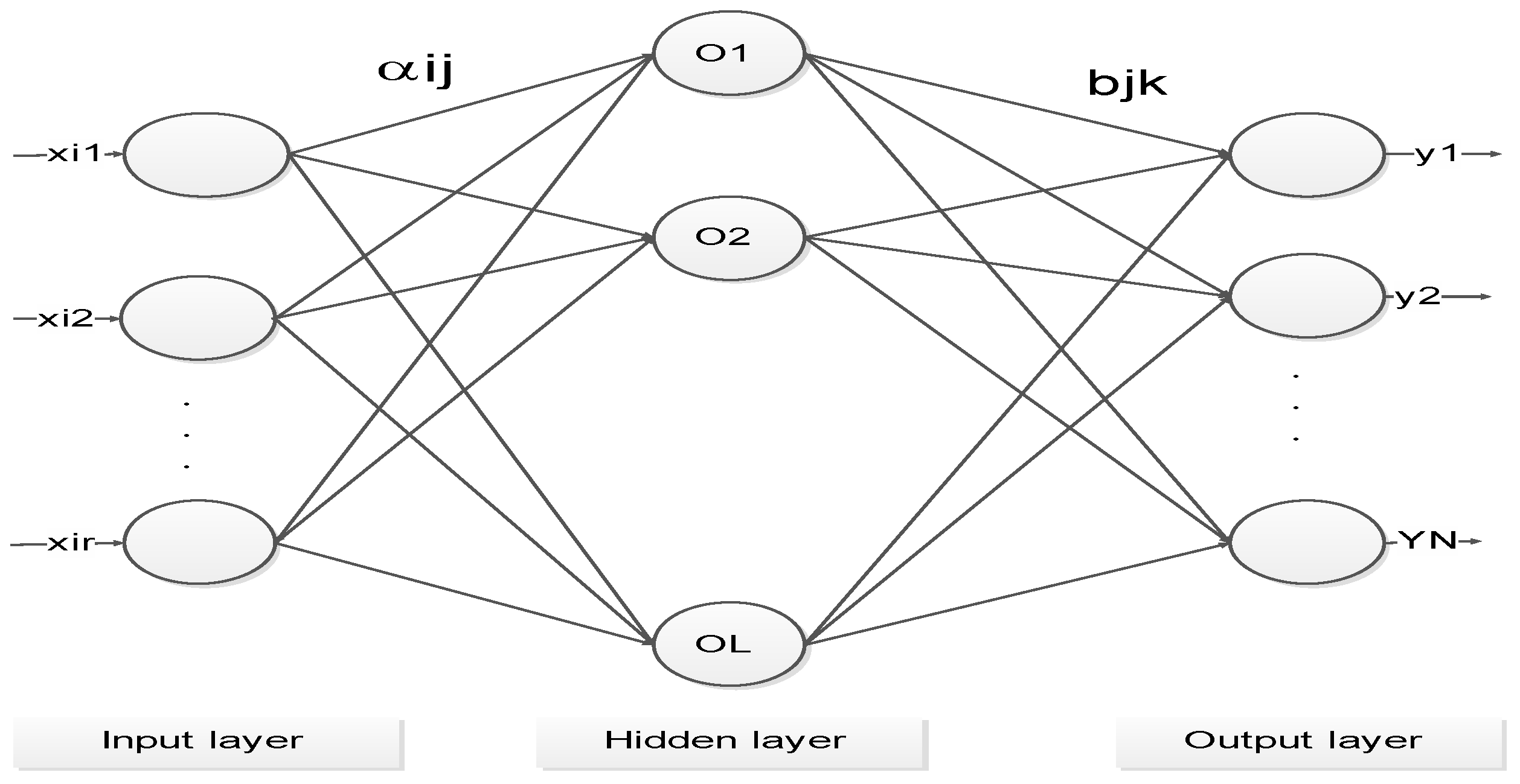
Figure 2.
The basic structure of the proposed model.
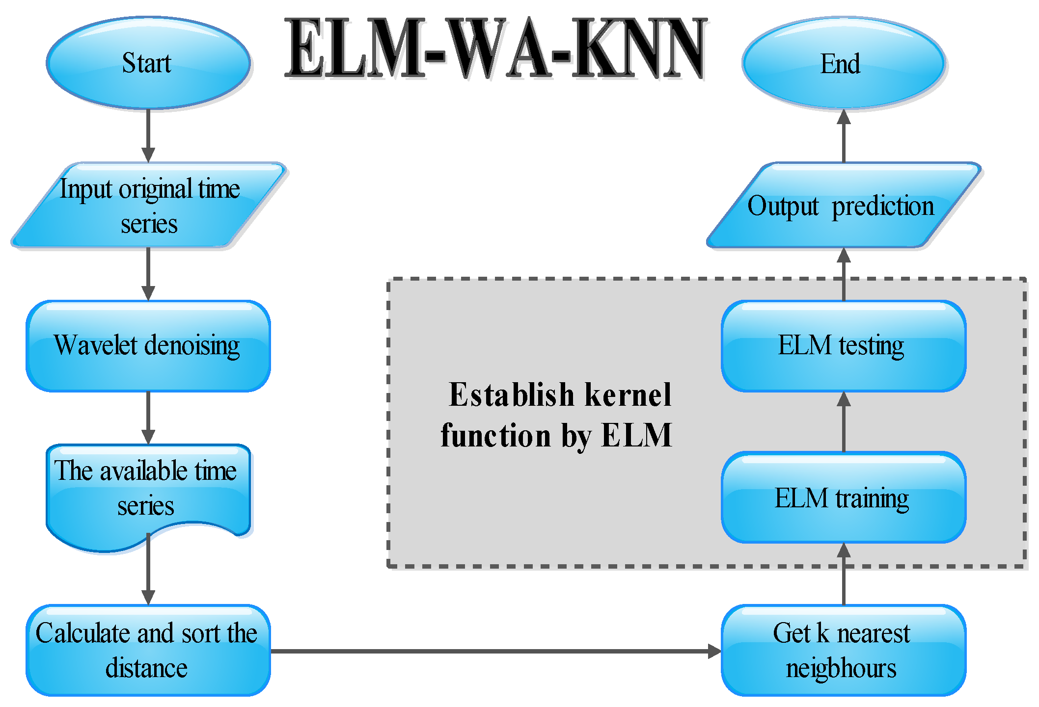
Figure 3.
The study area location.

Figure 4.
The electric load series of New Souths Wales, (a) historical data set; (b) train data set; (c) test data set.
Figure 4.
The electric load series of New Souths Wales, (a) historical data set; (b) train data set; (c) test data set.

Figure 5.
The process of wavelet denoising, (a) the decomposition of historical data set; (b) the decomposition of train and test data sets; note: a1, approximation signal; d1, detail signal.
Figure 5.
The process of wavelet denoising, (a) the decomposition of historical data set; (b) the decomposition of train and test data sets; note: a1, approximation signal; d1, detail signal.
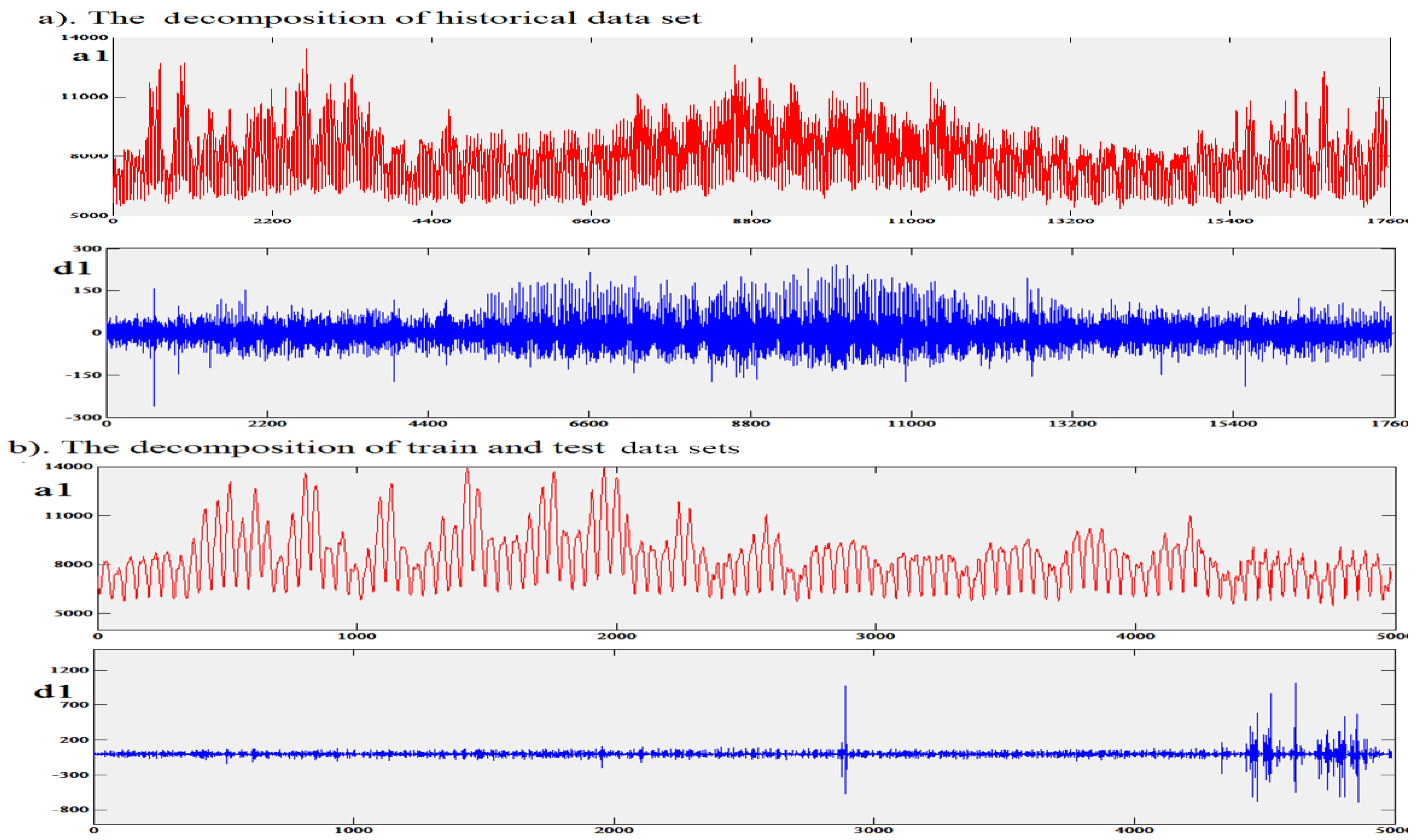
Figure 6.
Plot of the original data and predictive values.


Table 1.
Statistical parameters in each data set.
| Data Set | N | Min | Max | Mean | Std | S | K | ||
|---|---|---|---|---|---|---|---|---|---|
| Statistics | Std | Statistics | Std | ||||||
| Historical data set | 17,568 | 17,568 | 5350 | 13,459 | 7978 | 1257 | 0.473 | 0.018 | 0.185 |
| Train data of ELM | 2832 | 2832 | 5704 | 13,986 | 8612 | 1748 | 0.785 | 0.046 | 0.234 |
| Test data of ELM | 2158 | 2158 | 5489 | 11,000 | 7768 | 1044 | 0.000 | 0.053 | −0.557 |
Min is the minimum; Max is the maximum; Std is the standard deviation; S is the skewness; K is the kurtosis.
Table 2.
The Fitting performance of the four methods.
| Function | Criteria | KNN | ELM-KNN | BPNN-KNN | SVM-KNN |
|---|---|---|---|---|---|
| F1 | sum_error | 26.646 | 17.941 | 18.329 | 17.806 |
| time | 1.1875 | 4.7837 | 8.0738 | 6.8382 | |
| F2 | sum_error | 429.717 | 378.105 | 380.040 | 378.502 |
| time | 1.2615 | 4.6738 | 8.1256 | 6.9026 | |
| F3 | sum_error | 19.511 | 4.685 | 4.936 | 4.824 |
| time | 1.1701 | 4.8150 | 8.1373 | 6.8376 |
Table 3.
Indicators of the EWKM.
| Model | MRE | R | MAE |
|---|---|---|---|
| EWKM | 0.0262 | 0.9660 | 196.7408 |
Table 4.
The performance of the EWKM model compared to EKM and WNNM.
| Run No. | EWKM | EKM | WNNM | ||||||
|---|---|---|---|---|---|---|---|---|---|
| MRE | MAE | R | MRE | MAE | R | MRE | MAE | R | |
| 1 | 0.0272 | 203.9354 | 0.9643 | 0.0310 | 234.7119 | 0.9559 | 0.0340 | 258.2224 | 0.9484 |
| 2 | 0.0254 | 191.5216 | 0.9677 | 0.0330 | 247.7988 | 0.9513 | 0.0361 | 271.3461 | 0.9431 |
| 3 | 0.0262 | 197.2202 | 0.9658 | 0.0306 | 232.1543 | 0.9561 | 0.0336 | 255.2362 | 0.9487 |
| 4 | 0.0256 | 193.3032 | 0.9668 | 0.0331 | 248.1338 | 0.9495 | 0.0361 | 271.0228 | 0.9412 |
| 5 | 0.0269 | 200.0946 | 0.9652 | 0.0298 | 226.2427 | 0.9578 | 0.0328 | 249.4973 | 0.9509 |
| 6 | 0.0255 | 190.6721 | 0.9670 | 0.0324 | 244.7448 | 0.9519 | 0.0354 | 268.0375 | 0.9439 |
| 7 | 0.0267 | 199.5574 | 0.9654 | 0.0308 | 234.3278 | 0.9568 | 0.0342 | 260.6011 | 0.9491 |
| 8 | 0.0278 | 209.6388 | 0.9622 | 0.0306 | 232.2462 | 0.9575 | 0.0337 | 255.6075 | 0.9505 |
| 9 | 0.0256 | 191.8692 | 0.9669 | 0.0305 | 231.0665 | 0.9563 | 0.0336 | 254.9035 | 0.9487 |
| 10 | 0.0258 | 193.7943 | 0.9662 | 0.0312 | 237.2551 | 0.9540 | 0.0344 | 261.8085 | 0.9459 |
| 11 | 0.0264 | 198.3134 | 0.9645 | 0.0328 | 245.2984 | 0.9522 | 0.0355 | 266.4726 | 0.9442 |
| 12 | 0.0265 | 197.8550 | 0.9654 | 0.0308 | 233.8156 | 0.9557 | 0.0338 | 256.7917 | 0.9483 |
| 13 | 0.0261 | 195.9784 | 0.9663 | 0.0311 | 236.2416 | 0.9545 | 0.0344 | 261.1275 | 0.9463 |
| 14 | 0.0265 | 198.5158 | 0.9656 | 0.0302 | 229.5213 | 0.9575 | 0.0334 | 253.4824 | 0.9501 |
| 15 | 0.0253 | 190.1162 | 0.9676 | 0.0336 | 255.4914 | 0.9500 | 0.0362 | 275.4577 | 0.9433 |
| 16 | 0.0254 | 190.7357 | 0.9674 | 0.0323 | 243.8135 | 0.9523 | 0.0349 | 263.8025 | 0.9451 |
| 17 | 0.0274 | 205.2306 | 0.9633 | 0.0309 | 232.5388 | 0.9557 | 0.0342 | 257.9839 | 0.9472 |
| 18 | 0.0271 | 200.2789 | 0.9657 | 0.0315 | 237.7104 | 0.9543 | 0.0346 | 261.7518 | 0.9460 |
| 19 | 0.0250 | 187.6062 | 0.9684 | 0.0330 | 246.9160 | 0.9512 | 0.0356 | 267.7434 | 0.9431 |
| 20 | 0.0257 | 192.4959 | 0.9671 | 0.0310 | 234.3247 | 0.9556 | 0.0342 | 258.7666 | 0.9475 |
| 21 | 0.0261 | 196.6063 | 0.9666 | 0.0334 | 251.6897 | 0.9493 | 0.0365 | 275.8747 | 0.9407 |
| 22 | 0.0256 | 193.2492 | 0.9668 | 0.0337 | 251.4458 | 0.9491 | 0.0367 | 274.8453 | 0.9409 |
| 23 | 0.0267 | 200.5948 | 0.9646 | 0.0315 | 237.0884 | 0.9553 | 0.0345 | 260.6253 | 0.9478 |
| 24 | 0.0258 | 195.8141 | 0.9664 | 0.0298 | 226.9438 | 0.9581 | 0.0329 | 250.6053 | 0.9508 |
| 25 | 0.0266 | 199.7260 | 0.9654 | 0.0302 | 230.2009 | 0.9572 | 0.0334 | 254.9789 | 0.9497 |
| 26 | 0.0253 | 191.2983 | 0.9676 | 0.0304 | 230.2200 | 0.9570 | 0.0336 | 255.1938 | 0.9493 |
| 27 | 0.0271 | 204.0736 | 0.9641 | 0.0306 | 232.7197 | 0.9564 | 0.0336 | 256.5639 | 0.9490 |
| 28 | 0.0265 | 199.2113 | 0.9654 | 0.0336 | 253.1185 | 0.9494 | 0.0365 | 276.1422 | 0.9412 |
| 29 | 0.0278 | 207.2988 | 0.9639 | 0.0308 | 232.1803 | 0.9559 | 0.0337 | 254.5038 | 0.9483 |
| 30 | 0.0265 | 196.9944 | 0.9666 | 0.0312 | 236.7581 | 0.9545 | 0.0344 | 261.5399 | 0.9468 |
| 31 | 0.0250 | 186.9544 | 0.9681 | 0.0319 | 241.2899 | 0.9524 | 0.0351 | 266.2253 | 0.9437 |
| 32 | 0.0280 | 208.4472 | 0.9630 | 0.0311 | 234.4506 | 0.9548 | 0.0343 | 258.7330 | 0.9469 |
| 33 | 0.0254 | 191.0999 | 0.9674 | 0.0330 | 249.9862 | 0.9509 | 0.0361 | 273.8056 | 0.9431 |
| 34 | 0.0255 | 191.7066 | 0.9670 | 0.0303 | 229.5405 | 0.9570 | 0.0334 | 252.9284 | 0.9495 |
| 35 | 0.0259 | 194.0202 | 0.9665 | 0.0305 | 231.5181 | 0.9565 | 0.0332 | 252.7351 | 0.9498 |
| 36 | 0.0262 | 196.7985 | 0.9661 | 0.0341 | 256.5269 | 0.9490 | 0.0370 | 279.2929 | 0.9411 |
| 37 | 0.0258 | 193.2783 | 0.9663 | 0.0317 | 241.1737 | 0.9530 | 0.0348 | 265.5501 | 0.9448 |
| 38 | 0.0265 | 199.2508 | 0.9646 | 0.0324 | 244.2265 | 0.9515 | 0.0352 | 266.1942 | 0.9442 |
| 39 | 0.0270 | 201.3869 | 0.9651 | 0.0306 | 232.2034 | 0.9563 | 0.0336 | 255.2785 | 0.9493 |
| 40 | 0.0265 | 200.2736 | 0.9652 | 0.0321 | 243.9047 | 0.9526 | 0.0352 | 267.3854 | 0.9448 |
| 41 | 0.0278 | 207.9120 | 0.9631 | 0.0321 | 241.4578 | 0.9526 | 0.0350 | 264.2843 | 0.9442 |
| 42 | 0.0251 | 188.3151 | 0.9683 | 0.0321 | 242.7873 | 0.9536 | 0.0349 | 264.5100 | 0.9462 |
| 43 | 0.0260 | 194.4705 | 0.9662 | 0.0313 | 238.4554 | 0.9546 | 0.0345 | 263.1648 | 0.9468 |
| 44 | 0.0257 | 192.4090 | 0.9678 | 0.0304 | 231.6317 | 0.9575 | 0.0336 | 256.3101 | 0.9503 |
| 45 | 0.0249 | 187.3678 | 0.9686 | 0.0312 | 237.9146 | 0.9538 | 0.0345 | 262.7347 | 0.9457 |
| 46 | 0.0273 | 205.1311 | 0.9638 | 0.0320 | 243.1807 | 0.9530 | 0.0352 | 267.2574 | 0.9451 |
| 47 | 0.0250 | 187.8190 | 0.9682 | 0.0306 | 231.5329 | 0.9568 | 0.0338 | 256.1022 | 0.9485 |
| 48 | 0.0290 | 214.2247 | 0.9622 | 0.0328 | 247.6485 | 0.9496 | 0.0359 | 272.0024 | 0.9411 |
| 49 | 0.0252 | 189.6822 | 0.9674 | 0.0315 | 238.6218 | 0.9527 | 0.0345 | 261.9417 | 0.9450 |
| 50 | 0.0256 | 192.8932 | 0.9666 | 0.0313 | 237.3966 | 0.9547 | 0.0347 | 264.2695 | 0.9465 |
Table 5.
Comparing the three criteria of four models.
| Indicators | Models | Mean | Minimum | Maximum | Standard Deviation | Median | Upper Quantile | Lower Quantile |
|---|---|---|---|---|---|---|---|---|
| MRE | EWKM | 0.0262 | 0.0249 | 0.0290 | 0.0009 | 0.0261 | 0.0255 | 0.0267 |
| EKM | 0.0316 | 0.0298 | 0.0341 | 0.0011 | 0.0313 | 0.0306 | 0.0324 | |
| WNNM | 0.0346 | 0.0328 | 0.0370 | 0.0011 | 0.0345 | 0.0337 | 0.0352 | |
| WKM | 0.0290 | / | / | / | / | / | / | |
| MAE | EWKM | 196.7408 | 186.9544 | 214.2247 | 6.4440 | 196.2924 | 191.7473 | 200.2289 |
| EKM | 238.8433 | 226.2427 | 256.5269 | 7.7976 | 237.3259 | 232.2141 | 244.1461 | |
| WNNM | 262.4248 | 249.4973 | 279.2929 | 7.4146 | 261.7802 | 256.1542 | 267.0612 | |
| WKM | 219.6566 | / | / | / | / | / | / | |
| R | EWKM | 0.9660 | 0.9622 | 0.9686 | 0.0016 | 0.9663 | 0.9651 | 0.9671 |
| EKM | 0.9540 | 0.9490 | 0.9581 | 0.0027 | 0.9545 | 0.9522 | 0.9563 | |
| WNNM | 0.9463 | 0.9407 | 0.9509 | 0.0030 | 0.9464 | 0.9442 | 0.9487 | |
| WKM | 0.9607 | / | / | / | / | / | / |
© 2017 by the authors. Licensee MDPI, Basel, Switzerland. This article is an open access article distributed under the terms and conditions of the Creative Commons Attribution (CC BY) license (http://creativecommons.org/licenses/by/4.0/).
Share and Cite
MDPI and ACS Style
Li, W.; Kong, D.; Wu, J. A Novel Hybrid Model Based on Extreme Learning Machine, k-Nearest Neighbor Regression and Wavelet Denoising Applied to Short-Term Electric Load Forecasting. Energies 2017, 10, 694. https://doi.org/10.3390/en10050694
AMA Style
Li W, Kong D, Wu J. A Novel Hybrid Model Based on Extreme Learning Machine, k-Nearest Neighbor Regression and Wavelet Denoising Applied to Short-Term Electric Load Forecasting. Energies. 2017; 10(5):694. https://doi.org/10.3390/en10050694
Chicago/Turabian StyleLi, Weide, Demeng Kong, and Jinran Wu. 2017. "A Novel Hybrid Model Based on Extreme Learning Machine, k-Nearest Neighbor Regression and Wavelet Denoising Applied to Short-Term Electric Load Forecasting" Energies 10, no. 5: 694. https://doi.org/10.3390/en10050694
Note that from the first issue of 2016, this journal uses article numbers instead of page numbers. See further details here.