
An On-Board Remaining Useful Life Estimation Algorithm for Lithium-Ion Batteries of Electric Vehicles


Faculty of Transportation Engineering, Kunming University of Science and Technology, Kunming 650500, China
*
Author to whom correspondence should be addressed.
Energies 2017, 10(5), 691; https://doi.org/10.3390/en10050691
Submission received: 20 March 2017
/
Revised: 8 May 2017
/
Accepted: 11 May 2017
/
Published: 14 May 2017
(This article belongs to the Section D: Energy Storage and Application)
Abstract
:Battery remaining useful life (RUL) estimation is critical to battery management and performance optimization of electric vehicles (EVs). In this paper, we present an effective way to estimate RUL online by using the support vector machine (SVM) algorithm. By studying the characteristics of the battery degradation process, the rising of the terminal voltage and changing characteristics of the voltage derivative (DV) during the charging process are introduced as the training variables of the SVM algorithm to determine the battery RUL. The SVM is then applied to build the battery degradation model and predict the battery real cycle numbers. Experimental results prove that the built battery degradation model shows higher accuracy and less computation time compared with those of the neural network (NN) method, thereby making it a potential candidate for realizing online RUL estimation in a battery management system (BMS).
1. Introduction
Currently, lithium-ion batteries are widely employed as the main power source of electric vehicles (EVs). Compared with other prevalent solutions, lithium-ion batteries have the advantages of high energy density, high power density, low self-discharge rate, and no memory effect [1,2]. To meet operational power and energy demands, the lithium-ion battery packs in EVs are composed of hundreds to thousands of cells connected in series, parallel, or even more complex manners. Hence, it is imperative to guarantee and oversee the battery pack’s proper operation [3,4]. A commonly-accepted solution is that a battery management system (BMS) is employed to monitor a battery pack’s status and ensure its safety and performance optimization. For the BMS, a key function is to estimate the state of charge (SOC) and state of health (SOH) of the battery [5,6]. The SOC is usually defined as the ratio of the remaining capacity over the rated value, and the SOH describes the battery’s physical health condition compared with that of a fresh battery. Battery remaining useful life (RUL) is a different form of SOH, which is defined as the difference between the actual cycle number and the total cycle number. For EV applications, the total cycle number can be calculated when the battery capacity drops to eighty percent of the rated capacity, which is normally regarded as the end of life (EOL). It is quite difficult to estimate the battery actual cycle number during the charge/discharge process though; a variety of studies have tried to find connections between the charging voltage, current profiles, and cycle numbers, thereby determining its value.
Recent studies show that RUL is one of the main research interests in the field of battery status estimation, producing a pool of valuable publications. In general, RUL can be determined based on the increased internal resistance and the decreased capacity of the battery. In [7], a genetic algorithm (GA) is harnessed to estimate the internal resistance based on an equivalent circuit model (ECM). Then the relationship between the internal resistance and the degradation of the battery capacity is obtained. Similarly, the detailed relationship between the internal impedance and capacity, revealing the degradation condition of the battery, is presented in [4]. In [8], a number of experiments at different health conditions were carried out to obtain the corresponding battery capacity. An empirical exponential method is applied to fit the battery capacity with the aging condition of the battery. In [9], integration of the empirical exponential method with a polynomial regression equation is applied to improve the model fitting precision based on the findings of [8]. In [10,11], five characteristic values are extracted for building the lithium-ion battery capacity degradation model during the charging process. A clustering analysis algorithm, named KNN, and a sparse Bayesian learning method are respectively applied to establish the battery degradation model.
Normally, the RUL is closely related to the battery internal resistance and capacity, but the recent research findings in [12,13,14,15] show that the charging and discharging terminal voltages may also have an important effect on estimating the RUL. In [16], the charging terminal voltage with varied cycle curves under different health conditions is analyzed based on a feed-forward neural network (FNN). The aforementioned methods are primarily based on a single characteristic value under different cycle numbers; however, during the sampling process, this specific variable can easily suffer from measurement noise. Thus, the accuracy of the estimation will possibly be reduced. Therefore, a variety of studies on battery RUL estimation based on the relationship between battery capacity and voltage has been proposed in [17,18,19]. In [17], the incremental capacity analysis (ICA) method is applied to investigate the capacity difference in voltage plateau regions with different cycles. Then the incremental capacity is employed to estimate the RUL. In [20], the differential value between capacity and voltage is used to obtain the battery RUL. In [21], the researchers analyzed the voltage derivative (DV) curves during the charging process and fit the terminal DV curves under different cycle numbers. Then two inflection points at the initial and terminal stages are separately employed to estimate the charging capacity for a battery in different health conditions.
Based on the relationships between RUL and the internal resistance, the decreased capacity, the DV, and the terminal charging voltages, a variety of filter algorithms are proposed to improve the accuracy and robustness of the RUL estimation. In [22], the symbolic dynamic filtering algorithm (SDF) is employed to estimate battery RUL by processing the data based on the discrete wavelet transform (DWT). The battery parameters can be estimated by the SDF algorithm and, thus, the battery RUL is determined. In [23], a mixture of Gaussian algorithm processes adapts to learn the battery parameters under different health conditions and to produce a variety of particles. These particles are used as input variables for the particle filter (PF) algorithm to estimate the SOH and RUL. In [24], a dual extended Kalman filter (DEKF) is proposed to estimate the battery SOC and SOH. The battery SOC is estimated by one KF and the battery parameters, some of which can determine the battery SOH, are updated offline by the other KF.
In addition to filter algorithms, there exists an abundance of algorithms for RUL estimation based on statistical theory and pattern recognition, such as Bayesian theory [25,26,27], neural networks (NN) and various transformers [16,28], support vector machine (SVM) algorithms [19,25,29,30], etc. The NN and SVM algorithms both have remarkable advantages in dealing with nonlinear modeling problems. However, the NN obtains the optimal model by a local search method rather than global optimization. Compared with the NN, the SVM algorithm not only has a global optimal searching capability, but also bases itself on the non-linear classification theory, thus improving the search efficiency. In [31,32], the battery model is built based on a data-driven method. Then the SVM is applied to deal with the large amount of data by transforming high-dimensional data into low-dimensional data, finally proving that the SVM model can effectively predict the battery SOH and RUL. Compared with the algorithms mentioned above, the SVM operating process can have rapid convergence speed and stronger robustness. Considering these merits, the SVM algorithm is employed in this paper to predict battery RUL. In addition, more effective characteristics of the battery regression are extracted as training samples to build the SVM model. Firstly, according to the different battery charging times, the terminal voltages under different health conditions can be classified into four parts during the charging process. Secondly, when the battery voltage is close to the high cut-off voltage, the DV is also divided into four parts. The terminal voltage and DV values in the two steps listed above are employed as training data and result validation data, respectively, for the SVM model of battery regression. The SVM algorithm is then applied to predict the actual cycle numbers of the battery and to estimate the battery RUL. Finally, experimental results validate the feasibility of the proposed algorithm.
2. Battery Data Preparation
2.1. Battery Test
For lithium-ion batteries, the charging voltage and current responses change with the increment of the charge/discharge cycles. In this paper, all of the experimental data are acquired from an Arbin tester, BT-2000 (College Station, TX, USA), associated with a thermal chamber, PunDun-GDW100L. The Arbin tester implements battery charge and discharge operations and the chamber ensures the battery temperature remains unchanged during the charging and discharging process.
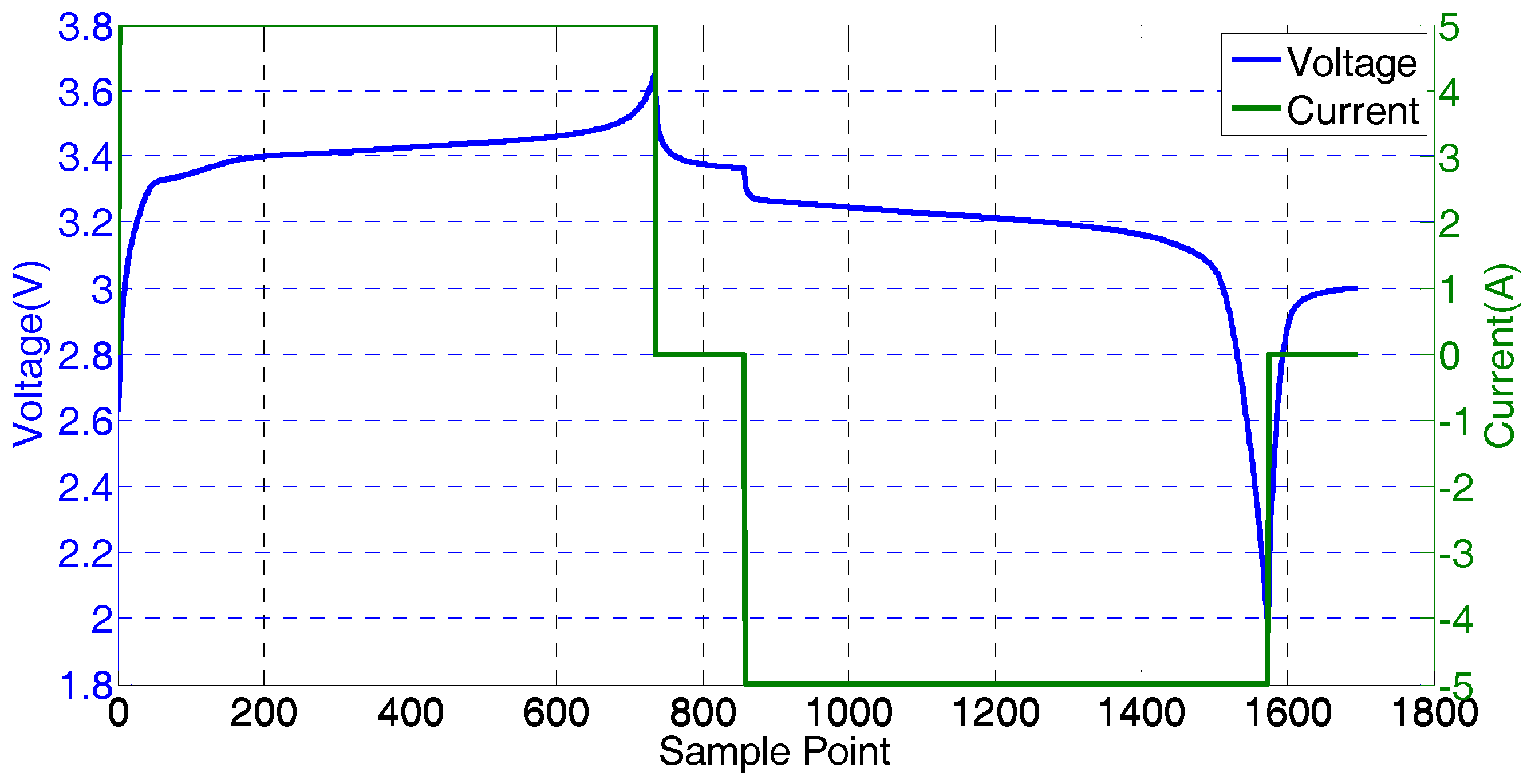
In this paper, the experimental battery capacity is that of a lithium-ion phosphate cell with a rated capacity of 5 Ah and rated voltage of 3.3 V. As shown in Figure 1, the blue line represents the battery voltage response curve and the green line indicates the charging current, which is constant at 1, where denotes the normal capacity of the battery with the unit Ah. The rated capacity of the battery is 5 Ah, thus equals 5. When the terminal voltage reaches the high cut-off voltage of 3.65 V, the charging process will stop, followed by rest for a certain duration of time. Meanwhile, during the discharging process the current will be stopped when the terminal voltage arrives at the low cut-off voltage of 2.0 V. The whole process is measured under a fixed temperature, i.e., 25 °C. Due to the abundant test data, the sampling frequency is set to be 5 s. Generally, the battery charge process contains two stages: the constant current (CC) process and the constant voltage (CV) process. In the CC stage, the charging terminal voltage features obvious differences when degradation occurs, and the primary aim of the experiment is to extract the characteristic values based on the terminal voltage. In the CV stage, the charging capacity changes within relatively limited boundaries, the terminal voltage remains unchanged, and the current decreases gradually. If we consider the signal variation during the CV process, the only way is the current values. Thus, it increases the number of variables, thereby increasing the computational complexity. To sum up, we only considered the voltage variation during the CC stage to extract features for modeling the battery degradation. To shorten the test time without obviously influencing the precision, we set the rest time as 10 minutes. It is necessary to mention that in order to easily compare the degradation and extract the characteristic value for the modeling process, we employ the sample point as the horizontal coordinate instead of time.
2.2. Analysis of the Characteristics of Battery Degradation
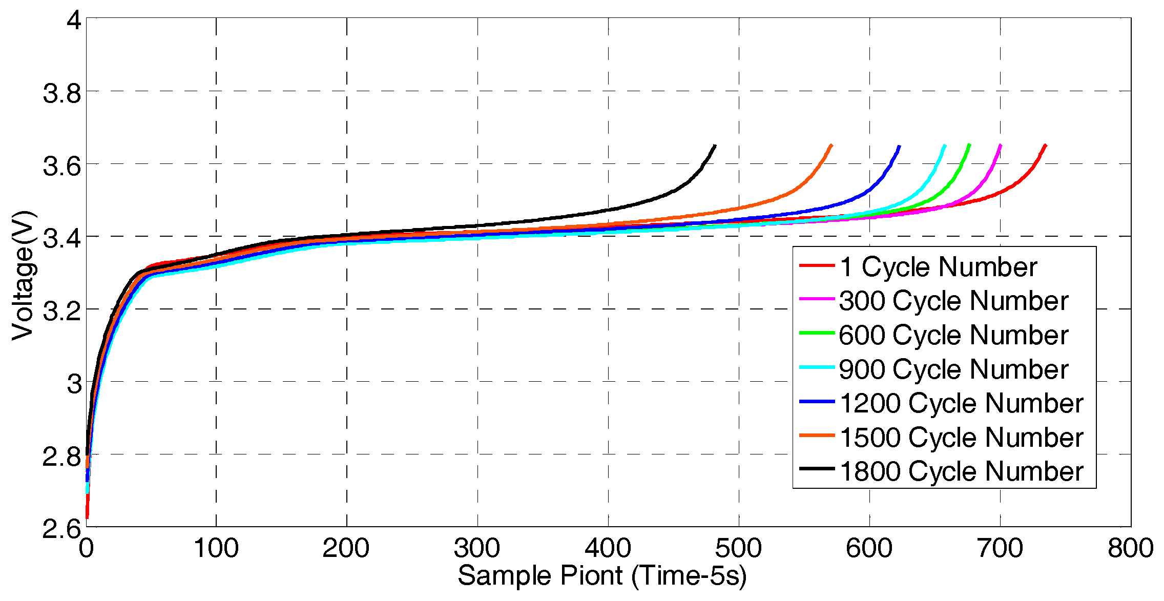
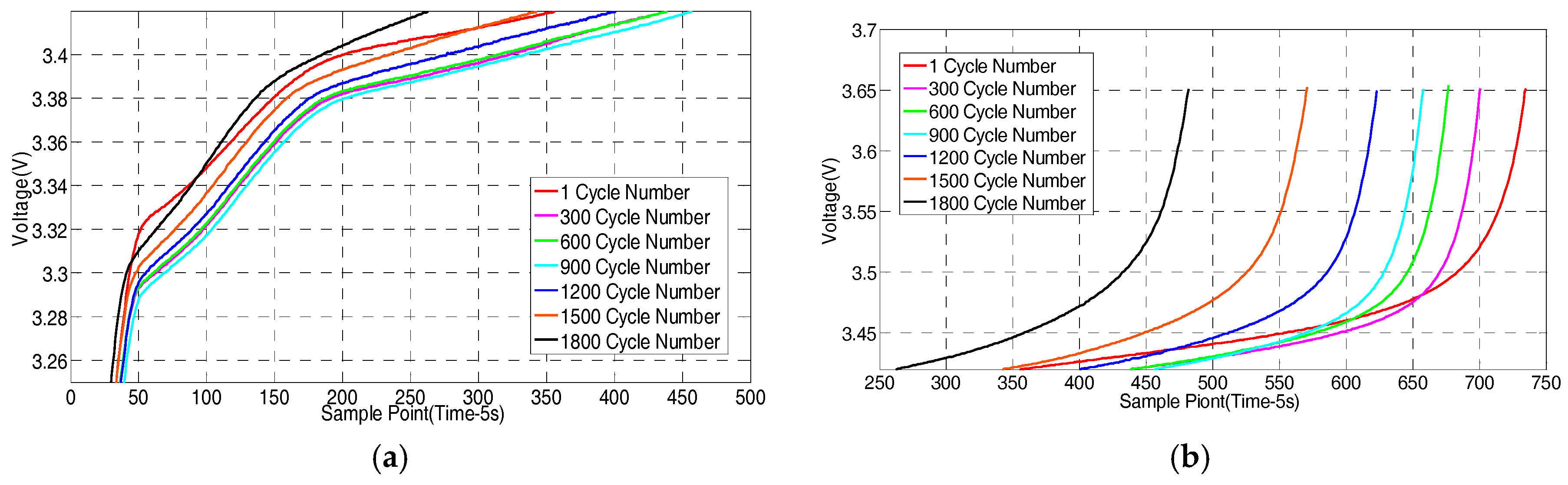
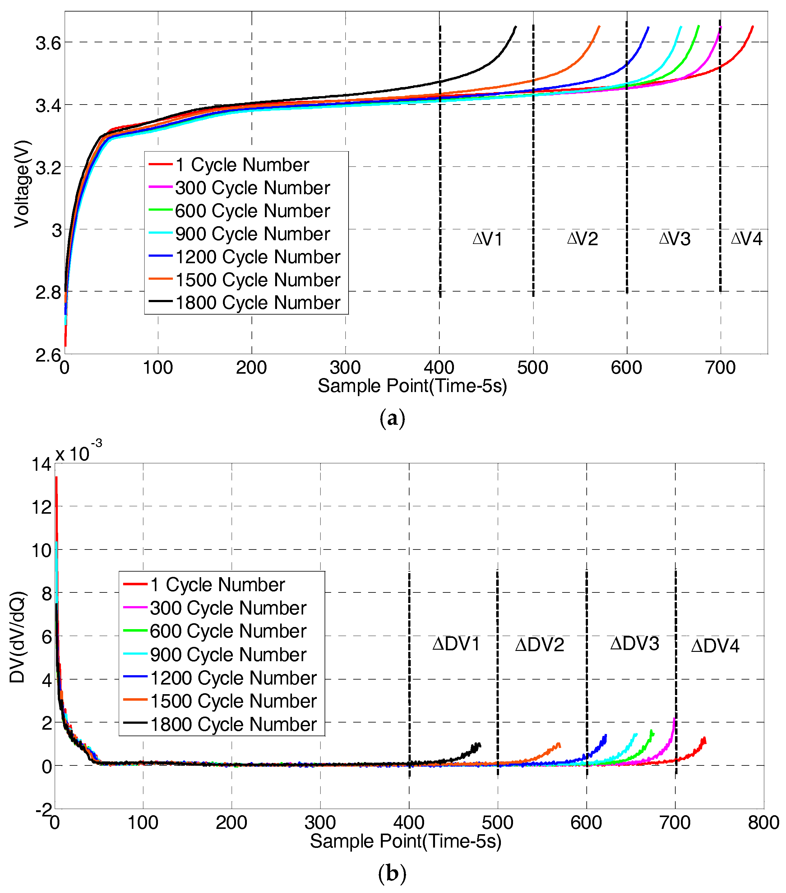
After a number of charging/discharging cycles, the cathode/anode’s materials and the electrolytes in the battery gradually change due to complex physical and chemical reactions which, in turn, brings an increment of the internal resistance and a decrement of the available capacity. In EVs, when the actual battery capacity drops to 80% of its normal value, a common fact is that the output power of the battery cannot meet the EV’s requirement and, thus, the battery must be replaced. During the charge experiment, eight batteries are chosen to test for acquiring the charge voltage and current responses, and only one battery test datum is applied to study the battery degradation condition at the end. The battery data is divided into seven groups with intervals of 300 cycles, as shown in Figure 2. It is worth noting that all of the voltages change slightly in the voltage plateau region; however, the aged batteries have less charging time compared with that of the fresh ones. Thus, according to the terminal voltage of each charging process, the battery health states can be predicted. That said, since the battery internal impedance does not noticeably change, this method cannot estimate the battery health condition accurately. The charging capacity under different cycle numbers is shown in Figure 3. All batteries under different health conditions have the same charging cut-off voltage. Obviously, the capacity of a fresh battery is more than its rated capacity. The battery capacity is reduced by approximately 6% when the cycle number equals 600. The battery capacity reaches close to EOL when the battery is operated for 1500 cycles. During cycle numbers 1 through 1500, the battery capacity decreases slowly. The battery capacity decreases rapidly when the cycle number exceeds 1500 and the ultimate capacity is only 65% when the battery cycle is 1800. As shown in Figure 4, the charging process can be divided into two sub-processes: (1) a voltage plateau region during the sampling portion from sample points 30–400; and (2) the terminal voltage region during the sampling portion from sample points 400 to the end. The voltage changes dramatically with the increase of cycle numbers in the terminal voltage region, while remaining almost unchanged as the cycle number increases in the voltage plateau region.
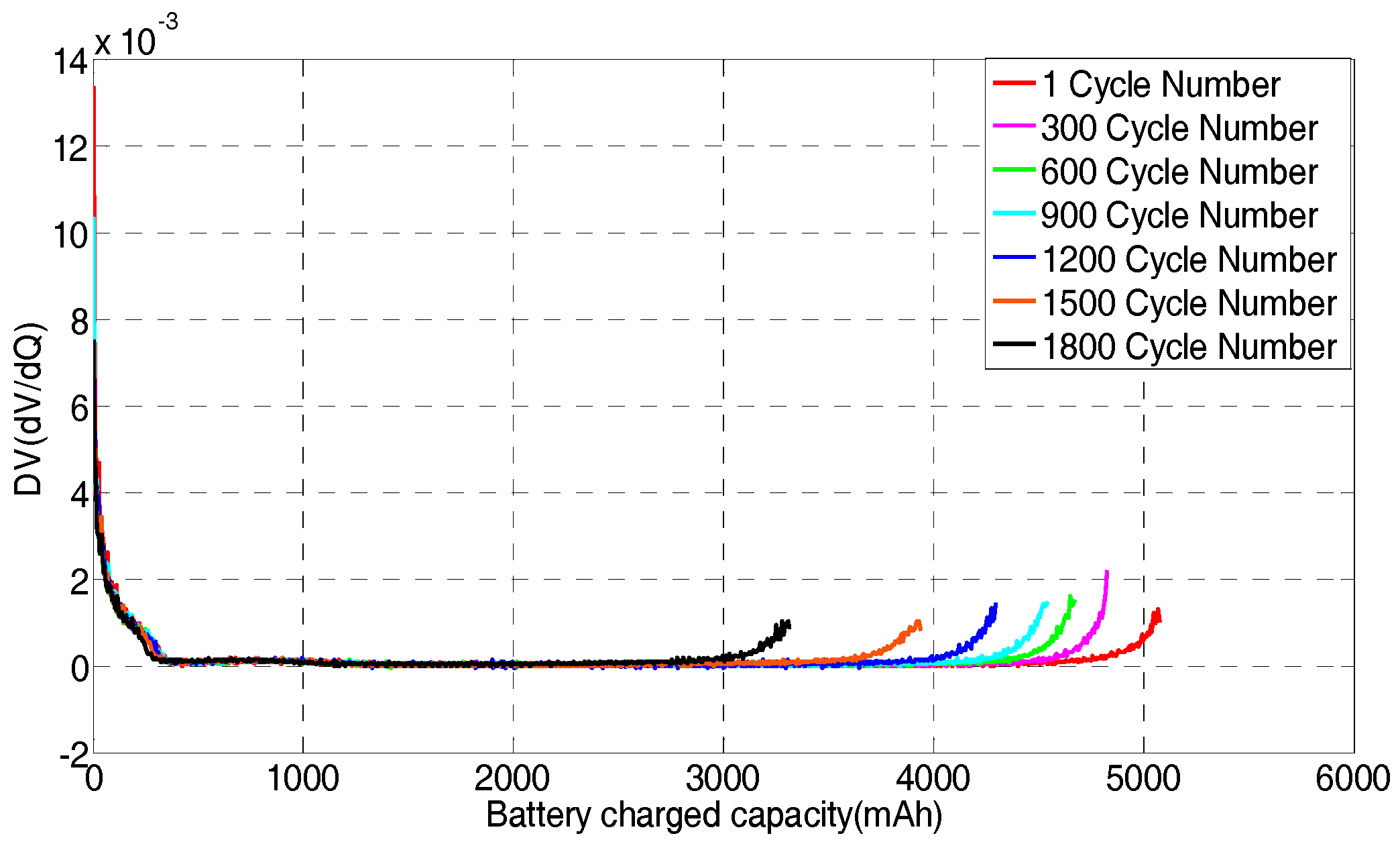
Based on the analysis stated above, the characteristics of battery regression not only relate to the terminal voltage during the charging process, but also correlate with the charging capacity. In this paper, both charge voltage and charge capacity are considered. The features of the terminal voltage curves and the characteristics of the DV during the charging process under different cycle numbers are employed as training data for the battery regression model. As shown in Figure 5, the DV in the two charge terminals obviously changes. In the initial charging stage, although the DV has noticeably changed, no clear distinction exists among different cycle numbers, as shown in Figure 6a. Thus, in this process, the DV is inadequate when considered as the battery’s regression feature value. On the other hand, in Figure 6b, the DV changes distinctly during the charging process under different cycle numbers. Therefore, it can be said that the DV can effectively describe battery health conditions.
As shown in Figure 4, the battery charging capacity is clearly only 80% of the rated capacity after 1500 cycles and, thus, the EOL number of the battery is determined. Next, the actual cycle number of the battery will be predicted by the SVM model.
3. Algorithm Introduction and Data Analysis
The SVM was first proposed by Vapnik and Corinna Cortes [33], and has been extensively applied to nonlinear and high-dimension pattern recognition problems. In the machine learning area, the SVM algorithm has been investigated to realize data classification and regression analysis [34,35,36]. Generally, the SVM algorithm has been widely employed to build system models using training input and an output dataset. The training data can be set as follows:
where is a D-dimensional input dataset, is the output dataset, and is the number of sample points. The main purpose of the training process is to find an appropriate regression function to obtain the least difference between the function’s output and actual values. For a linear system, the SVM training process can be described as:
where is a dot product, and are the vector parameter and the regression parameter, respectively. is our goal function and its maximum deviation from all training data is less than a user-defined value and needs to remain as flat as possible.
Considering the fitting error in high dimensions, the so-called slack factors and are herein proposed [37]. Thus, the training process can be turned into an optimization problem:
where is a penalty factor and is more than zero, which reflects the degree of attention paid to spatial outliers. Normally, the larger is, the more attention will be paid to those outliers. Due to the complex calculation process, directly solving the problem is generally avoided. The parameter is a linearly-insensitive loss function [38]. According to the duality principle, Equation (5) can be formulated by combining Equations (3) and (4):
where and are Lagrangian multipliers. Now, the computational process can be transformed into a convex programming problem. Hypothesizing that and are the optimal solutions, the optimal results and can be calculated as follows:
where and are both supported vectors, which are divided into two categories randomly. is the number of support vectors.
In fact, most problems show nonlinear characteristics in practical applications. To solve them, a mapping function is applied to transfer data to a high-dimension space, thereby realizing the linear regression. More information on the mapping process can be found in [39]. In the high-dimension space, a kernel function can be introduced to replace the inner product of the linear problem. In this paper, the kernel function is a radial basis function (RBF):
where is the kernel center and is the function width parameter, which restricts the range of the function radial. Moreover, is introduced to the RBF kernel function and has the same function as a penalty factor. When establishing models according to the SVM algorithm, first, we need to search for the optimal parameters and based on the cross-validation method, and then train the models with the optimal parameters. Normally, when the performances of the models are satisfactory, these parameter combinations, with a smaller penalty factor, are preferred in order to reduce the time for calculation. In addition, there is a large difference in the final model precision and computational expense if we use different cross-validation methods, regardless of what the training sample is. Currently, there are three types of cross-validation methods: leave group out cross-validation (LGOCV), K-fold cross-validation (K-fold CV), and leave one out cross-validation with the repeating K-fold cross-validation method [28,40]. The first two types are low cost when used to process masses of data, making them the most frequently-used candidates in SVM cross-validation. The last one has an advantage in terms of modeling smaller amounts of data; however, since it validates each pair of data in the sample, the training cost is high. For the battery degradation model, abundant sample points are acquired by testing the battery offline. Therefore, the K-fold CV method is applied in this paper to train the battery model. The K-fold CV method divides the raw battery data into groups (often equally), and one subset data is a validation set, while the rest of the groups of data are used as the training set. Therefore, the training model can be divided into modules. Then the average accuracy rate is used as the performance index of the K-fold CV classification. The default value of is usually five. In our battery model, the training samples are evenly classified into five parts and each part includes 36 samples. Optimal parameters and are obtained using the grid search algorithm in each training process. The relevant literature shows that a grid search performed in an exponential way not only reduces the time for calculation, but also tends to find the optimal value more easily [37,38]. The parametric form and range of the grid search are as follows:
Optimal and are used as limiting parameters for final model training and an optimal separating hyperplane is found in the high-dimensional characteristic space in order to establish the SVM model, which is similar to a linearly-separable SVM. Lagrangian multipliers are also introduced to transform the problem into a quadratic programming type. Since is the positive definite kernel, the problem is a convex quadratic programming one with an optimal solution. The final optimal regression function can be written as:
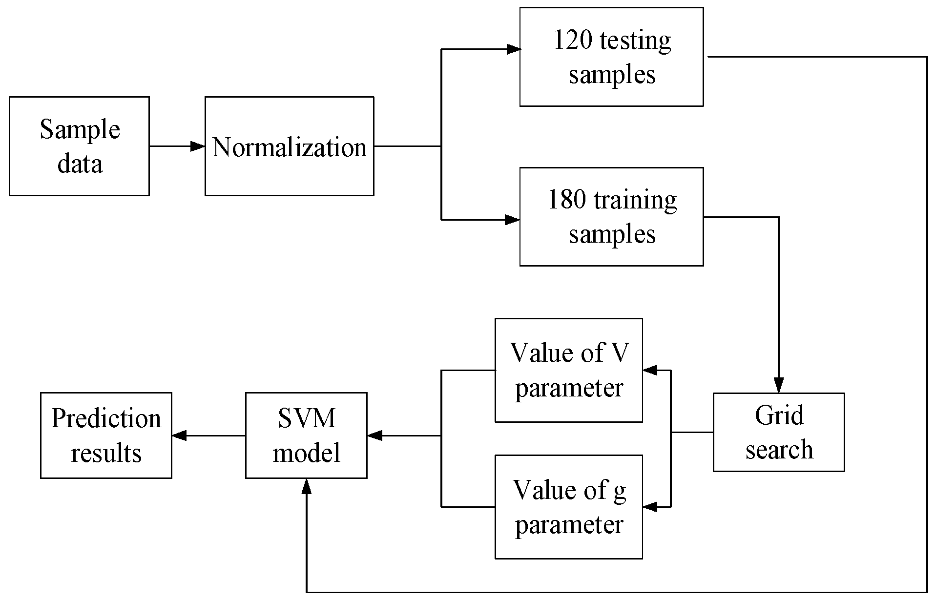
The procedures for building the battery regression model are completed based on a third toolbox under MATLAB, named libsvm [41], and the flow chart of the SVM application is shown in Figure 7. The 300 datasets are chosen from 1500 cycles of sample data, in which 60 percent of the data is used as training samples and the remaining data are the testing samples. The grid search algorithm is employed to obtain parameters and during the process of building the model. The SVM model of battery regression is completed based on and . Then, the remaining 120 datasets are applied to verify the results of the SVM model. Finally, the algorithms can determine the prediction results based on the SVM model.
4. Algorithm Application and Result Analysis
4.1. Data Analysis
In our research, the DVs and the terminal voltages under different cycle numbers are regarded as the training data for the SVM to build the estimation model. The battery actual useful life is 1500 cycles, as shown in Figure 8. Based on the cycle test, the battery charging voltage profiles possess obvious differences from the 400th sampling point. Therefore, the sampling point is regarded as the initial point and recorded in the BMS. After an interval of 100 sampling points, the terminal voltage is considered as the second point, which is also recorded in the BMS. The first equals the difference between the second point and the initial point. The second and third values are calculated in the same way. Finally, the fourth is defined as the difference between the charge cut-off voltage of 3.65 V and that of the 700th sampling point. In the cycle test, the sampling cycle interval is set as 5 s and, thus, the 400th sampling point means a voltage measurement of 2000 s. The extraction method of is similar to that of . During the RUL estimation process, the BMS only needs to record the corresponding sampling point data, thereby saving a large amount of storage space. In this paper, there exist eight variables that need to be determined in total, which can be described as .
In practical operation, the charge process can be divided into two cases: (1) incomplete sampling data, and (2) full sampling data. In the first case, supposing the charge area does not enter the 400th sampling point during an incomplete charge cycle, it is obvious that the battery degradation model cannot acquire enough characteristic data and, thus, the model cannot update the cycle number. Hence, the battery RUL for the EV is unchanged, making it the same as the previous RUL. In addition, even if the charge area enters the sampling field, the charge terminal voltage does not reach the cut-off voltage of 3.65 V. In this scenario, the sampling data is still regarded as invalid. For the sake of accuracy, the RUL can only be estimated under a complete charge cycle. In the second case, the available sampling data refers to a complete charge cycle, or the sampling start point is less than the 400th sampling point. Based on the extraction method of feature values, the battery degradation model can capture enough input, which means that eight characteristic values can be obtained. In this manner, RUL estimation based on the proposed algorithm can be achieved.
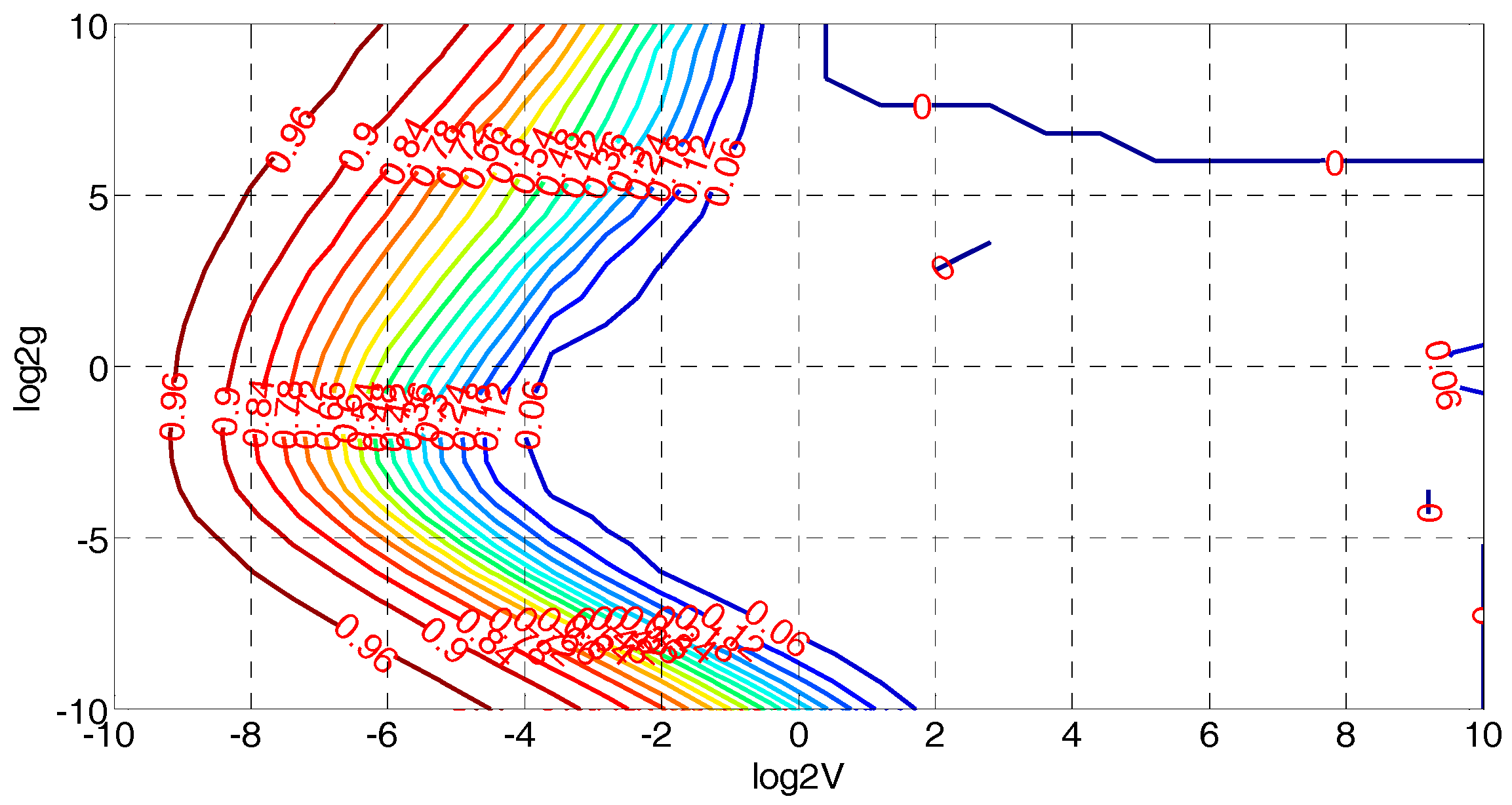
The SVM model is established using the sample data obtained by the mentioned method. The training data is divided into five folds (). Then five cross-parameter optimization processes are carried out by a grid search algorithm. The grid search algorithm is an efficient parameter search strategy for the SVM parameters. The algorithm implements a fitting method, by which the parameter grid is developed between the upper bounds and lower bounds of and . This enables searching over any sequence of parameters. Based on the fitting value, the parameters are described in Figure 9 and Figure 10. The mean square errors (MSEs) of different combinations are compared with each other to accelerate the calculation speed. According to the aforementioned principle of parameter selection, when different parameter combinations have the same least MSE, the parameters with larger values are preferred. For this battery regression model, shown in Figure 9, different parameters of least MSE can be easily obtained by the contour map. In this paper, 300 datasets are applied to build the battery degradation model and the accuracy of this model is more than 96%, as shown in Figure 10. Figure 11 shows the changing trend of the MSE with the parameters of the grid search process. Normally, the MSE decreases when increases and decreases. In addition, there is a trade-off between the number of support vectors and model precision. Meanwhile, the number of support vectors falls as increases, and when reaches a certain value, MSE will stop decreasing. In our model, is 588.1336 and equals 0.14359 based on a variety of training and overall consideration.
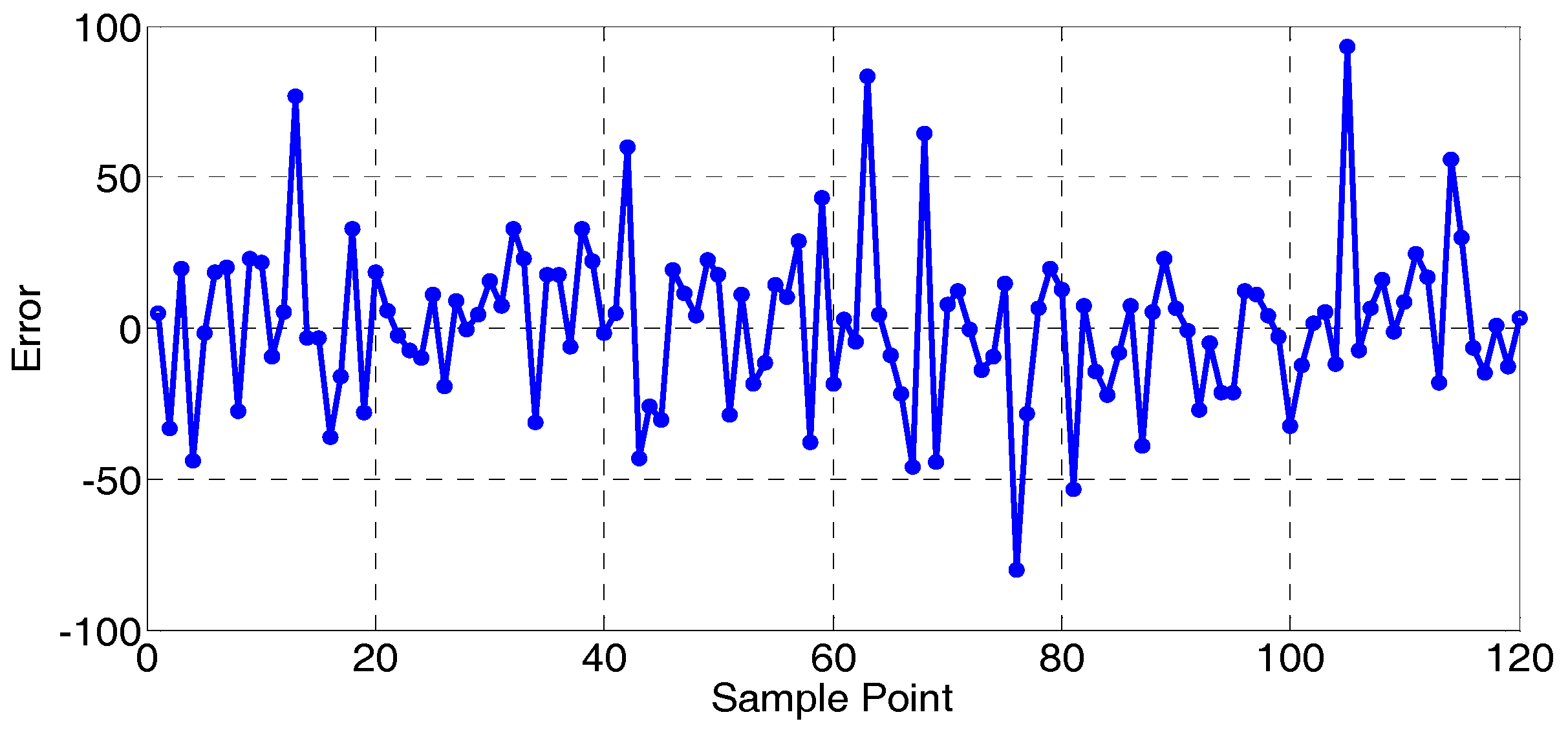
4.2. Model Setup and Analysis
According to the 1500 valid datasets, which are extracted from battery test data, each dataset contains eight training values. In this research, 300 of the 1500 sets of data (with an interval of 5) are chosen. Sixty percent of the datasets have been employed to build the model and the remaining datasets are used to verify the test results of the battery regression model. The comparison results of the predicted and actual data are shown in Figure 11. It is evident that all of the points are evenly distributed amongst 1500 cycles and the predicted values are consistent with the actual values, except for a few outliers close to 50 cycles; hence, the model’s correctness can be verified. The detailed error of the model is shown in Figure 12, from which it can be observed that the maximum value of error is 76. Thus, it implies that the RUL can be predicted with a reasonable accuracy. In addition, the MSE is 333.72 and the square correlation coefficient is 0.9982. All of these data indicate the model of battery regression is relatively accurate. We compared the SVM battery degradation model with the NN battery degradation model referred in [14]. The NN model-built battery model only considers the terminal voltages, and in the SVM model, , and its variation rate are regarded as the training data. These two datasets can improve the model accuracy to a large extent. The NN model contains 40 neurons and its MSE is 1618.4, whereas the SVM model consists of 120 support vectors and its MSE is 765.13. To sum up, the SVM model exhibits higher accuracy and lower computation complexity compared with those of the NN model.
Figure 12 and Figure 13 also illustrate that variations in actual values of the test dataset are slightly larger than those of the predicted results. In particular, there exist larger errors when the cycle number is below 100. The main reasons for this can be summarized as: firstly, in the earliest testing stages, the characteristics of the battery regression are not obvious, hence, the prediction deviations will be relatively large; and, secondly, some subjective factors exist in parameter selection and data processing.
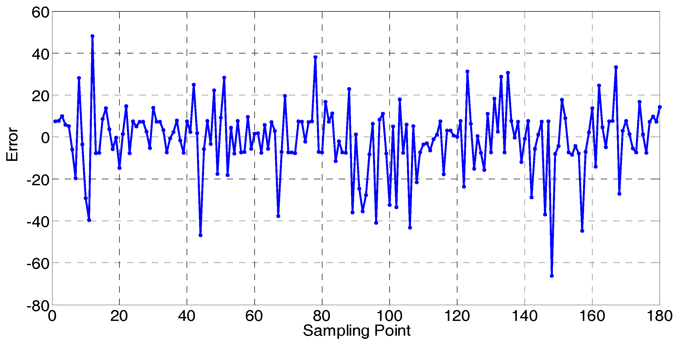
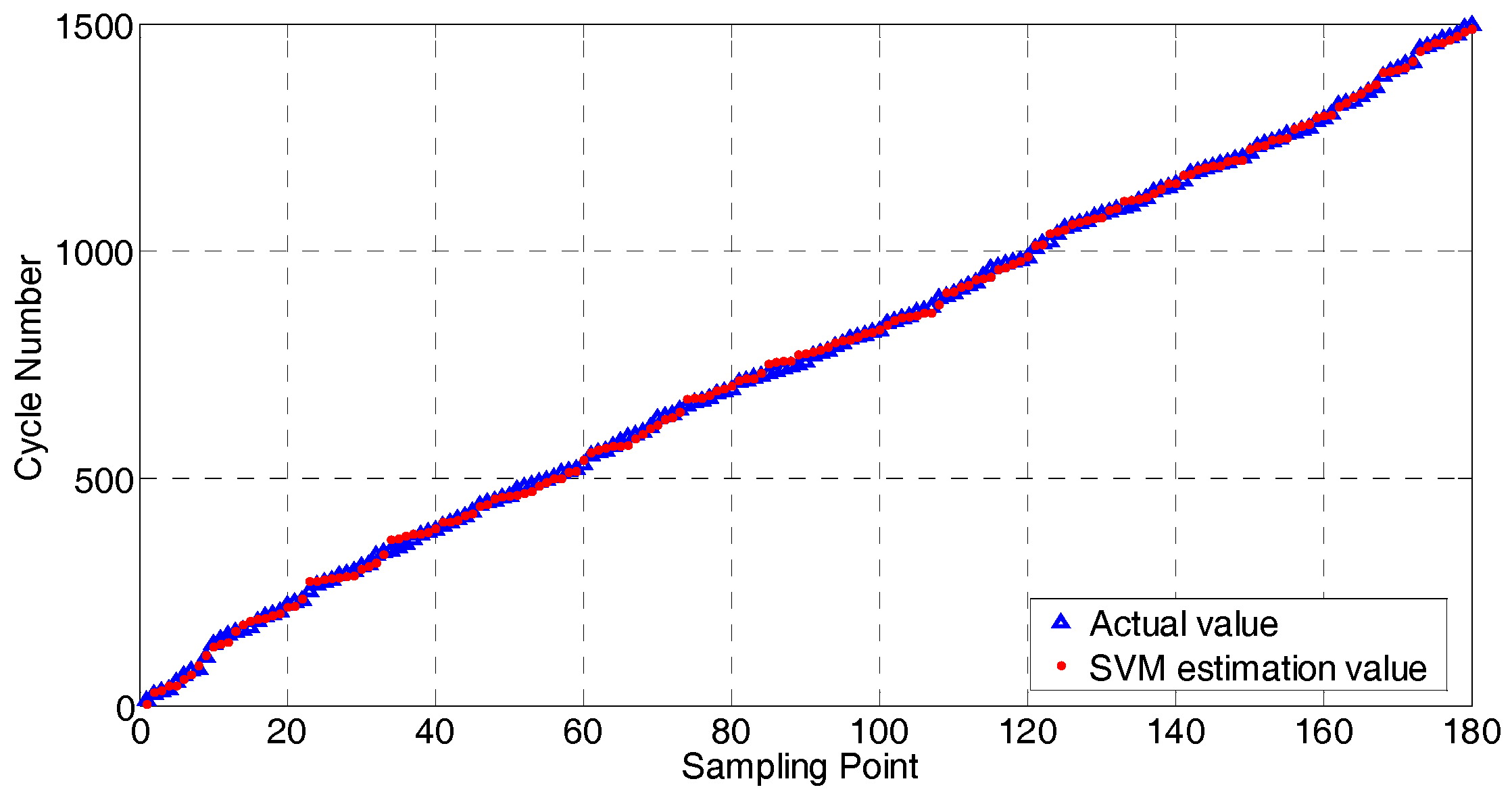
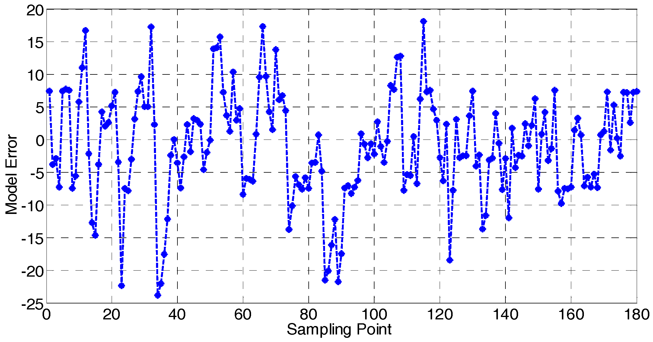
The battery regression model is verified by the remaining datasets, as shown in Figure 13. On the whole, the differences between the validation results and the actual battery cycle numbers are relatively small and can be neglected. The battery prediction error is shown in Figure 14, when the battery cycle number is less than 100. The battery regression characteristics of the DV and terminal voltage change slightly, leading to increasing preliminary prediction difficulty and decreasing the accuracy to some extent. The validation result has an MSE of 765.13 and a square correlation coefficient is 0.9959. These related coefficients indicate the SVM model of battery regression can successfully estimate battery RUL. It is necessary to mention that the model only contains 120 vectors, proving that the model is suitable for on-board prediction of the RUL of a battery in a BMS.
As shown in Figure 15 and Figure 16, 180 groups of data are selected to validate the model’s feasibility based on the trained model. The results show that when the battery begins to degrade, the voltage variation is not obvious, as only small differences exist between the characteristic values; thus, the model output error is relatively large and is around 20. When the battery degrades near the EOL, the characteristic values become more obvious, and now the model has higher precision with an output error less than 20. Hence, a conclusion can be made that the model accuracy improves with the increment of cycles.
5. Conclusions
RUL estimation is critical to battery performance optimization. In this paper, the DV and terminal voltage during the charging process are regarded as the characteristics of the battery regression. The SVM algorithm is employed to build a regression model by training these two parameters, which can predict the actual cycle number of the battery and indirectly estimate the battery RUL. The maximum error of the SVM model is 5% for the tested battery. The validation result proves that the SVM battery regression model can ensure the precision of the RUL estimation and can be finished within a limited time, thereby supplying a potential method to estimate RUL online in the BMS.
In addition, the battery RUL prediction can be affected by the battery ambient temperature, charge and discharge current rate, the discharging depth, etc. Future work will consider the influences induced by these additional factors. Research on battery degradation speed, which is related to RUL estimation, should also be conducted. Battery pack RUL estimation can also be a research direction, considering the cell-to-cell variation. Moreover, the battery regression will have an impact on the battery SOC estimation. Thus, the combined estimation of the battery regression and SOC will be comprehensively considered in the next work.
Acknowledgments
This work is supported by the project of Research and Development of Test Cycles for Chinese New Energy Vehicles–Data Acquisition in Kunming (grant no. CF2016-0163) in part; the High-Level Overseas Talents Program of Yunnan province (grant no. 10978196) in part, the Innovation Team Program of Kunming University of Science and Technology (grant no. 14078368) in part, and the Scientific Research Start-up Funding of Kunming University of Science and Technology (grant no. 14078337) in part. The authors would like to thank them for their support and help. The authors would also like to thank the reviewers for their corrections and helpful suggestions.
Author Contributions
Xiaoyu Li and Zheng Chen conceived this paper and completed the paper writing. Xing Shu performed the battery pack test cycles experiment. Renxin Xiao and Jiangwei Shen analyzed the data. Wensheng Yan provided some valuable suggestions.
Conflicts of Interest
The authors declare no conflict of interest.
References
- Wang, Y.; Zhang, C.; Chen, Z. A method for joint estimation of state-of-charge and available energy of LiFePO4 batteries. Appl. Energy 2014, 135, 81–87. [Google Scholar] [CrossRef]
- Lu, L.; Han, X.; Li, J.; Hua, J.; Ouyang, M. A review on the key issues for lithium-ion battery management in electric vehicles. J. Power Sources 2013, 226, 272–288. [Google Scholar] [CrossRef]
- Chen, Z.; Li, X.; Shen, J.; Yan, W.; Xiao, R. A novel state of charge estimation algorithm for lithium-ion battery packs of electric vehicles. Energies 2016, 9, 710. [Google Scholar] [CrossRef]
- Berecibar, M.; Gandiaga, I.; Villarreal, I.; Omar, N.; Van Mierlo, J.; Van den Bossche, P. Critical review of state of health estimation methods of Li-ion batteries for real applications. Renew. Sustain. Energy Rev. 2016, 56, 572–587. [Google Scholar] [CrossRef]
- Wang, Y.; Chen, Z.; Zhang, C. On-line remaining energy prediction: A case study in embedded battery management system. Appl. Energy 2017, 194, 688–695. [Google Scholar] [CrossRef]
- Baumhöfer, T.; Baumhöfer, T.; Brühl, M.; Rothgang, S.; Sauer, D.U. Production caused variation in capacity aging trend and correlation to initial cell performance. J. Power Sources 2014, 247, 332–338. [Google Scholar] [CrossRef]
- Chen, Z.; Mi, C.C.; Fu, Y.; Xu, J.; Gong, X. Online battery state of health estimation based on genetic algorithm for electric and hybrid vehicle applications. J. Power Sources 2013, 240, 184–192. [Google Scholar] [CrossRef]
- Miao, Q.; Xie, L.; Cui, H.; Liang, W.; Pecht, M. Remaining useful life prediction of lithium-ion battery with unscented particle filter technique. Microelectron. Reliab. 2013, 53, 805–810. [Google Scholar] [CrossRef]
- Xing, Y.; Ma, E.W.; Tsui, K.L.; Pecht, M. An ensemble model for predicting the remaining useful performance of lithium-ion batteries. Microelectron. Reliab. 2013, 53, 811–820. [Google Scholar] [CrossRef]
- Hu, C.; Jain, G.; Zhang, P.; Schmidt, C.; Gomadam, P.; Gorka, T. Data-driven method based on particle swarm optimization and k-nearest neighbor regression for estimating capacity of lithium-ion battery. Appl. Energy 2014, 129, 49–55. [Google Scholar] [CrossRef]
- Hu, C.; Jain, G.; Schmidt, C.; Strief, C.; Sullivan, M. Online estimation of lithium-ion battery capacity using sparse Bayesian learning. J. Power Sources 2015, 289, 105–113. [Google Scholar] [CrossRef]
- Sun, B.; Jiang, J.; Zheng, F.D.; Zhao, W.; Liaw, B.Y.; Ruan, H.; Han, Z.; Zhang, W. Practical state of health estimation of power batteries based on Delphi method and grey relational grade analysis. J. Power Sources 2015, 282, 146–157. [Google Scholar] [CrossRef]
- Hu, C.; Jain, G.; Tamirisa, P.; Gorka, T. Method for estimating capacity and predicting remaining useful life of lithium-ion battery. Appl. Energy 2014, 126, 182–189. [Google Scholar] [CrossRef]
- Wu, J.; Wang, Y.; Zhang, X.; Chen, Z. A novel state of health estimation method of Li-ion battery using group method of data handling. J. Power Sources 2016, 327, 457–464. [Google Scholar] [CrossRef]
- Honkura, K.; Takahashi, K.; Horiba, T. Capacity-fading prediction of lithium-ion batteries based on discharge curves analysis. J. Power Sources 2011, 196, 10141–10147. [Google Scholar] [CrossRef]
- Wu, J.; Zhang, C.; Chen, Z. An online method for lithium-ion battery remaining useful life estimation using importance sampling and neural networks. Appl. Energy 2016, 173, 134–140. [Google Scholar] [CrossRef]
- Weng, C.; Sun, J.; Peng, H. A unified open-circuit-voltage model of lithium-ion batteries for state-of-charge estimation and state-of-health monitoring. J. Power Sources 2014, 258, 228–237. [Google Scholar] [CrossRef]
- Han, X.; Ouyang, M.; Lu, L.; Li, J.; Zheng, Y.; Li, Z. A comparative study of commercial lithium ion battery cycle life in electrical vehicle: Aging mechanism identification. J. Power Sources 2014, 251, 38–54. [Google Scholar] [CrossRef]
- Weng, C.; Cui, Y.; Sun, J.; Peng, H. On-board state of health monitoring of lithium-ion batteries using incremental capacity analysis with support vector regression. J. Power Sources 2013, 235, 36–44. [Google Scholar] [CrossRef]
- Torai, S.; Torai, S.; Nakagomi, M.; Yoshitake, S.; Yamaguchi, S.; Oyama, N. State-of-health estimation of LiFePO4/graphite batteries based on a model using differential capacity. J. Power Sources 2016, 306, 62–69. [Google Scholar] [CrossRef]
- Wang, L.; Pan, C.; Liu, L.; Cheng, Y.; Zhao, X. On-board state of health estimation of LiFePO4 battery pack through differential voltage analysis. Appl. Energy 2016, 168, 465–472. [Google Scholar] [CrossRef]
- Li, Y.; Chattopadhyay, P.; Ray, A.; Rahn, C.D. Identification of the battery state-of-health parameter from input–output pairs of time series data. J. Power Sources 2015, 285, 235–246. [Google Scholar] [CrossRef]
- Li, F.; Xu, J. A new prognostics method for state of health estimation of lithium-ion batteries based on a mixture of Gaussian process models and particle filter. Microelectron. Reliab. 2015, 55, 1035–1045. [Google Scholar] [CrossRef]
- Andre, D.; Appel, C.; Soczka-Guth, T.; Sauer, D.U. Advanced mathematical methods of SOC and SOH estimation for lithium-ion batteries. J. Power Sources 2013, 224, 20–27. [Google Scholar] [CrossRef]
- Dong, H.; Jin, X.; Lou, Y.; Wang, C. Lithium-ion battery state of health monitoring and remaining useful life prediction based on support vector regression-particle filter. J. Power Sources 2014, 271, 114–123. [Google Scholar] [CrossRef]
- Hu, X.; Jiang, J.; Cao, D.; Egardt, B. Battery health prognosis for electric vehicles using sample entropy and sparse Bayesian predictive modeling. IEEE Trans. Ind. Electron. 2016, 63, 2645–2656. [Google Scholar] [CrossRef]
- Saha, B.; Goebel, K.; Poll, S.; Christophersen, J. Prognostics methods for battery health monitoring using a Bayesian framework. IEEE Trans. Instrum. Meas. 2009, 58, 291–296. [Google Scholar] [CrossRef]
- Martínez-Morales, J.D.; Palacios-Hernández, E.R.; Velázquez-Carrillo, G.A. Modeling and multi-objective optimization of a gasoline engine using neural networks and evolutionary algorithms. J. Zhejiang Univ. Sci. A 2013, 14, 657–670. [Google Scholar] [CrossRef]
- Klass, V.; Behm, M.; Lindbergh, G. A support vector machine-based state-of-health estimation method for lithium-ion batteries under electric vehicle operation. J. Power Sources 2014, 270, 262–272. [Google Scholar] [CrossRef]
- Weng, C.; Sun, J.; Peng, H. Model parametrization and adaptation based on the invariance of support vectors with applications to battery state-of-health monitoring. IEEE Trans. Veh. Technol. 2015, 64, 3908–3917. [Google Scholar] [CrossRef]
- Liu, D.; Zhou, J.; Pan, D.; Peng, Y.; Peng, X. Lithium-ion battery remaining useful life estimation with an optimized Relevance Vector Machine algorithm with incremental learning. Measurement 2015, 63, 143–151. [Google Scholar] [CrossRef]
- Wang, D.; Miao, Q.; Pecht, M. Prognostics of lithium-ion batteries based on relevance vectors and a conditional three-parameter capacity degradation model. J. Power Sources 2013, 239, 253–264. [Google Scholar] [CrossRef]
- Cortes, C.; Vapnik, V. Support-Vector Networks. Mach. Learn. 1995, 20, 273–297. [Google Scholar] [CrossRef]
- Smola, A.J.; Schölkopf, B. A tutorial on support vector regression. Stat. Comput. 2004, 14, 199–222. [Google Scholar] [CrossRef]
- Rivas-Perea, P.; Cota-Ruiz, J.; Rosiles, J.-G. A nonlinear least squares quasi-Newton strategy for LP-SVR hyper-parameters selection. Int. J. Mach. Learn. Cybern. 2014, 5, 579–597. [Google Scholar] [CrossRef]
- Noble, W.S. What is a support vector machine? Nat. Biotechnol. 2006, 24, 1565–1567. [Google Scholar] [CrossRef] [PubMed]
- Wang, Z.Q.; Sun, X.; Zhang, D.X.; Li, X. An optimal SVM-based text classification algorithm. In Proceedings of the 2006 International Conference on Machine Learning and Cybernetics, Dalian, China, 13–16 August 2006. [Google Scholar] [CrossRef]
- Wang, L. Support Vector Machines: Theory and Applications; Springer Science & Business Media: New York, NY, USA, 2005; ISSN 1434-9922. [Google Scholar]
- Suykens, J.A.K.; Vandewalle, J. Least squares support vector machine classifiers. Neural Process. Lett. 1999, 9, 293–300. [Google Scholar] [CrossRef]
- Kuhn, M.; Johnson, K. Applied Predictive Modeling; Springer: Berlin, Germany, 2013; ISBN 978-1-4614-6848-6. [Google Scholar]
- Chang, C.-C.; Lin, C.-J. LIBSVM: A library for support vector machines. ACM Trans. Intell. Syst. Technol. TIST 2011, 2, 27. [Google Scholar] [CrossRef]
Figure 1.
Battery test schedule.

Figure 2.
Batteries’ charge terminal voltages under different cycle numbers.

Figure 3.
Battery charge capacity in different cycle numbers.
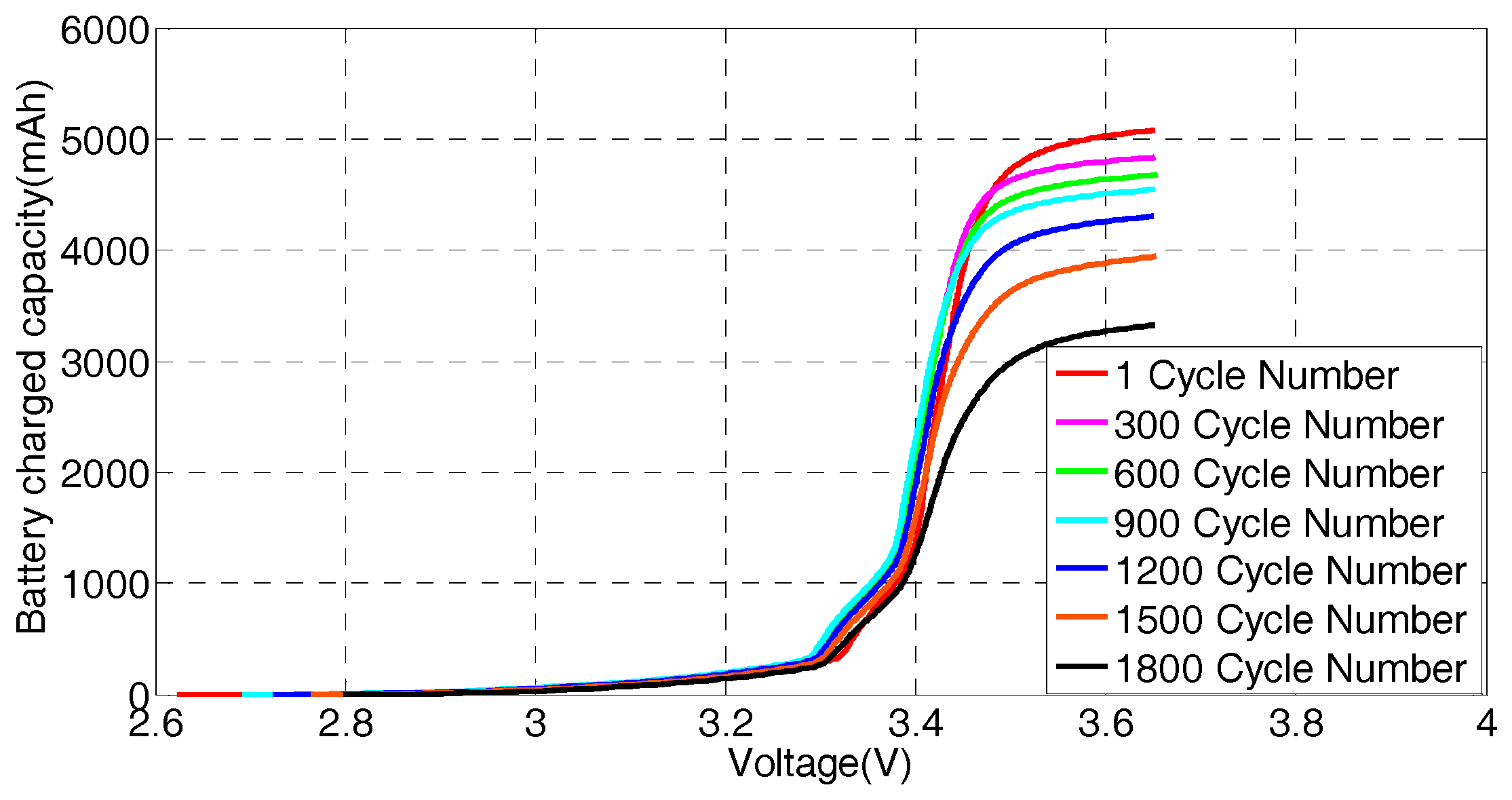
Figure 4.
Voltage curves: (a) charge plateau region voltage; and (b) terminal voltage region.

Figure 5.
The differential voltage under different cycle numbers.

Figure 6.
(a) Differential voltage during the initial charging process; and (b) differential voltage at the end of the charging process.
Figure 6.
(a) Differential voltage during the initial charging process; and (b) differential voltage at the end of the charging process.
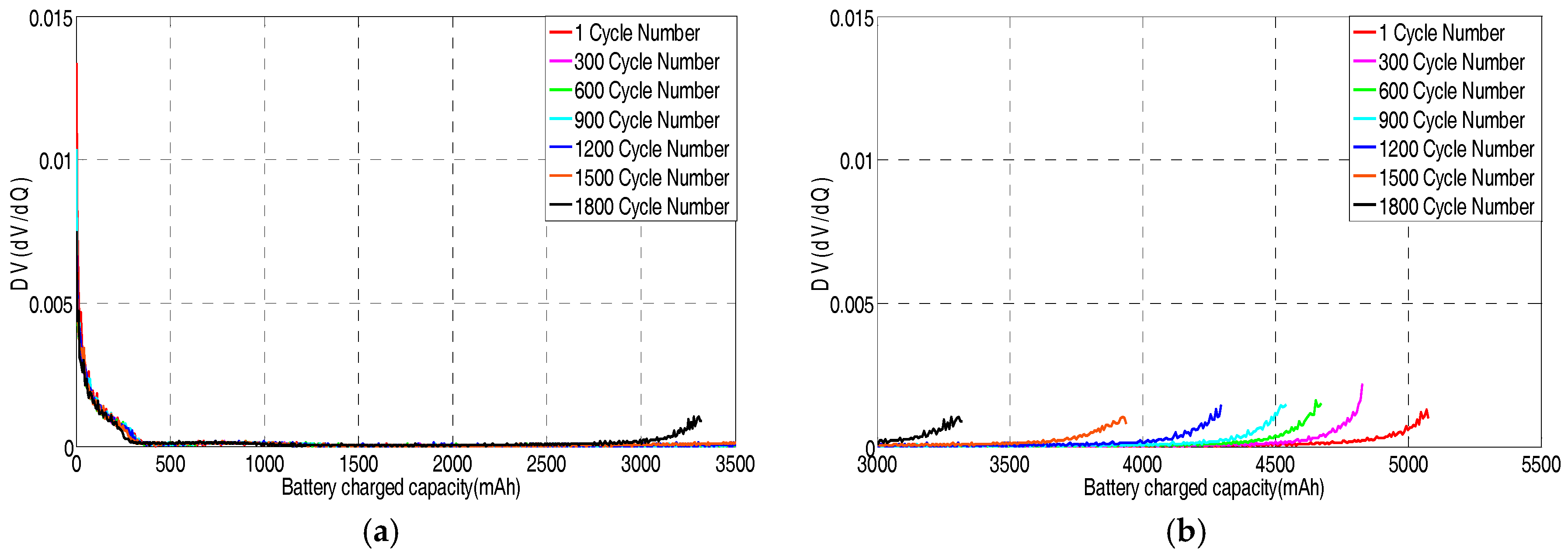
Figure 7.
The process of applying the SVM model.

Figure 8.
The SVM training data: (a) the specific delta V data; and (b) the specific delta DV data.

Figure 9.
The relationship between MSE and parameters V, g.
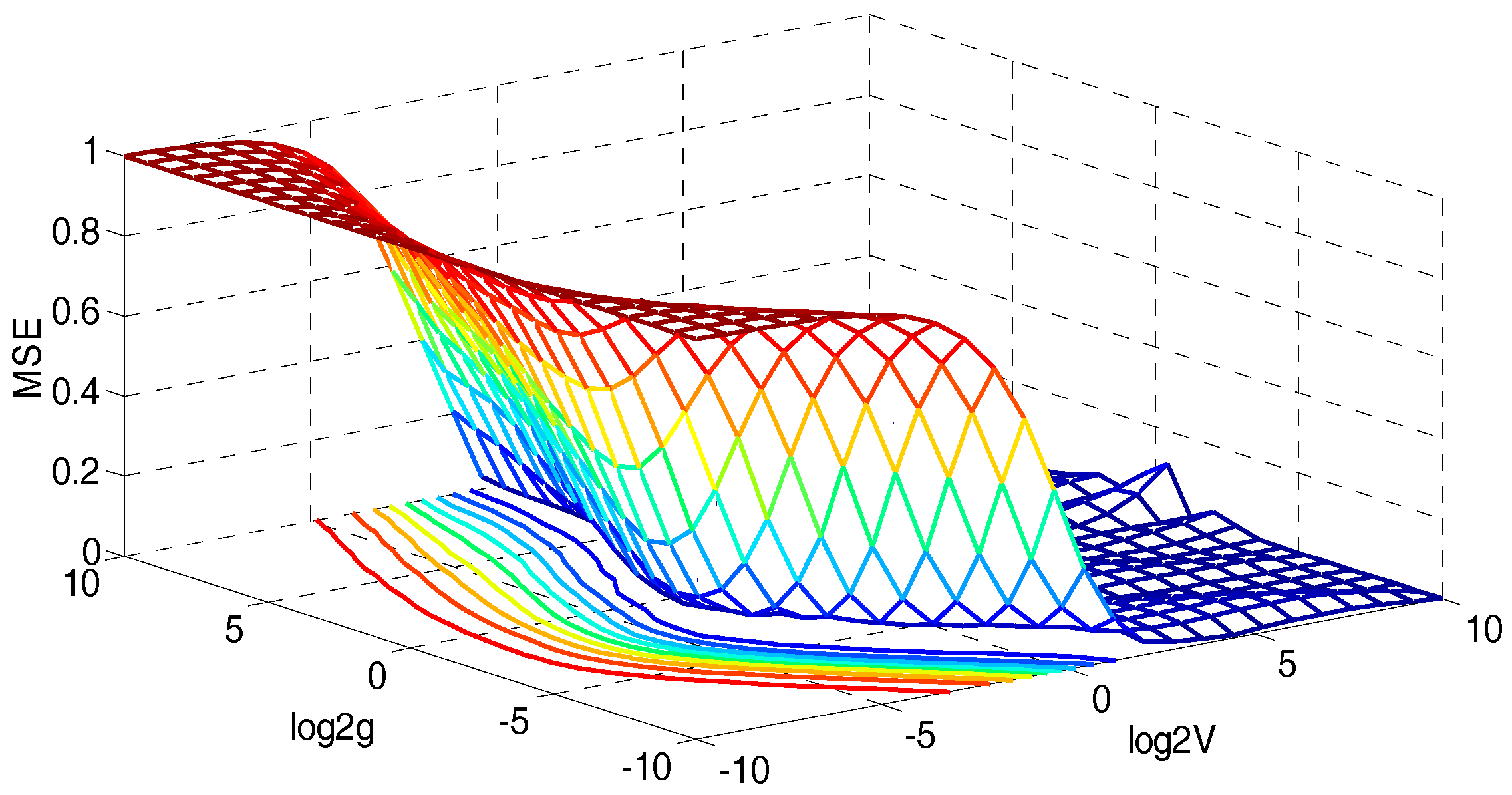
Figure 10.
The contour of the optimal parameters.

Figure 11.
The estimation result of the SVM model.
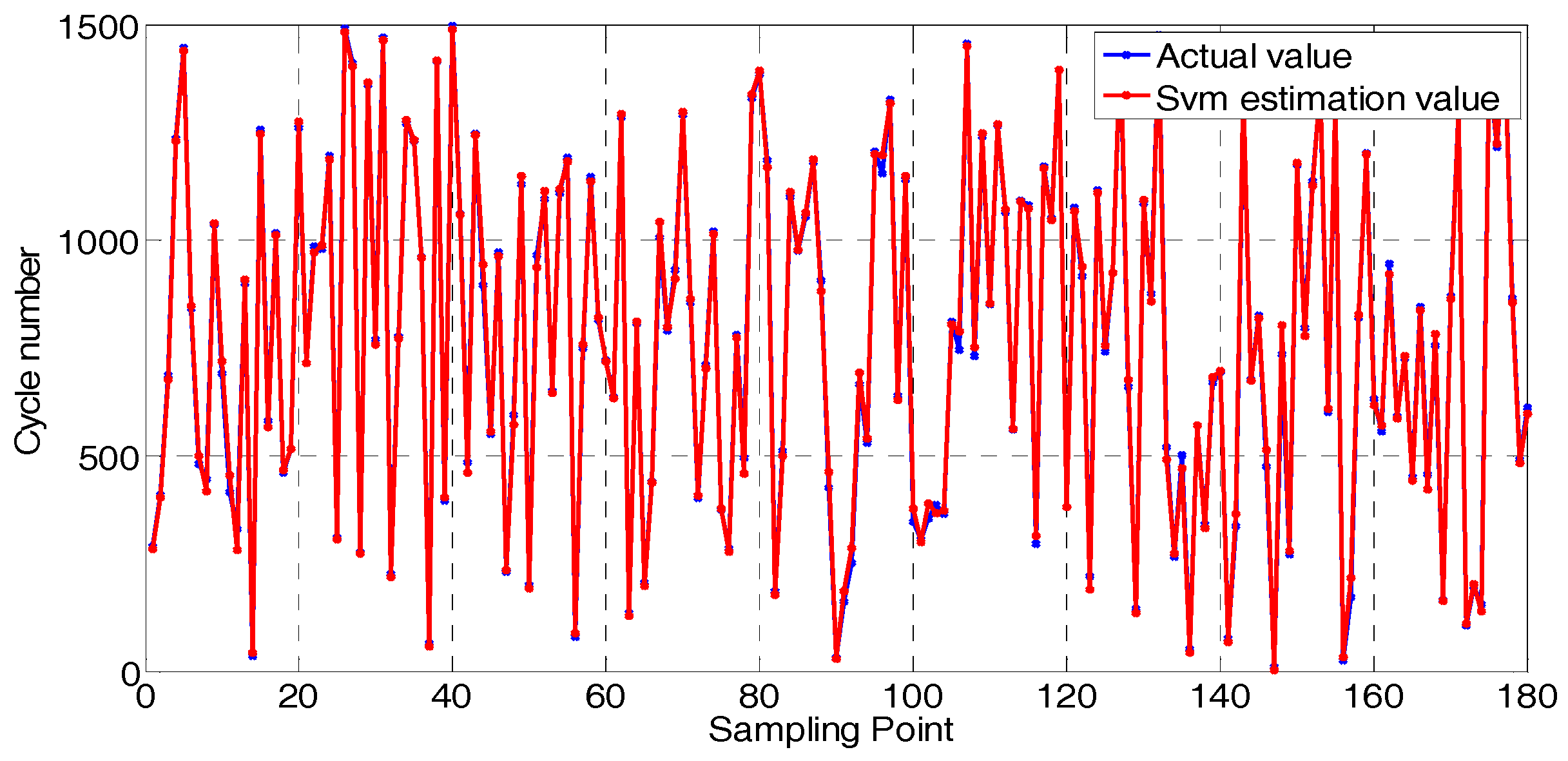
Figure 12.
The analysis of the SVM model estimation error.

Figure 13.
The cross-validation of the battery regression model.
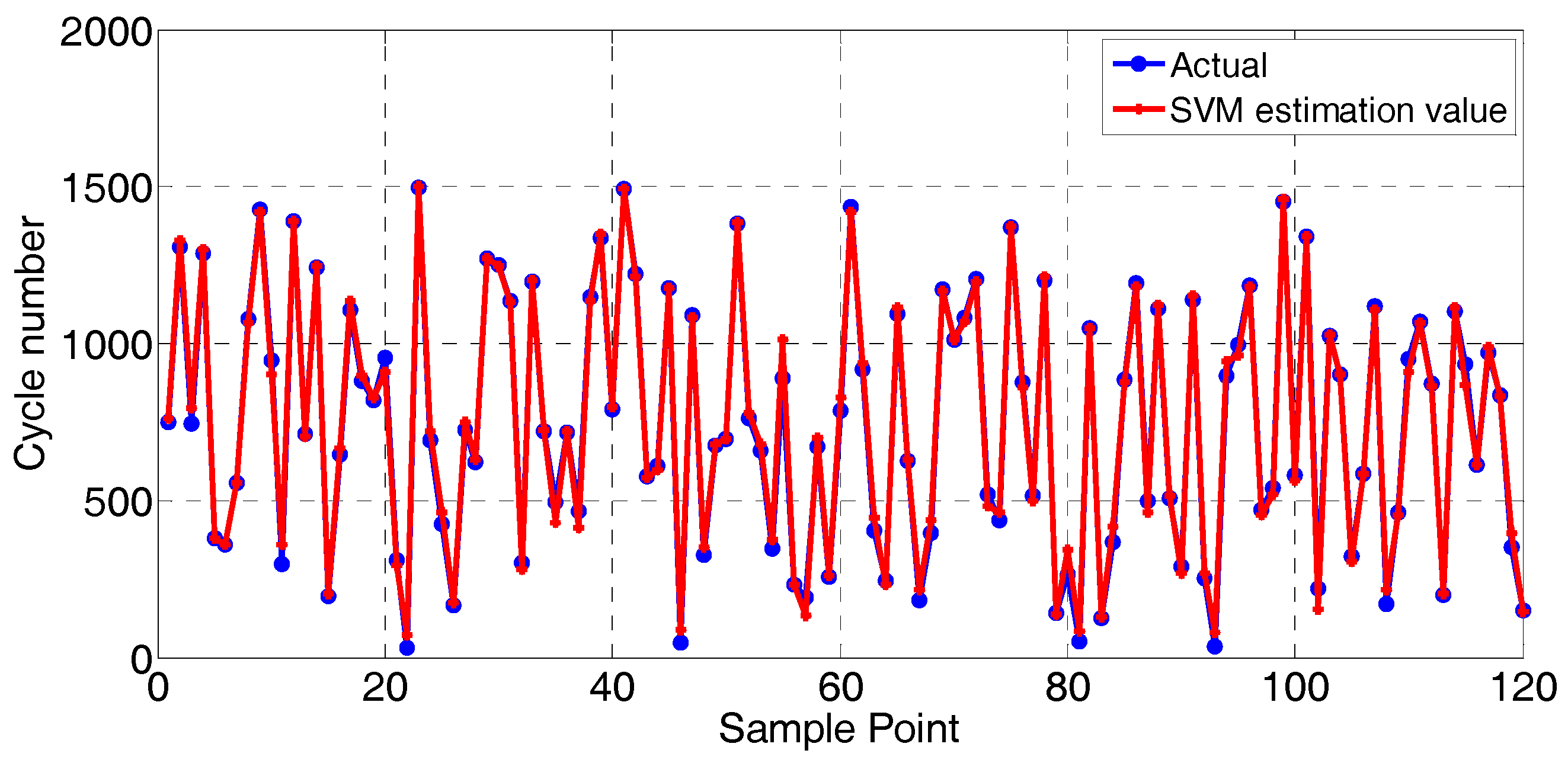
Figure 14.
The cross-validation analysis.

Figure 15.
The result of the SVM model.

Figure 16.
The error of the SVM model.

© 2017 by the authors. Licensee MDPI, Basel, Switzerland. This article is an open access article distributed under the terms and conditions of the Creative Commons Attribution (CC BY) license (http://creativecommons.org/licenses/by/4.0/).
Share and Cite
MDPI and ACS Style
Li, X.; Shu, X.; Shen, J.; Xiao, R.; Yan, W.; Chen, Z. An On-Board Remaining Useful Life Estimation Algorithm for Lithium-Ion Batteries of Electric Vehicles. Energies 2017, 10, 691. https://doi.org/10.3390/en10050691
AMA Style
Li X, Shu X, Shen J, Xiao R, Yan W, Chen Z. An On-Board Remaining Useful Life Estimation Algorithm for Lithium-Ion Batteries of Electric Vehicles. Energies. 2017; 10(5):691. https://doi.org/10.3390/en10050691
Chicago/Turabian StyleLi, Xiaoyu, Xing Shu, Jiangwei Shen, Renxin Xiao, Wensheng Yan, and Zheng Chen. 2017. "An On-Board Remaining Useful Life Estimation Algorithm for Lithium-Ion Batteries of Electric Vehicles" Energies 10, no. 5: 691. https://doi.org/10.3390/en10050691
Note that from the first issue of 2016, this journal uses article numbers instead of page numbers. See further details here.