
Multi-Objective Optimization of Hybrid Renewable Energy System Using an Enhanced Multi-Objective Evolutionary Algorithm

College of Information Systems and Management, National University of Defense Technology, Changsha 410073, China
*
Author to whom correspondence should be addressed.
Energies 2017, 10(5), 674; https://doi.org/10.3390/en10050674
Submission received: 1 March 2017
/
Revised: 26 April 2017
/
Accepted: 5 May 2017
/
Published: 11 May 2017
(This article belongs to the Section F: Electrical Engineering)
Abstract
:Due to the scarcity of conventional energy resources and the greenhouse effect, renewable energies have gained more attention. This paper proposes methods for multi-objective optimal design of hybrid renewable energy system (HRES) in both isolated-island and grid-connected modes. In each mode, the optimal design aims to find suitable configurations of photovoltaic (PV) panels, wind turbines, batteries and diesel generators in HRES such that the system cost and the fuel emission are minimized, and the system reliability/renewable ability (corresponding to different modes) is maximized. To effectively solve this multi-objective problem (MOP), the multi-objective evolutionary algorithm based on decomposition (MOEA/D) using localized penalty-based boundary intersection (LPBI) method is proposed. The algorithm denoted as MOEA/D-LPBI is demonstrated to outperform its competitors on the HRES model as well as a set of benchmarks. Moreover, it effectively obtains a good approximation of Pareto optimal HRES configurations. By further considering a decision maker’s preference, the most satisfied configuration of the HRES can be identified.
1. Introduction
The increasing consumption of fossil fuels coupled with environmental degradation has resulted in the growth of eco-friendly renewable energy resources [1]. The hybrid renewable energy system (HRES) that integrates various renewable energy resources together has become increasingly popular [2]. The optimization of HRES is a multi-objective problem (MOP) in nature. To be specific, multiple objectives have to be considered simultaneously [3] such as minimizing the lifetime system costs, the carbon emissions, maximizing the system reliability, and the utilization of renewable energies.
Given multifarious variables and non-linear models, the single-objective algorithms are hard to find the global optimum. In recent decades, multi-objective optimization methods, due to their good performance on obtaining the trade-offs for MOPs, have been extensively applied to the optimal design of HRESs [4]. The most popular approach proposed to solve these kinds of problems is a multi-objective evolutionary algorithm (MOEA), which has been used to design or schedule many hybrid power systems [1,5,6,7,8,9]. For example, Dufo-López and Bernal-Agustín [7] applied the strength Pareto evolutionary algorithm (SPEA) to optimize the cost, pollution and unmet load of the HRES. In [10], the non-dominated sorting genetic algorithm (NSGA) [11] was introduced to the optimization of HRES with two objectives, i.e., minimizing the total cost and pollutant emissions. Following those Pareto-based algorithms, the MOEA based on decomposition (MOEA/D) [12] was also used in this research area for computational efficiency and scalability. It has been applied in [13] to optimize an HRES in which the cost, CO2 and SO2 emissions are minimized and the output power is maximized.
However, most of the existing studies tend to merely consider renewable resources as an isolated-island mode (the HRES responds to the load demand on itself). In fact, the HRES can also connect to the power grid (that is, the HRES exchanges power with the public grid [14,15]), which can further enhance the reliability and the economic benefit of HRES. In this study, the multi-objective design of HRES that operates in both isolated-island and grid-connected modes is modelled and simulated. The contributions are that (i) a comprehensive set of components are considered in the design of HRES. Taking the batteries as an example, the shortened lifespan of batteries resulted from the frequent charge–discharge cycles is calculated; (ii) this paper describes the HRES that can operate in both isolated-island and grid-connected modes. In addition, the optimal operational strategy for each mode is provided; and (iii) a simple yet effective algorithm, namely, MOEA/D with a localized penalty-based boundary intersection (LPBI) method (denoted as MOEA/D-LPBI) is proposed for the multi-objective design of HRES in both modes. The MOEA/D-LPBI can eliminate the need of penalty value setting in the original MOEA/D-PBI, and significantly outperforms MOEA/D-PBI on both benchmarks and the multi-objective design of HRES.
The remainder of this paper is presented as follows. The optimization model and the control strategy of HRES are presented in Section 2. Section 3 introduces the LPBI method and the derived algorithm, MOEA/D-LPBI. Section 4 examines the performance of MOEA/D-LPBI on benchmarks and demonstrates its performance on the design of HRES. Section 5 concludes the paper and identifies future studies.
2. Mathematical Model of the HRES
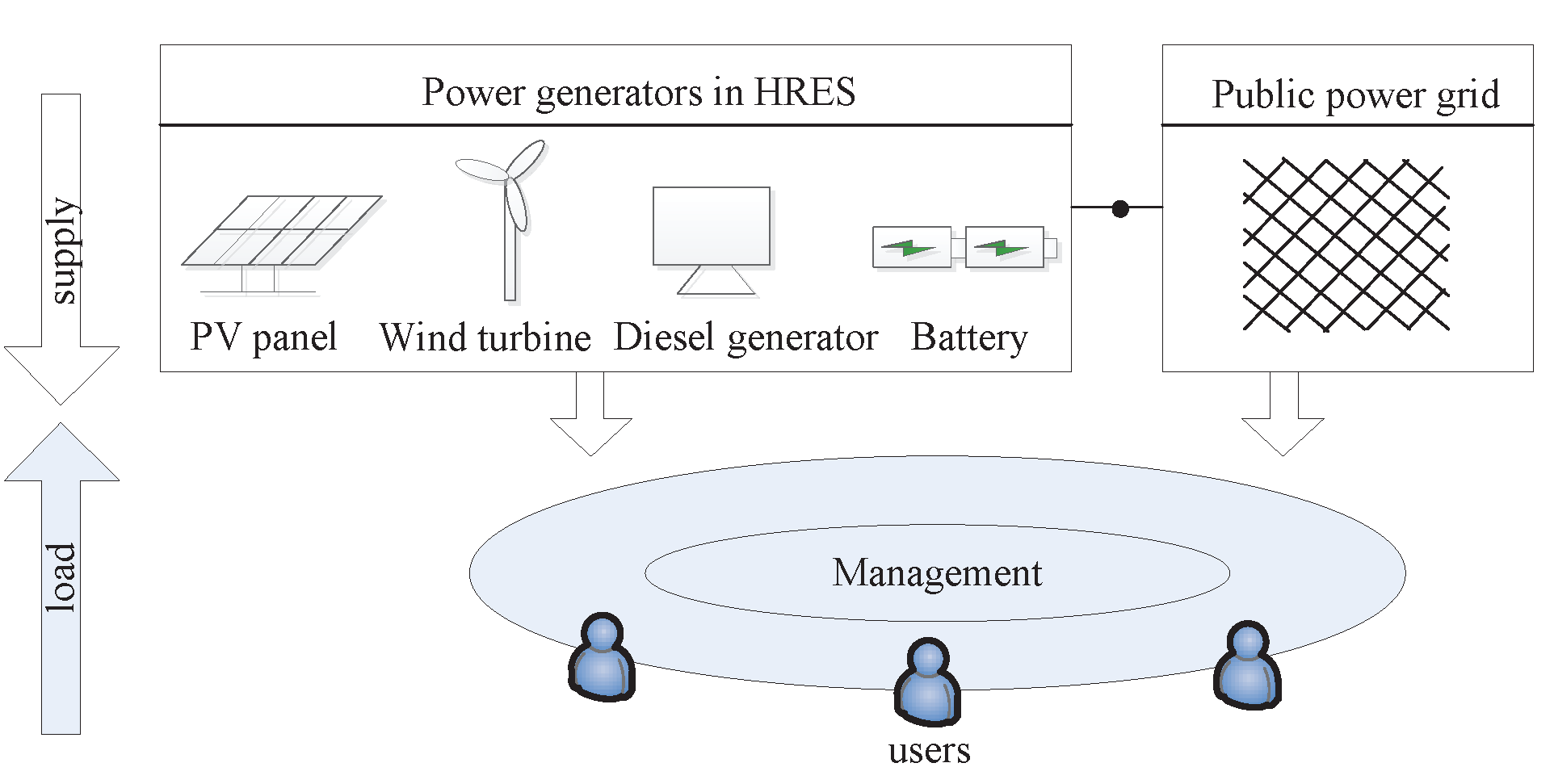
In general, an HRES consists of photovoltaic (PV) panels, wind turbines, the battery storage, diesel generators and some accessory devices. The considered HRES in which the power grid can be also included is illustrated in Figure 1. The details about the optimization model and the operational mechanism are elaborated in the following subsections.
2.1. Optimization Model
As a piece of important generating equipment, the PV panel has been widely used because of its safety and no pollution. Assuming that the PV array combines of PV panels in series and strings in parallel, the maximum output power can be calculated as Equation (1) [16]:
where the factor takes into account the losses of power due to shadows, dirt, etc. The total number of PV units () is available by multiplying . The calculation method to obtain the electric current and the voltage is employed from the previous work [17].
The wind turbine consists of the wind tower and the generator, whose output power can be calculated as follows [18]:
with:
where is a coefficient obtained by the maximum wind power dividing the actual power output, is the air density, is the cross section of the rotor, and denotes the rated power of the wind turbine. , and are the cut-in, the rated and the cut-off wind velocity, respectively. In addition, the wind velocity v at the (actual) height of is converted by the anemometer data () at the reference height of as Equation (3). Note that the height of wind tower is retained within .
The batteries are frequently applied in an HRES as the storage device. The quantity of electric charge and discharge is dependent on not only the load demand but also the state of charge (). The of the battery storage at the simulation time t is obtained by Equation (4):
where is the input/output power (positive during charging and negative during discharging) of batteries. is each simulation time step that is assumed to be an hour. The round-trip efficiency is defined as 80% for charging and 100% for discharging models. Additionally, , and denote the number of batteries, the nominal capacity and the nominal voltage of each battery, respectively.
The battery model retains the between the lower limit () and the upper limit () to ensure safety. Correspondingly, the minimum and the maximum battery power are also defined respectively, as shown in Equations (5) and (6):
Since the number of the charge–discharge circles and the depth of discharge in each circle both affect the lifespan of the batteries, the “rainflow”-based method described in [7] is adopted to estimate the actual lifetime of the battery storage . When the working hours reach the longevity (), new batteries will replace those old ones.
The diesel generator usually acts as the back-up power and its fuel consumption is identified [7] as Equation (7):
where and are the rated and actual output power, respectively. Note that the latter is not allowed to be larger than the former. and are coefficients of fuel consumption.
In addition to the above components, some accessory devices, such as the inverter and the rectifier, are also included. Their efficiencies are 90% and 95%, respectively.
As for the objectives in this HRES, it is always expected that the system cost and the output pollution can be minimized. In addition, the load demand can be met. Due to the fact that the HRES can be in either grid-connected mode or isolated-island mode, the optimal design of HRES could be different. Specifically, for the isolated mode, the cost of system (), fuel emissions () and the probability of unsatisfying the load demand () are to be minimized; for the grid-connected mode, the cost of system (), fuel emissions () and the proportion of non-renewable energy () are to be minimized. Afterwards, we present the definitions of these objectives.
First, we assume that the lifespan of the HRES is determined by the lifetime of PV panels. Since the batteries have shorter service life and the frequent charge–discharge pattern further shortens the time, its replacement is also considered in this work. Overall, the total cost is comprised of the following:
- Payment of purchasing and installing the PV panels, wind turbines, batteries, diesel generators, inverters and rectifiers, denoted as . Among them, the cost of the wind turbines includes that of the wind generator and the tower, and the expense in tower is positively related to its height.
- Cost of repair and maintenance of the devices, denoted as .
- Expenditure on the fuel consumed through the lifespan, denoted as , which is defined by unit price () multiplying the quantity of fuel consumption ().
- Cost of replacing the old batteries with the new ones, denoted as . It is calculated by where and are the unit price of a battery and the number of replacement, respectively.
- Cost/profit of exchanging power with the public power grid (positive for buying power and negative for selling power), denoted as .
The costs considered above are indicated as Equation (8):
where is zero when the system operates in the isolated-island mode.
Second, we adopt the total amount of through the lifespan (T) to measure the pollutant emissions as occupies the largest percentage of all emissions in fuel combustion:
where is the emission factor depending upon the property of the diesel generator and is the maximum simulation time. The amount of emission accumulates every time the device is powered [19].
Third, the probability of failing to satisfy all of the load () is employed to measure the system reliability in the isolated-island mode, which is calculated by Equation (10):
with:
where the available power supply and the load demand are compared for each simulation time, and 1 is returned to (boolean variable) if the former is smaller than the latter and vice versa. Thus, refers to the proportion of hours of power shortage during the lifetime, within [0, 1].
In the grid-connected mode, is always zero since the deficit power can be bought from the power. Thus, the proportion of using non-renewable energy () is considered instead, and is defined in Equation (12):
Overall, the design of an HRES is an MOP where three objectives are to be minimized as shown in Equation (13):
subject to:
2.2. Systematic Planning of Operation Mechanism
The energy flow in the HRES is illustrated in Figure 2 with two modes considered. Mode I is the isolated-island mode, and mode II is the grid-connected mode.
- Mode I: in this mode, the system is not connected to the power grid, thus the A module in Figure 2 is not considered. The energy produced by the PV panels and the wind turbines is directly provided for the direct-current (DC) load and flows to the alternating-current (AC) load through the inverter. If the provided energy exceeds the total demand (DC load plus AC load), the surplus energy will be saved in the battery storage after meeting the load. On the contrary, if it cannot satisfy the load demand, the batteries will discharge based on the . If there still exists unmet load, the diesel generators start as the emergency power-supply. Note that the power from the diesel generators is alternating current and the part used to supply DC load is converted by the AC-to-DC rectifier.
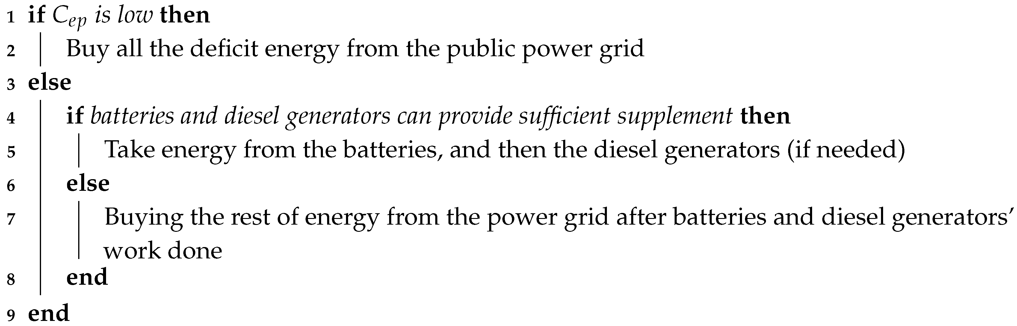
- Mode II: in this mode, when the produced renewable energy is more than the demanded quantity and the batteries have been charged to the maximum, the surplus energy will be sold to the power grid for the profit. On the contrary, if the produced energy cannot meet the load demand, the method of obtaining the supplement is determined by the electricity price (). Providing low , all of the deficit power will be bought from the public power grid and supplied to the load. On this condition, the B module does not operate. However, if the is high, first the battery storage and the diesel generators are used as supplement power. Once these devices still cannot cover the gap, the required power will be bought from the power grid. To describe it more clearly, the choosing strategy when the renewable energy is insufficient is shown in Algorithm 1.
| Algorithm 1: Decision strategy for the source of supplementing deficit energy in mode II. |
 |
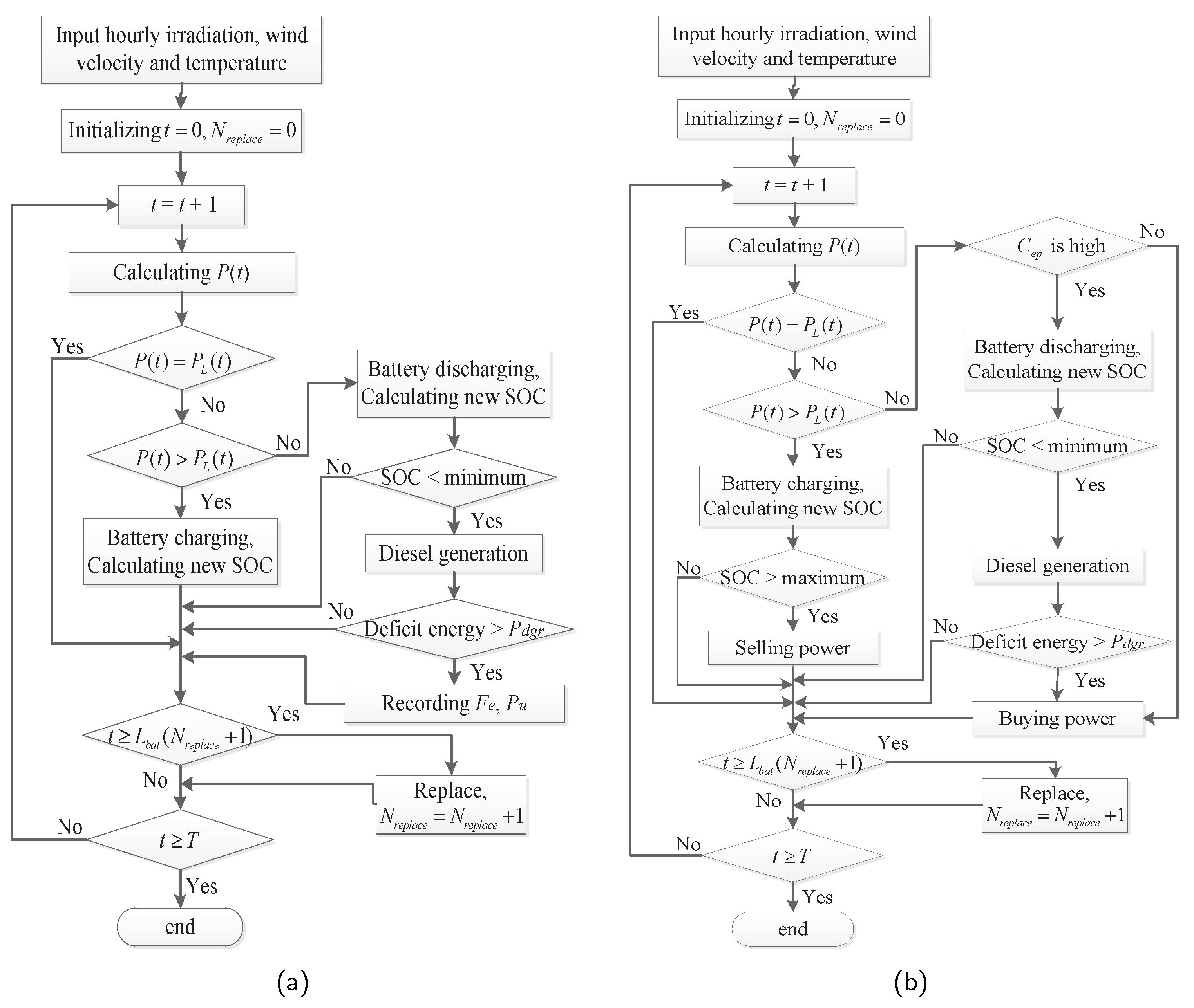
To simulate the operational process, the flowchart is shown in Figure 3. In this flowchart, and are the total power produced by renewable resources (PVs plus wind turbines) and the load demand at the simulation time t, respectively. At the beginning, the hourly solar irradiation, the hourly wind velocity, the temperature and the load demand during T time are input into this model.
3. Multi-Objective Optimization Using MOEA/D-LPBI
As the multi-objective design of the HRES features non-linearity, mixed variables, etc., it is necessary to adopt an effective algorithm to solve this model. Amongst the state-of-the-art MOEAs, the MOEA based on decomposition (MOEA/D) [12] has gained great popularity, and thus is adopted. It decomposes an MOP into a set of subproblems by a scalarizing method with evenly distributed direction vectors, and then optimizes these subproblems in a collaborative manner [20,21].
3.1. The Localized PBI Method
The penalty-based boundary intersection (PBI) method is a frequently-used scalarizing method [22,23], which is written as follows:
where is a user-definable penalty value. In addition, and are the direction vector and the ideal point, respectively.
Different penalty values lead to different performances of the PBI method. Specifically, the PBI with a smaller emphasizes more on reducing the distance while the PBI with a large is inclined to curtail the distance. In other words, the PBI is sensitive to the value setting of . In addition, the PBI with a value offers a fast convergence yet cannot solve the problems with non-convex Pareto fronts (PFs) [24].
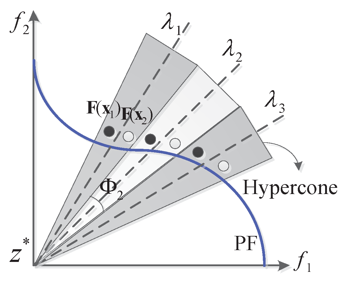
To enhance the convergence speed of the PBI method, while handling non-convex PF shapes in the meantime, a localized PBI (LPBI) is proposed [25]. In the LPBI method, the newly generated solution is merely compared with solutions that are inside the same hypercone, as shown in Figure 4, instead of the entire population.
Given N direction vectors, the objective space can be divided into N sub-regions (i.e., hypercone) by the LPBI method. In any hypercone, e.g., the i-th hypercone, the center line is assumed to be the associated direction vector . Correspondingly, the apex is obtained by averaging those angles between the and its m closest direction vectors (where m is the number of objectives, see Equation (16)):
where is the angle between the k-th closest direction vector and . For two vectors, e.g., and , the cosine value of the intersection angle is available by Equation (17):
For each , only solutions whose objective vectors are inside the associated hypercone are chosen. Taking Figure 4 as an example, the solution for is merely selected from and . Even though the value is small, e.g., , the objective vectors of the obtained solutions are still not quite far away from their reference direction lines () (see the solid dots (•)). To be exact, the angles formed by those objective vectors and their corresponding direction lines are no more than even in the worst case.
Overall, the LPBI method is responsible for obtaining an optimal solution within each hypercone. Ideally, the LPBI will find different optimal solutions along different direction vectors, providing a set of diversified solutions regardless of the PF shapes. Specifically, the LPBI is implemented as follows: the scalar values of solutions inside the hypercone are calculated by Equation (15), while those outside the hypercone are set to .
3.2. MOEA/D-LPBI
In this subsection, we incorporate the LPBI method into the MOEA/D framework. The pseudo code of the derived algorithm, denoted as MOEA/D-LPBI, is shown in Algorithm 2. Initially, a population of N individuals (solutions) is randomly generated, where is the -th individual. Also a set of evenly distributed direction vectors is generated, denoted as . Each individual, e.g., , is randomly paired-up with a direction vector, e.g., . For each direction vector, its neighbours (measured by the Euclidean distance) are found denoted as where is a user-defined positive integer. Their associated neighbouring solutions are denoted as . Then, the apex of the hypercone for each direction vector is computed by Equation (16).
| Algorithm 2: MOEA/D-LPBI. |
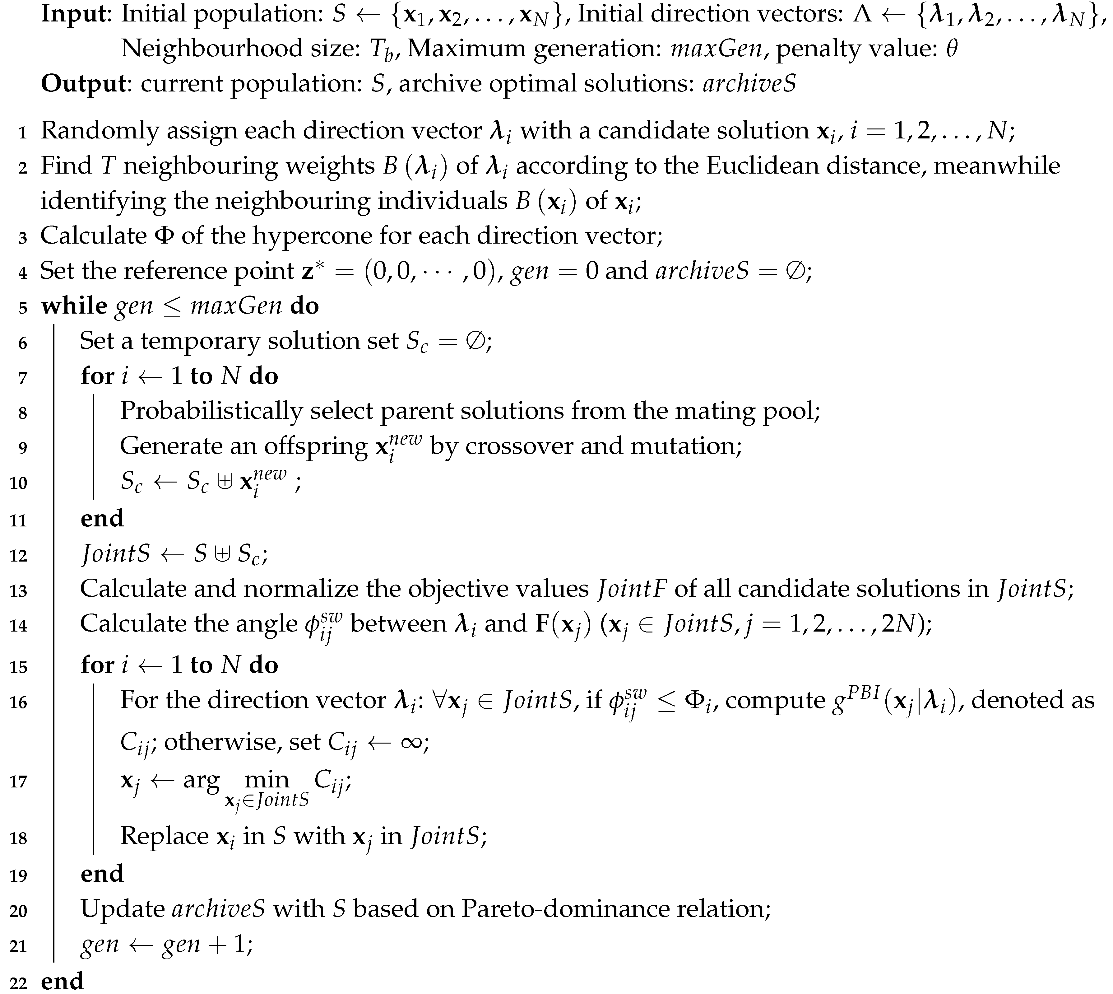 |
Following that, the population evolves for generations (lines 5 to 22). In lines 7–11, the parent set Q of is probabilistically selected from the neighbours or the whole population S, and is used to generate an offspring by the differential evolution (DE) and polynomial mutation (PM) operators [26]. Lines 12–14 merge the current population and the newly generated individuals, denoted as , and obtain the angle matrix . Note that the proposed algorithm is implemented within a () elitism framework [27]. For each vector, lines 15–19 select the solution whose PBI scalar values is the smallest amongst the according to the framework. At the end of each generation, the offline archive is updated with the newly obtained solutions based on the Pareto-dominance relation (line 20).
In terms of the time complexity of the derived algorithm (MOEA/D-LPBI), calculation of the scalar values of all individuals on all direction vectors runs at where N is the population size. Additionally, identifying the minimal PBI values from values runs at . Therefore, the overall time complexity of MOEA/D-LPBI is . In comparison, if the conventional method is adopted instead, all of the possible values of the variables need to be tried. Assuming that the precision accuracy is 0.01, the total complexity is which is far larger than that of MOEA/D-LPBI ( is a variable in the PV model).
4. Experimental Results
MOEA/D-LPBI is applied to solve the multi-objective HRES model after it has been examined on a set of MOP benchmarks (see Appendix A).
Prior to the optimization, the required parameter settings in the above equations are provided in Table 1 and Table 2. Among them, Table 1 shows the initial investment cost and the annual repair expenses of all the devices. In addition, the expenditure in replacing old batteries is similar to the initial cost, that is, equals . All of the other parameters of HRES are summarized in Table 2. Readers can refer to [17] for more details.
In addition, the data of the solar radiation intensity, the wind velocity and the environmental temperature over a year is considered as input data. They are assumed to be constants for every hour time step. Their distributions during a year as well as the annual load are shown in Figure 5. In this experiment, T is the total number of hours in a year (also the maximum simulation time) and is calculated as .
To obtain the best configuration of the HRES in the two modes, MOEA/D-LPBI is applied to handle the model. In addition, not only does the original MOEA/D-PBI serve as a reference, but also two classic algorithms, i.e., preference-inspired coevolutionary algorithms using goal vectors (PICEA-g) [17,28] and MOEA/D with the weighted Tchebycheff (MOEA/D-TE) [24], are compared with the proposed algorithm afterwards.
Related parameter settings of these algorithms are described below:
- Algorithm runs: the maximum generation is set to 50.
- Individuals: the population size is N = 100. Each candidate solution consists of six variables in the form: [], which, respectively, represent the number of four main components, the height of the wind tower and the inclination angle of the tilted PV panel. Assuming that each PV string connects four units in series, the number of is a multiple of four.
- MOEA/D parameters: the neighbourhood size is set to be 10 and the probability of selecting in the neighbourhood is set as . In the reference algorithm, the replacement size is 2.
- Penalty values: the considered penalty values are .
Simulations of the HRES in two modes are respectively operated. Note that the electricity price during peak period (8:00 to 22:00) and trough period (22:00 to 8:00 on the next day) in mode II is 0.2$/kWh and 0.1$/kWh, respectively. The MOEA/D-LPBI under various penalty values and its competitors are applied to obtain a set of Pareto optimal HRES configurations. To quantitatively compare these algorithms, the hypervolume (HV) is adopted to evaluate their performance. This indicator is one of the most frequently used performance metrics in literature [29], the larger value indicating the better performance. It is calculated as follows: first, all the objective values of solutions are normalized within [0,1], and then the HV metric measures the region enclosed by the normalized non-dominated solutions and a reference point , which is set to [1.1, 1.1,…, 1.1]. The mean HV results of the obtained solutions from 31 runs are shown in Table 3.
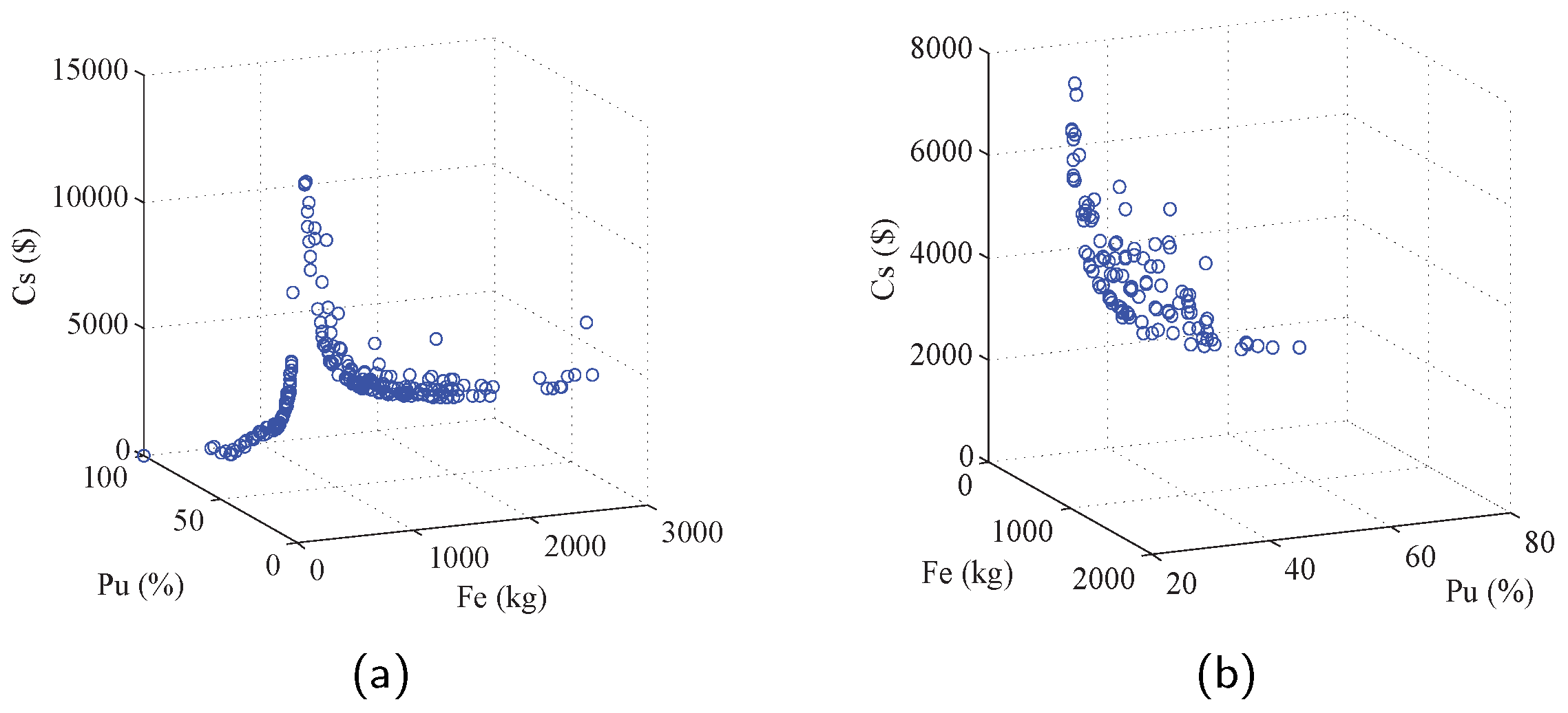
The results from Table 3 reveal that MOEA/D-LPBI obtains more competitive performances than the traditional framework for almost all penalty values. Moreover, MOEA/D-LPBI with performs best in both modes. The corresponding Pareto optimal solutions are plotted in Figure 6.
Provided the suitable penalty setting (i.e., ), the MOEA/D-LPBI is further compared with another two competitors. Similarly, their mean HV values are illustrated in Table 4 with the Wilcoxon-ranksum two-sided comparison [30] procedure at 95% confidence level employed.
Through quantitative comparison, the proposed algorithm (with ) is also shown to be superior than the classic versions PICEA-g and MOEA/D-TE.
Amongst the obtained Pareto optimal solutions by the MOEA/D-LPBI, a decision maker can choose the preferred one. For example,
- in mode I, if the decision maker prefers to meet the energy demand 100% and limit the emission within 250 kg, then one can set = 0% and . Then, the three filtered are shown in Table 5. Amongst these solutions, the one that produces the minimum cost is selected, i.e., the third one (in bold).
- in mode II, if the decision maker prefers to minimize the fuel emission and the utility of non-renewable energy, the solution having minimum and is selected, i.e., the first one (in bold). Additionally, it can be observed that the diesel generators are not used in this case.
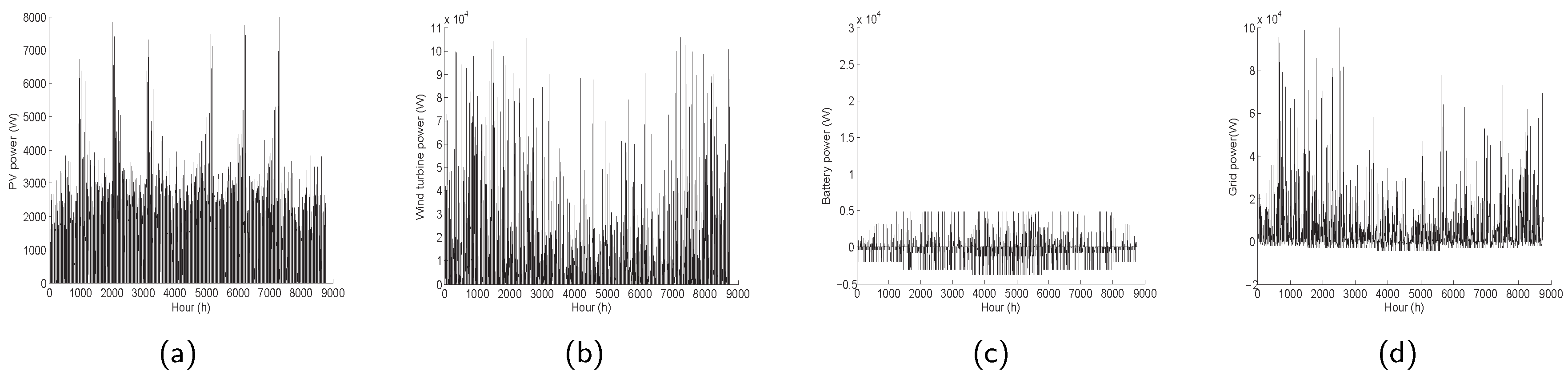
According to the selected results, the final optimal configurations of the HRESs in the two modes are confirmed. Their processes of supplying power during a year are simulated as shown in Figure 7 and Figure 8. It can be observed that the configuration is different in the two modes and the power grid takes the place of the diesel generators in mode II.
5. Conclusions
This paper studies the multi-objective optimal design of hybrid PV-wind-diesel-battery system for the power-supply, considering that three objectives are simultaneously to be minimized in the specialized operational mode. In mode I (isolated), the system relies on the battery storage and the diesel generator to supplement deficit power; in mode II (grid-connected), it prefers buying power from the power grid to using the diesel generators (under the provided parameters). By a MOEA/D using localized PBI, denoted as MOEA/D-LPBI, a set of Pareto optimal configurations of the HRES in each mode is obtained, from which a decision maker can choose the most adequate one. In addition, experimental results have also demonstrated that the MOEA/D-LPBI outperforms its competitor MOEA/D-PBI for MOPs with different PF shapes.
In terms of future studies, the first optimal design of HRES in view of many-objective optimization [26,28] and/or interactive decision making [31] will be investigated. Second, regarding the algorithm design, we would like to examine the effect of reference point in decomposition based algorithms [32], and the performance of LPBI on convex PFs.
Supplementary Materials
Source code of MOEA/D-LPBI is available online at http://ruiwangnudt.gotoip3.com/optimization.html.
Acknowledgments
This work is supported by the National Natural Science Foundation of China (Nos. 61403404 and 71571187) and the Outstanding Natural Science Foundation of Hunan Province (2017JJ1001).
Author Contributions
Mengjun Ming and Rui Wang designed and realized the algorithm; Tao Zhang conceived the control strategy of the system; Yabing Zha contributed to the application and provided helpful advice; and Mengjun Ming and Rui Wang wrote the paper.
Conflicts of Interest
The authors declare no conflict of interest.
Appendix A
The test problems are constructed by performing different shape constrains in the Walking Fish Group (WFG) kit to the standard WFG4 benchmark problem [20,21]. Taking WFG45 as an example, its PF is mixed, combining the concave and the convex.
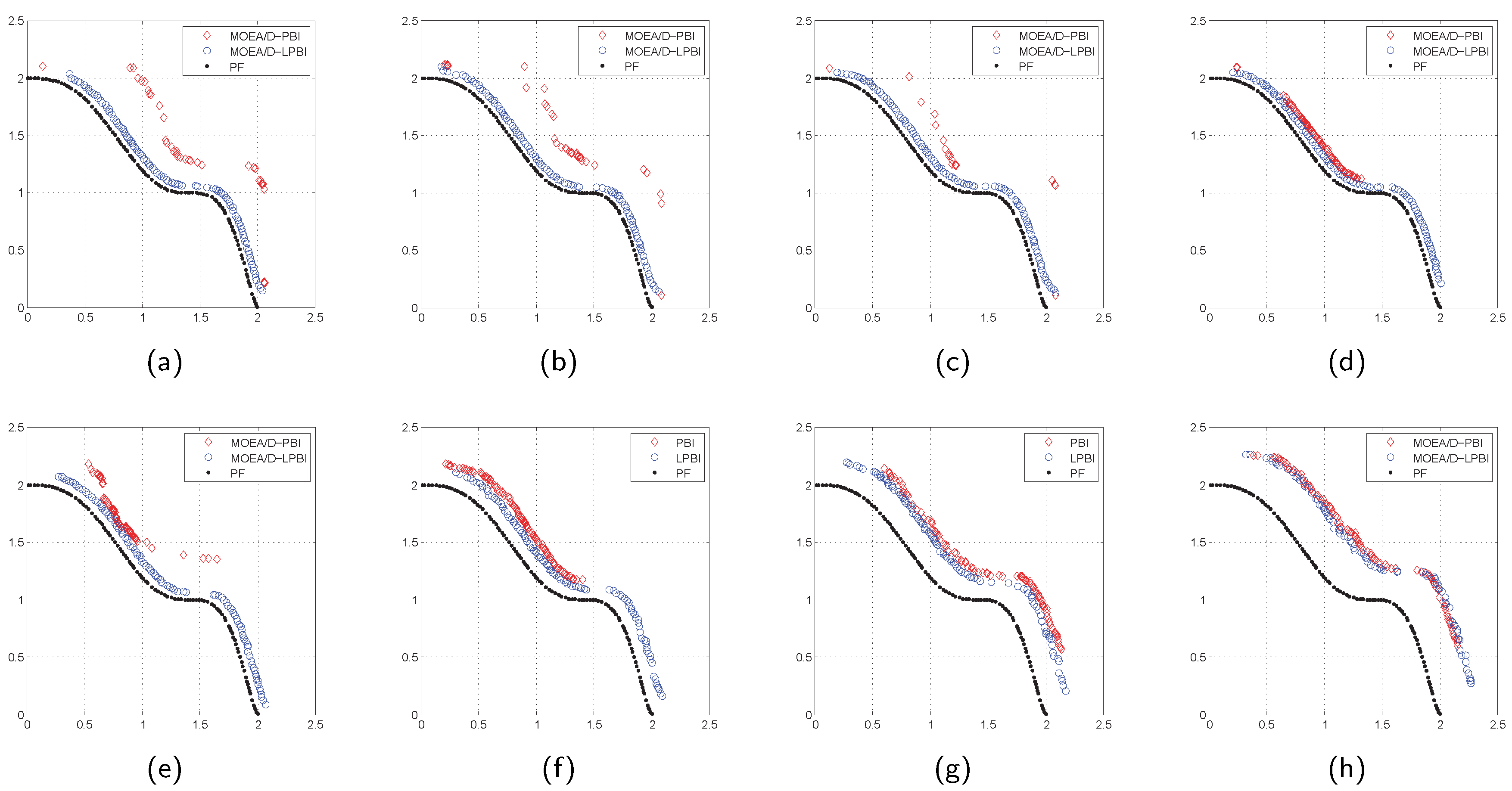
MOEA/D-LPBI and its competitor MOEA/D-PBI are generally performed for 31 runs under the considered penalty value set (). Figure A1 shows the obtained non-dominated solutions for the bi-objective WFG45 problem, allowing visual inspection of their proximity and diversity. The true PF serves as the reference.
Figure A1.
The approximation of Pareto front (PF) under different penalty values for Walking Fish Group (WFG)45-2 (color online). (a) ; (b) ; (c) ; (d) ; (e) ; (f) ; (g) ; and (h) .
Figure A1.
The approximation of Pareto front (PF) under different penalty values for Walking Fish Group (WFG)45-2 (color online). (a) ; (b) ; (c) ; (d) ; (e) ; (f) ; (g) ; and (h) .

Figure A1 demonstrates that MOEA/D-LPBI exhibits excellent performance and is robust to the PFs, that is, the solutions nearly cover the whole PF region and are close to the PF regardless of the choice of . However, the performance of MOEA/D-PBI varies significantly and is inferior to the improved version for all problems.
Though only the comparison results for WFG45-2 are shown, similar results are obtained for other problems (see our previous work [25]).
References
- Zeng, J.; Li, M.; Liu, J.F.; Wu, J.; Ngan, H.W. Operational optimization of a stand-alone hybrid renewable energy generation system based on an improved genetic algorithm. In Proceedings of the 2010 IEEE Power and Energy Society General Meeting, Providence, RI, USA, 25–29 July 2010. [Google Scholar]
- Niknam, T.; Taheri, S.I.; Aghaei, J.; Tabatabaei, S.; Nayeripour, M. A modified honey bee mating optimization algorithm for multiobjective placement of renewable energy resources. Appl. Energy 2011, 88, 4817–4830. [Google Scholar] [CrossRef]
- Wang, R.; Fleming, P.J.; Purshouse, R.C. General framework for localised multi-objective evolutionary algorithms. Inf. Sci. 2014, 258, 29–53. [Google Scholar] [CrossRef]
- Fadaee, M.; Radzi, M.A.M. Multi-objective optimization of a stand-alone hybrid renewable energy system by using evolutionary algorithms: A review. Renew. Sustain. Energy Rev. 2012, 16, 3364–3369. [Google Scholar] [CrossRef]
- Dufo-López, R.; Bernal-Agustín, J.L. Design and control strategies of PV-Diesel systems using genetic algorithms. Sol. Energy 2005, 79, 33–46. [Google Scholar] [CrossRef]
- Dufo-López, R.; Contreras, J. Optimization of control strategies for stand-alone renewable energy systems with hydrogen storage. Renew. Energy 2007, 32, 1102–1126. [Google Scholar] [CrossRef]
- Dufo-López, R.; Bernal-Agustín, J.L. Multi-objective design of PV-wind-diesel–hydrogen–battery systems. Renew. Energy 2008, 33, 2559–2572. [Google Scholar] [CrossRef]
- Trivedi, M. Multi-Objective Generation Scheduling with Hybrid Energy Resources. Ph.D. Thesis, Department of Electrical Engineering, Clemson University, Clemson, SC, USA, 2007. [Google Scholar]
- Masoum, M.A.S.; Badejani, S.M.M.; Kalantar, M. Optimal placement of hybrid PV-wind systems using genetic algorithm. In Proceedings of the Innovative Smart Grid Technologies, Gaithersburg, MD, USA, 19–21 January 2010; pp. 1–5. [Google Scholar]
- Katsigiannis, Y.A.; Georgilakis, P.S.; Karapidakis, E.S. Multiobjective genetic algorithm solution to the optimum economic and environmental performance problem of small autonomous hybrid power systems with renewables. IET Renew. Power Gener. 2010, 4, 404–419. [Google Scholar] [CrossRef]
- Srinivas, N.; Deb, K. Muiltiobjective Optimization Using Nondominated Sorting in Genetic Algorithms. Evolut. Comput. 2007, 2, 221–248. [Google Scholar] [CrossRef]
- Zhang, Q.; Li, H. MOEA/D: A Multiobjective Evolutionary Algorithm Based on Decomposition. IEEE Trans. Evolut. Comput. 2007, 11, 712–731. [Google Scholar] [CrossRef]
- Wang, R.; Zhang, F.; Zhang, T. Multi-objective optimal design of hybrid renewable energy systems using evolutionary algorithms. In Proceedings of the 2015 11th International Conference on Natural Computation (ICNC), Zhangjiajie, China, 15–17 August 2015; pp. 1196–1200. [Google Scholar]
- Myrzik, J.M.A.; Calais, M. String and module integrated inverters for single-phase grid connected photovoltaic systems—A review. In Proceedings of the 2003 IEEE Bologna Power Tech Conference Proceedings, Bologna, Italy, 23–26 June 2003; Volume 2, p. 8. [Google Scholar]
- Fei, W. Research on Photovoltaic Grid-Connected Power System. Trans. China Electrotech. Soc. 2005, 20, 72–74, 91. [Google Scholar]
- Koutroulis, E.; Kolokotsa, D.; Potirakis, A.; Kalaitzakis, K. Methodology for optimal sizing of stand-alone photovoltaic/wind-generator systems using genetic algorithms. Sol. Energy 2006, 80, 1072–1088. [Google Scholar] [CrossRef]
- Shi, Z.; Wang, R.; Zhang, T. Multi-objective optimal design of hybrid renewable energy systems using preference-inspired coevolutionary approach. Sol. Energy 2015, 118, 96–106. [Google Scholar] [CrossRef]
- Yang, H.; Lu, L.; Zhou, W. A novel optimization sizing model for hybrid solar-wind power generation system. Sol. Energy 2007, 81, 76–84. [Google Scholar] [CrossRef]
- Yang, H.; Zhou, W.; Lu, L.; Fang, Z. Optimal sizing method for stand-alone hybrid solar–wind system with LPSP technology by using genetic algorithm. Sol. Energy 2008, 82, 354–367. [Google Scholar] [CrossRef]
- Wang, R.; Purshouse, R.C.; Fleming, P.J. Preference-inspired co-evolutionary algorithms using weight vectors. Eur. J. Oper. Res. 2015, 243, 423–441. [Google Scholar] [CrossRef]
- Wang, R.; Zhang, Q.; Zhang, T. Decomposition based algorithms using Pareto adaptive scalarizing methods. IEEE Trans. Evolut. Comput. 2016, 20, 821–837. [Google Scholar] [CrossRef]
- Li, K.; Kwong, S.; Zhang, Q.; Deb, K. Interrelationship-Based Selection for Decomposition Multiobjective Optimization. IEEE Trans. Cybern. 2015, 45, 2076–2088. [Google Scholar] [CrossRef] [PubMed]
- Mohammadi, A.; Omidvar, M.N.; Li, X.; Deb, K. Sensitivity analysis of Penalty-based Boundary Intersection on aggregation-based EMO algorithms. In Proceedings of the 2015 IEEE Congress on Evolutionary Computation, Sendai, Japan, 25–28 May 2015. [Google Scholar]
- Ishibuchi, H.; Akedo, N.; Nojima, Y. A study on the specification of a scalarizing function in MOEA/D for many-objective knapsack problems. In Learning and Intelligent Optimization; Springer: Berlin, Germany, 2013; pp. 231–246. [Google Scholar]
- Wang, R.; Ishibuchi, H.; Zhang, Y.; Zheng, X.; Zhang, T. On the effect of localized PBI method in MOEAD for multi-objective optimization. In Proceedings of the 2016 IEEE Symposium Series on Computational Intelligence, Athens, Greece, 6–9 December 2016; pp. 647–650. [Google Scholar]
- Wang, R.; Zhou, Z.; Liao, T.; Zhang, T. Localized weighted sum method for many-objective optimization. IEEE Trans. Evolut. Comput. 2016, PP, 1. [Google Scholar] [CrossRef]
- Deb, K.; Pratap, A.; Agarwal, S.; Meyarivan, T. A fast and elitist multiobjective genetic algorithm: NSGA-II. IEEE Trans. Evolut. Comput. 2002, 6, 182–197. [Google Scholar] [CrossRef]
- Wang, R.; Purshouse, R.C.; Fleming, P.J. Preference-inspired Co-evolutionary Algorithms for Many-objective Optimisation. IEEE Trans. Evolut. Comput. 2013, 17, 474–494. [Google Scholar] [CrossRef]
- Zitzler, E.; Thiele, L.; Laumanns, M.; Fonseca, C.M.; Fonseca, V.G.D. Performance assessment of multiobjective optimizers: An analysis and review. IEEE Trans. Evolut. Comput. 2003, 7, 117–132. [Google Scholar] [CrossRef]
- Hollander, M.; Wolfe, D. Nonparametric Statistical Methods; Wiley-Interscience: Boston, MA, USA, 1999. [Google Scholar]
- Wang, R.; Purshouse, R.C.; Giagkiozis, I.; Fleming, P.J. The iPICEA-g: A new hybrid evolutionary multi-criteria decision making approach using the brushing technique. Eur. J. Oper. Res. 2015, 243, 442–453. [Google Scholar] [CrossRef]
- Wang, R.; Xiong, J.; Ishibuchi, H.; Wu, G.; Zhang, T. On the effect of reference point in MOEA/D for multi-objective optimization. Appl. Soft Comput. 2016, 58, 25–34. [Google Scholar] [CrossRef]
Figure 1.
Illustration of the hybrid renewable energy system (HRES) with power grid. PV: photovoltaic.
Figure 1.
Illustration of the hybrid renewable energy system (HRES) with power grid. PV: photovoltaic.

Figure 2.
Illustration of the energy flow in the HRES.
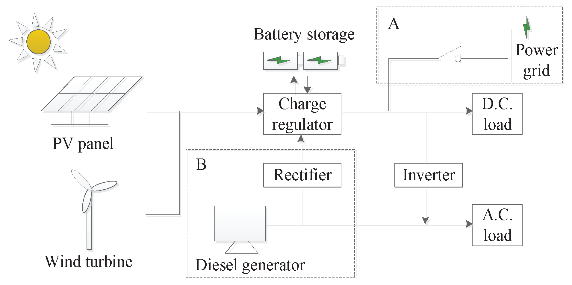
Figure 3.
Flowchart of system simulation. (a) the isolated-island mode; and (b) the grid-connected mode. SOC: state of charge.
Figure 3.
Flowchart of system simulation. (a) the isolated-island mode; and (b) the grid-connected mode. SOC: state of charge.

Figure 4.
Demonstration of the localized localized penalty-based boundary intersection (LPBI) method.
Figure 4.
Demonstration of the localized localized penalty-based boundary intersection (LPBI) method.

Figure 5.
Hourly mean values of meteorological conditions. (a) solar irradiation; (b) wind velocity; (c) temperature; and (d) load.
Figure 5.
Hourly mean values of meteorological conditions. (a) solar irradiation; (b) wind velocity; (c) temperature; and (d) load.
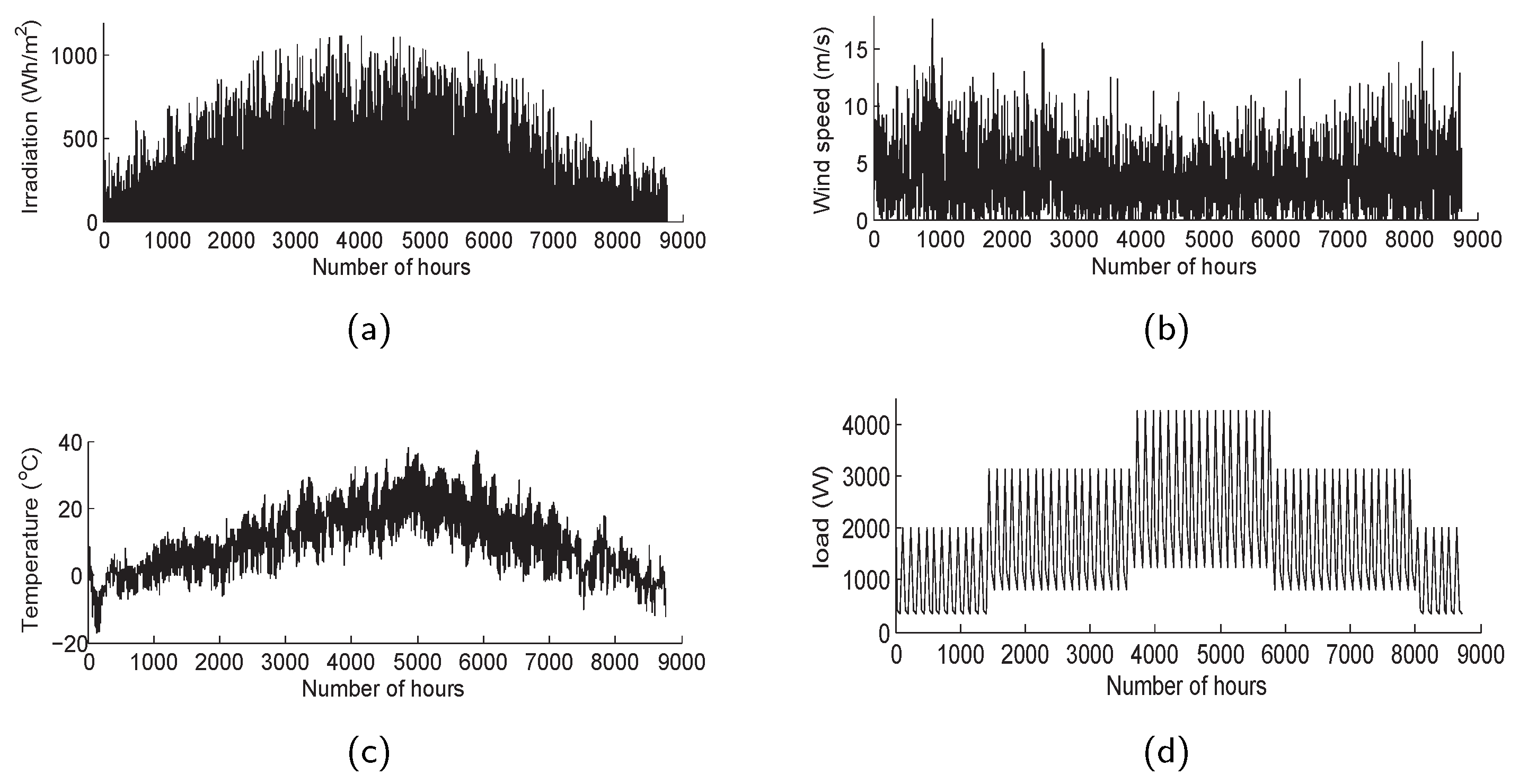
Figure 6.
Optimal solutions for HRES in different modes. (a) mode I; and (b) mode II.

Figure 7.
Power generation in mode I. (a) PV; (b) wind generator; (c) battery; (d) diesel generator.
Figure 7.
Power generation in mode I. (a) PV; (b) wind generator; (c) battery; (d) diesel generator.
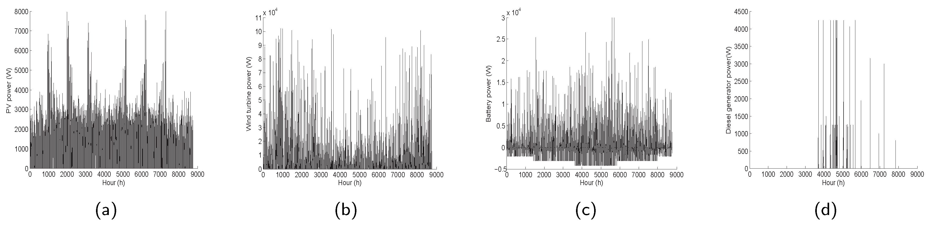
Figure 8.
Power generation in mode II. (a) PV; (b) wind generator; (c) battery; and (d) power grid.


Table 1.
The initial cost (per unit) and the annual repair expenses of the system components in HRES.
Table 1.
The initial cost (per unit) and the annual repair expenses of the system components in HRES.
| Cost | PV Panel | Wind Turbine | Wind Tower | Battery | Diesel Generator | Inverter | Rectifier |
|---|---|---|---|---|---|---|---|
| ($) | 300 | 3000 | 250/m | 126 | 1514 | 240 | 225 |
| ($) | 30 | 50 | 2.5/m | 1.26 | 0.17/h | 12 | 8 |
Table 2.
Parameter specifications for the environment and the system components.
| Parameter | Value | Parameter | Value | Parameter | Value |
|---|---|---|---|---|---|
| 0.73 | 12.59 | 1 | |||
| (m/s) | 4 | (kW) | 1 | (kW) | 2 |
| (m/s) | 14 | 10 | (L/kWh) | 0.08 | |
| (m/s) | 20 | (Ah) | 100 | (L/kWh) | 0.25 |
| 0.4 | (V) | 12 | (kg/L) | 2.5 | |
| (kg/) | 1.29 | 0.2 | ($/L) | 1.2 |
Table 3.
The mean hypervolume (HV) results of MOEA/D-LPBI and the original version with different for HRES. The symbol “+”, “−” or “=” means that the counterpart is statistically better than, worse than or comparable to MOEA/D-LPBI. The best HV value for each problem is marked in boldface.
Table 3.
The mean hypervolume (HV) results of MOEA/D-LPBI and the original version with different for HRES. The symbol “+”, “−” or “=” means that the counterpart is statistically better than, worse than or comparable to MOEA/D-LPBI. The best HV value for each problem is marked in boldface.
| HRES | Algorithm | ||||||||
|---|---|---|---|---|---|---|---|---|---|
| mode I | PBI | 0.921 | 0.903 | 0.907 | 0.710 | 0.569 | 0.694 | 0.723 | 0.704 |
| LPBI | 0.947 | 0.865 | 0.923 | 0.948 | 0.957 | 0.891 | 0.965 | 0.963 | |
| mode II | PBI | 0.622 | 0.621 | 0.646 | 0.616 | 0.620 | 0.559 | 0.632 | 0.585 |
| LPBI | 0.625 | 0.647 | 0.658 | 0.695 | 0.700 | 0.662 | 0.710 | 0.702 |
Table 4.
The mean HV results and the standard deviations (in the parentheses) of MOEA/D-LPBI, PICEA-g and MOEA/D-TE for HRES. Just as above, their comparable results are marked by “+”, “−” or “=”.
Table 4.
The mean HV results and the standard deviations (in the parentheses) of MOEA/D-LPBI, PICEA-g and MOEA/D-TE for HRES. Just as above, their comparable results are marked by “+”, “−” or “=”.
| HV | MOEA/D-LPBI | PICEA-g | MOEA/D-TE |
|---|---|---|---|
| mode I | 0.965 (0.089) | 0.892 (0.112) | 0.935 (0.127) |
| mode II | 0.710 (0.068) | 0.655 (0.077) | 0.681 (0.043) |
Table 5.
Selected results using MOEA/D-LPBI with specified reference.
| Mode I | |||||||||
| Solution | (kg) | ($) | |||||||
| 1 | 28 | 17 | 30 | 5 | 21.605 | 58.545 | 109.404 | 0 | 13,324.550 |
| 2 | 28 | 18 | 30 | 8 | 14.546 | 59.662 | 151.846 | 0 | 12,345.850 |
| 3 | 28 | 12 | 28 | 7 | 19.081 | 48.441 | 219.842 | 0 | 10,186.780 |
| Mode II | |||||||||
| Solution | (kg) | ($) | |||||||
| 1 | 28 | 12 | 4 | 0 | 30 | 46.733 | 0 | 34.085 | 5733.406 |
| 2 | 28 | 11 | 4 | 0 | 30 | 49.870 | 0 | 34.243 | 5416.173 |
| 3 | 28 | 7 | 3 | 0 | 26.597 | 46.099 | 0 | 36.245 | 3903.858 |
© 2017 by the authors. Licensee MDPI, Basel, Switzerland. This article is an open access article distributed under the terms and conditions of the Creative Commons Attribution (CC BY) license (http://creativecommons.org/licenses/by/4.0/).
Share and Cite
MDPI and ACS Style
Ming, M.; Wang, R.; Zha, Y.; Zhang, T. Multi-Objective Optimization of Hybrid Renewable Energy System Using an Enhanced Multi-Objective Evolutionary Algorithm. Energies 2017, 10, 674. https://doi.org/10.3390/en10050674
AMA Style
Ming M, Wang R, Zha Y, Zhang T. Multi-Objective Optimization of Hybrid Renewable Energy System Using an Enhanced Multi-Objective Evolutionary Algorithm. Energies. 2017; 10(5):674. https://doi.org/10.3390/en10050674
Chicago/Turabian StyleMing, Mengjun, Rui Wang, Yabing Zha, and Tao Zhang. 2017. "Multi-Objective Optimization of Hybrid Renewable Energy System Using an Enhanced Multi-Objective Evolutionary Algorithm" Energies 10, no. 5: 674. https://doi.org/10.3390/en10050674
Note that from the first issue of 2016, this journal uses article numbers instead of page numbers. See further details here.