1. Introduction
The distribution generation (DG) integration in distribution networks (DNs) has become a hot research topic. By allocating DG units at appropriate positions, load balancing and line loss minimization may be achieved after power flow optimization. In the meanwhile, DN structures may make necessary adjustments. After establishing a feasible radial distribution structure, DG units can be set with adjusted output in the reconfigured network to further improve the optimization results.
Network reconfiguration is the process of altering the open/closed status of sectionalizing and loop switches, thus adapting a new topological structure for reducing power losses and improving system reliabilities. The network reconfiguration process is often investigated under two circumstances: (1) reconfiguration for power service restoration; (2) scheduled reconfiguration due to seasonal variation and larger load changes. The former process is a nearly real-time optimization, while the latter can and should be planned before application. The essential motivation for reconfiguration is to reduce economic losses, which will take switch operation and mean time to restoration into consideration. From the perspective of distribution system operation, uncertainties are inevitable due to the sequential effects and environmental factors present in a DN. These uncertainties may be embodied as variability and incertitude in equipment and electrical parameters, such as fault rate of generators and load fluctuations.
As a non-differentiable constrained and non-linear programming problem, many algorithms have been proposed to solve the network reconfiguration issue. References [
1,
2,
3,
4,
5] investigated how heuristic algorithms were applied in finding optimal network structures. Dai and Sheng [
1] studied the network reconfiguration problem by combining a two-stage optimization problem, and only load data uncertainty was considered. Gomes and Carneiro [
2] studied an improved heuristic algorithm to find optimal network structures. They took all weak loops into consideration at once and established a maneuvering list, then tried to open each weak loop according to the list, till the network became radial again. Gonzalez et al. [
3] determined switch status by sensitivity analysis, thus avoiding repeated calculations. Zhang and Li [
4] utilized the topology characteristic of networks to propose a heuristic method to determine the optimal solution after a short iteration. Rugthaicharoenchep et al. [
5] applied a greedy algorithm to solve the multi-objective reconfiguration problem for power loss reduction and load balancing.
A considerable number of intelligent algorithms are also applied to reconfiguration problems. References [
6,
7,
8] proposed three different methods derived from a genetic algorithm (GA) respectively. Prasad et al. [
6] improved random evolution rules, making it possible to deal with discrete variables, and avoided islands and loops by improving encoding. Mendoza et al. [
7] proposed accentuated crossover and directed mutation, reducing searching space and memory occupation. Enacheanu et al. [
8] combined GA with graph theories to select an efficient mutation, making all the resulting individuals feasible.
As for other intelligent algorithms, Chang [
9] proposed an application for the ant colony search algorithm in reconfiguration and capacitor placement. The algorithm kept the mutation towards optimization by setting pheromone-updating rules. Liu and Gu [
10] proposed an improved discrete particle swarm optimization (PSO), in which they defined an efficiency index to evaluate feasible structures before applying the algorithm. Wu et al. [
11] improved the integer coded PSO method by adding historically optimal solutions to new particle creation, directing the search to optimization.
To deal with uncertainties in DN systems, different methods had been investigated. Load uncertainty had been investigated in the recent literature. Lee et al. [
12] proposed a two-stage robust optimization model for the distribution network reconfiguration problem with load uncertainty. Bai et al. [
13] analyzed measured network data taking into account the issue of substation time-varying loads and uncertainty. Zhang and Li [
4] utilized interval analysis in a heuristic method to demonstrate how uncertain parameters influenced the reconfiguration result. They chose reliabilities and economy as the main objectives instead of solely power loss optimization. Muñoz et al. [
14] applied affine arithmetic method to a voltage stability assessment, and reduced the computation burden as compared to Monte Carlo simulations. Vaccaro et al. [
15] presented a range arithmetic method for power flow problems including interval data. Rakpenthai et al. [
16] utilized synchronized phasor measurement data and state variables expressed in rectangular forms to formulate the state estimation under the transmission line parameter uncertainties based on the weight least square criterion as a parametric interval linear system of equations.
DG units can be involved in the network operation as ancillary services [
17,
18]. To integrate DG in DN, the location and regulation for DG units are the main optimization problems in network reconfiguration [
19,
20,
21,
22]. Some representative methods were proposed in recent references. Pavani and Singh [
23] allocated DG units on specific buses after the network had been optimized by a heuristic method, reducing the power loss on feeders. Rao et al. [
24] applied a Harmony Search Algorithm (HSA) in DG setting combined with reconfiguration, and proved the method was effective under different load levels.
Although the attention of the previous works has been focused on those points mentioned separately, relatively little effort was directed to considering reconfiguration, reliability evaluation, interval analysis and DG allocation simultaneously. In this paper, the multi-objective network reconfiguration optimization model is formulated with the consideration of minimum line loss, minimum Expected Energy Not Supplied (EENS) and minimum switch operation cost, and then the optimization problem is solved by combining Binary Particle Swarm Optimization (BPSO) and HSA considering the DG placement. Further, interval analysis is applied to deal with equipment parameters and load data uncertainties.
The remainder of this paper is organized as follows:
Section 2 formulates the proposed multi-objective optimization problem for network reconfiguration. The proposed method to solve the optimization problem is described in
Section 3.
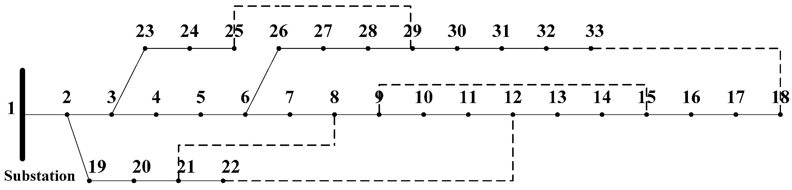
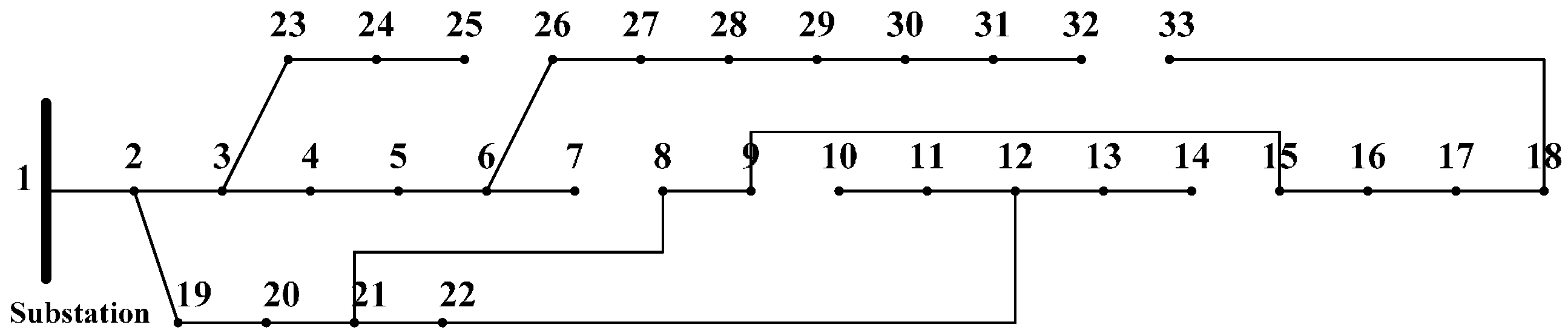
Section 4 provides numerical results and comparisons of the proposed approach using multiple test systems with DG units.
Section 5 summarizes the main contributions and conclusions of this paper.
3. The Proposed DN Reconfiguration Algorithm
3.1. Overview
Network reconfiguration with the consideration of DG placement is a combination of discrete and continuous problems. In this paper, a method is proposed to process the discrete and continuous variables, and then the problem is optimized comprehensively. To generate a feasible network topology, BPSO is applied to solve a multi-objective optimization of line loss and system reliability. Based on the given network, DG unit locations are chosen by sensitivity analysis. Further the sizing problem of DG units is optimized in HSA. HSA is a meta-heuristic algorithm inspired by the improvisation process of a musician. In HSA, each musician which represents a decision variable, plays a note, namely generates a value, to obtain a best harmony which represents the global optimum. HSA does not require initial values for the decision variables, and it has less parameters and is easy to implement. It has been successfully applied to various power system research problems.
3.2. Sensitivity Analysis with Loss Sensitivity Factors
Sensitivity analysis is often utilized in DG placement [
28]. The candidate locations for DG units are determined by calculating the sensitivity factors of buses in the network. This process will help narrow the search space for the optimization procedure.
The sensitivity factor can be defined as the derivation form of Equation (3). Since the factor is the derivative of power loss with respect to bus load, the factor is called Loss Sensitivity Factor (LSF), which can be expressed as:
Based on Equation (14), the LSFs of all buses can be calculated and arranged in descending order. The order determines the priority of buses to be considered as DG locations. After the candidate buses are chosen, the size of the DG can then be calculated using HSA.
3.3. DG Modeling
This paper is concerned with DG output planning and not real-time dispatching, which means a DG model which can be smoothly adjusted while keeping power factor stable is required. Based on this consideration, a wind turbine (WT) is chosen as a typical model.
Different types of WTs are applied under different circumstances including synchronous generator (SG) and asynchronous generator (AG). Among them, the Doubly Fed Induction Generator (DFIG) is chosen as the DG model in this paper. These generators can smoothly adjust their real power output, while keeping power factor stable with reactive power compensation equipment. Then the DG units can be modeled as negative PQ-type loads:
where
and
are the real and reactive power load at node
after the DG is placed.
and
are the real and reactive power output of DG units, respectively.
3.4. Generating Feasible Solution Algorithm Using BPSO
BPSO is a binary version of the PSO algorithm in which a velocity limitation would be needed to make sure solutions don’t fall into local optima. In this paper, BPSO is utilized to search for feasible network reconfiguration solutions. The sigmoid function is utilized to reflect the mapping relation between particle velocity and probability to be chosen, and ensures the result to be global optimal. The procedure of BPSO can be described as follows:
- Step (1)
Describe the status of all switches as array containing only 0 and 1, which means open and closed status respectively. Calculate objective function value for the initial system with , save the evaluation index.
- Step (2)
Generate the adjacent branch matrix and bus incidence matrix of the system. Search for loops formed by closing sectional switches, and save the loops as arrays .
- Step (3)
Generate the particle swarm: for every loop in
, after all the loops are opened, a new particle
is then formed. In BPSO, the location and velocity of particles are expressed as two vectors. Location represents the switch status and velocity influences the possibility for location to change, which can be expressed as:
where
is the dimension of particles.
To deal with opening loop process, the displacement formula of BPSO is as follows:
where
is threshold, typically set to 0.5 as default. The open switch is randomly selected among the zero elements of array
in each loop. After the selection, a new particle is formed. The loops in
may have overlay parts, so rules must be made to avoid them from choosing the same switch to open.
After a particle is formed, it needs to be checked by topology analysis to make sure that it represents a feasible solution.
- Step (4)
Repeat Step 3 until the swarm size meets the requirement.
- Step (5)
Generate solutions using BPSO and perform a topology analysis. Calculate the objective function value and save the evaluation index including power loss, reliabilities, total cost, etc. If the evaluation index of the solution is better than the historically best one, the index will be updated.
- Step (6)
Do Step 5 until the iteration reaches the maximal iteration , or the required accuracy is satisfied. Output the best index and the topology structure.
3.5. Topology Analysis
Topology analysis can detect whether the network generated by BPSO has loops or islands. Since the particle generating process determines that the network must be open loop, the system will not contain any closed loops. The topology analysis is applied to detect islands in the system.
As a network generated by BPSO, its bus incidence matrix is marked as
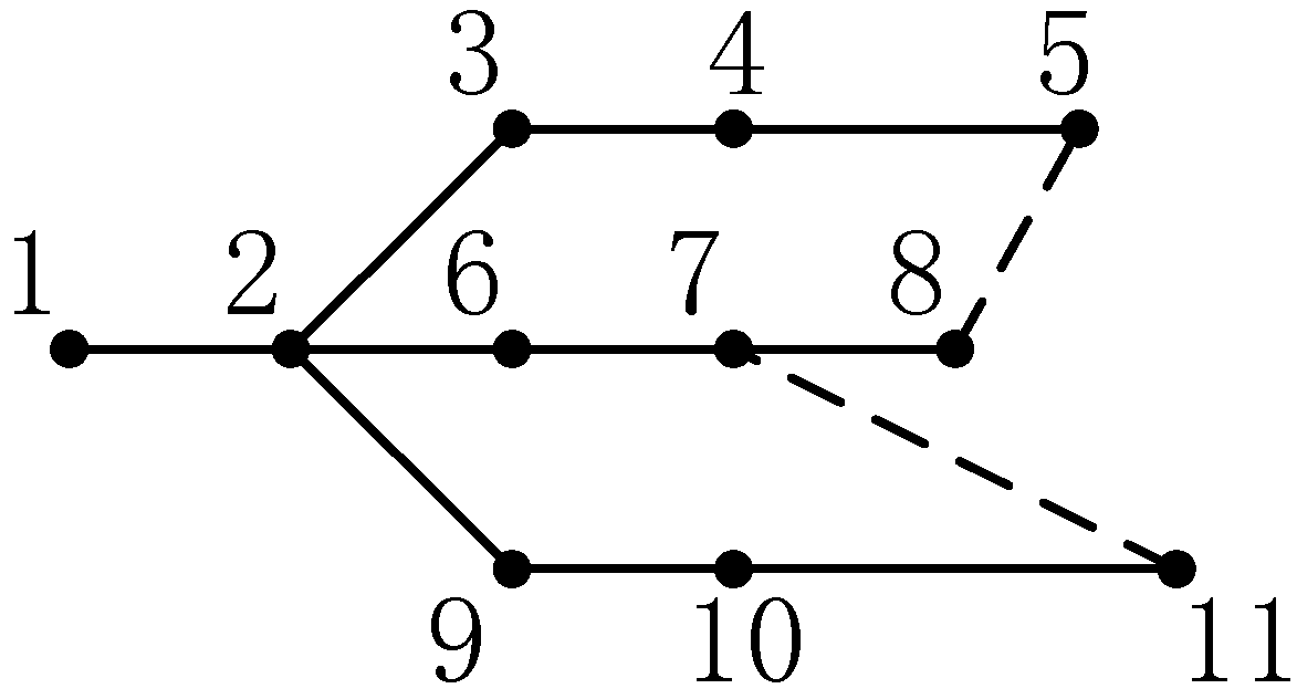
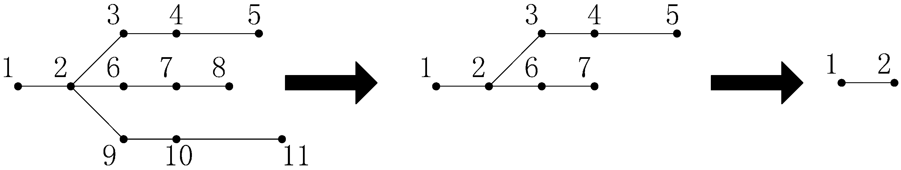
B. Each row shows the connection between one certain bus and all others, in which 1 means connected and 0 unconnected. The sum of each row is the grade of each node, which denotes the connection relation extent between this node and others. Apparently, the grade of an isolated bus is 0. The head or end node of the network is 1. The grade of other nodes is equal or greater than 2. The demonstration of topology analysis is based on the 11-bus system shown in
Figure 1. The node incidence matrix when the system is running in normal status is shown as:
The proposed method to find island system is as follows:
- Step (1)
Calculate grades of all the nodes in node incidence matrix B. Check if there is any node with grade 0. If the grade of any node is equal to 0, then it denotes that there is island node, which means the formed network structure is not feasible;
- Step (2)
If there is no island node, then delete the maximal node number with grade that equals to 1, namely deleting the corresponding row and column, and go to Step 1;
- Step (3)
Repeat step 1~2 until the network has only two nodes. If they aren’t nodes whose grade equals to 0, the network structure is proved to be feasible.
The process will reduce the rank of matrix B by 1 each time. For example, after utilizing the above method for 4 times, the matrix is shown as:
In the residual matrix, rows (or columns) representing grade-1 buses are 1, 5 and 7, namely the buses 1, 5 and 7 in the original system. Step 2 only reduces the system’s dimension, while keeping its topology structure. As the procedure continues, the matrix will finally become a 2-bus system, and the grades of remaining buses are both 1, which meets the termination condition of the operation. This proves that the original network structure doesn’t contain any islands. The process in topology structure is shown in
Figure 2.
3.6. Interval Analysis Method
To deal with uncertain factors in different mathematic models, interval analysis was proposed by Moore [
29]. The basic principles in interval calculation are as follows:
where
and
represent two sets. In Moore’s theory, the interval calculation can be done by using only their bounds, namely
. Based on this, the elementary operations are theoretically described in Equation (20). These operations represent add, subtract, multiply and divide in interval calculation respectively. In power systems interval analysis is usually applied in power flow calculations. The method varies in different algorithms. In recent research, some researchers proposed different methods to deal with interval data in power system. In this paper, interval analysis is applied into FBSM. There are two procedures in each iteration, which can be described as follows:
- (1)
Backward process: From the interval voltage vector of bus and interval current vector into bus k, calculate the interval voltage vector of bus and interval current vector out of bus .
- (2)
Forward process: From the interval voltage vector of bus and interval current vector out of bus , calculate the interval voltage vector of bus k and interval current vector into bus .
By applying the interval calculation principles in the Equations (1) and (2) mentioned in
Section 2, the interval form of FBSM is given as:
From the equations shown above, each variable appears only once in every FBSM iteration, thus keeping the interval calculation not so conservative. As for complexity, the interval FBSM costs only two times more than that the traditional FBSM, while the Newton method needs more memory space and calculation time to update the modified matrix. If the optimal solution is in interval form, then an intervals comparison is inevitable. For two intervals [A] and [B], it’s easy when [A] and [B] don’t share any common part. If they do have an overlapped area, then we pick two random variables from [A] and [B], respectively. Mark as event P, and assume values in the two intervals are uniformly distributed. The probability of P then can be calculated to evaluate the coverage of [A] on [B]. After this process, the result can be compared and optimization can be achieved.
3.7. Optimal DG Sizing Based on HSA
HSA can deal with continuous variables with the merit of many stochastic optimization methods [
30]. To optimize sizing after network reconfiguration, the process of applying HSA is as follows:
- Step (1)
Save the optimal network structure output by BPSO as array , and generate the HSA objective function with . Multiple DG capacities are set as independent variables.
- Step (2)
Generate initial harmony vectors. The parameters need to be given before initialization process are: Harmony Matrix (HM); Harmony Memory Size (HMS), Harmony Memory Considering Rate (HMCR), Pitch Adjusting Rate (PAR), and Number of Improvisations (NI).
- Step (3)
Improvise a new harmony vector.
In this step,
PAR is defined as a dynamic value, and a coefficient factor
is also defined as follows:
where
, and
are the ranges of
PAR;
is the current iteration number;
is the maximum number of iterations;
and
are the bounds of
.
is defined as:
With the improvement in (22) and (23), PAR and fw can adapt themselves to the optimization as the HSA iteration goes on: in the early iterations, new values within a wide range can be easily added into HM; in the later iterations, as the vectors become closer to an optimal solution, the parameters will reduce their step size, thus making the adjustment more precise.
- Step (4)
Update harmony memory.
- Step (5)
Check if the iteration reaches the maximum iteration tmax 2. If the current iteration number is less than tmax 2, then go to Step (3); otherwise output the result.
3.8. The Flow Chart of the Proposed Solution
The flow chart of the proposed Algorithm 1 is shown in the following pseudo codes:
| Algorithm 1. Procedures of the proposed BPSO & HSA |
| Input: Initial switch status, BPSO population size Npop, maximal iteration tmax 1 and tmax 2, etc. |
| Output: Optimal solution (optimal switch status, DG locations and sizing) |
| 1: Initialize BPSO variable vector, and set iteration number t = 0; |
| 2: Power flow and reliability computation, save performance index; |
| 3: Generate particle swarm. |
| 4: while t < tmax 1 do |
| 5: Generate particle swarms. Start searching solution; |
| 6: Do topology analysis, if not feasible, go to 5; |
| 7: Power flow and reliability computation, compare the index with historical ones, update index; |
| 8: t = t + 1; |
| 9: end while |
| 10: Save the best solution as NodeInfo representing optimal network structure, reset t to 0; |
| 11: Make sensitivity analysis, and determine DG locations; |
| 12: Initialize HSA variable vector and memory, generate target function with NodeInfo; |
| 13: while t < tmax 2 do |
| 14: Improvise new harmony vector; |
| 15: Update harmony memory; |
| 16: t = t + 1; |
| 17: end while |
| 18: Save the best vector representing optimal DG sizes. |
| 19: return optimal solution. |
| 20: end |


